Quantum feedback by discrete quantum non-demolition measurements:
towards on-demand generation of photon-number states

Abstract

We propose a quantum feedback scheme for the preparation and protection of photon number states of light trapped in a high-$Q$ microwave cavity. A quantum non-demolition measurement of the cavity field provides information on the photon number distribution. The feedback loop is closed by injecting into the cavity a coherent pulse adjusted to increase the probability of the target photon number. The efficiency and reliability of the closed-loop state stabilization is assessed by quantum Monte-Carlo simulations. We show that, in realistic experimental conditions, Fock states are efficiently produced and protected against decoherence.

I Introduction

It is now possible to realize ideal quantum measurements on individual quantum objects, for instance atoms, ions and photons. Beyond being a tool to monitor the system’s evolution, projective quantum measurements can be used to prepare it in specific quantum states. For instance, an ideal quantum non-demolition (QND) measurement of a field’s photon number projects it onto a photon-number (Fock) state Guerlin07 . However, due to the basic quantum indetermination of the measurement outcome, measurement-induced state generation is not deterministic. Quantum feedback control techniques Wiseman94 make it possible to overcome this limitation and to produce quantum states on demand. These techniques generally combine weak quantum measurements with a real-time correction of the system’s state depending on the classical information extracted from the measurements. Beyond preparation of specific states, these feedback schemes can also protect them from decoherence, resulting from the coupling of the system with its environment.

In this paper, we propose a quantum feedback scheme for the on-demand preparation of Fock states stored in a high-quality superconducting microwave cavity and for their protection against decoherence. This scheme is designed to operate with an existing cavity-QED set-up Deleglise08 . The feedback loop uses three steps. We first extract information on the photon number distribution with a single circular Rydberg atom by a QND process. This atom interacts dispersively with the cavity field and does not exchange energy with it, but experiences a light shift proportional to the photon number. The measurement of this shift, with the help of a Ramsey interferometer, provides information on the field intensity. It modifies the field state accordingly through the quantum projection. This information is, in the second step, used to estimate the new cavity field state through a quantum filtering process Belavkin92 ; Bouten07 . In the third step, we correct the field state, using a coherent field pulse injected in the cavity. The feedback law used to calculate the amplitude of this pulse is chosen by adapting to this discrete situation the Lyapunov-based techniques proposed in Ref. Mirrahimi07 . These three steps represent the three basic components of any feedback loop: a sensor, a controller and an actuator. In contrast to classical closed-loop systems, we use here a quantum sensor. However, both controller and actuator remain classical. By iterating the feedback loop, we steer the cavity towards any target Fock state. We also efficiently stabilize it against cavity decay.

Recently, a similar feedback scheme to generate Fock states of light in an optical cavity has been proposed Geremia06 . It is based on a continuous monitoring of the mean number of photons. Instead, we propose here to use a discrete QND measurement followed by a quantum filtering process providing complete information on the field’s density matrix. This precise knowledge of the field’s state gives us a much better insight into the feedback action. It could also be an asset in other feedback schemes requiring, for instance, information on the field’s phase in addition to its intensity.

The paper is organized as follows. In Sec. II, we describe the elements of the set-up and give realistic experimental parameters. We present the quantum-mechanical operators describing the evolution of the cavity state under measurement, decoherence and pulse injection. Section III is devoted to a detailed analysis of the quantum filter and of the feedback law in an ideal situation. We first present the main elements of the feedback loop and describe the tuning of the controller gain. We give qualitative arguments showing that the proposed strategy is stable. The detailed mathematical proof of convergence and stability, relying on stochastic Lyapunov techniques will be published elsewhere Mirrahimi09 . We finally present quantum Monte Carlo simulations of closed-loop trajectories of the cavity field exhibiting the feedback performances. In section IV, we take into account the known experimental imperfections of the existing set-up. We modify accordingly the feedback algorithm and present extensive simulations of its operation. We conclude in Sec. V.

II Experimental set-up

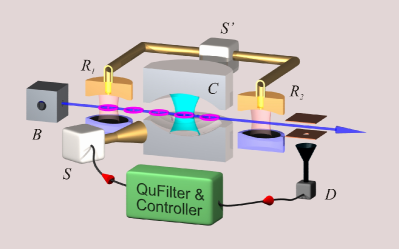
Figure 1: Proposed quantum feedback scheme adapted to a microwave cavity QED set-up. $C$: high-$Q$ microwave cavity, $B$: box producing Rydberg atoms, $R_{1}$ and $R_{2}$: low-$Q$ Ramsey cavities, $D$: atomic field-ionization detector, $S$ and $S^{\prime}$: microwave sources coupled to $C$ and $R$’s, respectively. In a quantum filtering process, a real-time control system analyzes the results of QND measurements of the cavity field and computes the amplitude of a control injection pulse.

Our quantum feedback algorithm is designed for the ENS microwave cavity QED set-up Raimond01 ; Deleglise08 . Its components are depicted in Fig. 1. The microwave field to be controlled is confined in an ultra-high $Q$ superconducting cavity $C$ (damping time $T_{\text{cav}}=0.13$ s). Rydberg atoms, flying one by one at 250 m/s across the cavity mode and dispersively interacting with its field, are used as QND probes of light Guerlin07 . They are prepared in a superposition of two circular Rydberg states $\left|e\right>$ and $\left|g\right>$ (principal quantum numbers 51 and 50, respectively) in the low-$Q$ cavity $R_{1}$, driven by the source $S^{\prime}$, in which they experience a resonant $\pi/2$-pulse. In the Bloch sphere representation, the spin corresponding to the two-level atomic system then points along the $Ox$ direction in the equatorial plane (states $\left|e\right>$ and $\left|g\right>$ correspond to north and south poles of the sphere, respectively; we use a frame rotating at the atomic frequency).

The light shifts experienced by the non-resonant $\left|g\right>\rightarrow\left|e\right>$ atomic transition in the cavity field result in a phase shift for the atomic state superposition. At the cavity exit, the atomic spin points along a direction in the equatorial plane at an angle $\Phi(n)$ with the $Ox$ axis, correlated to the photon number $n$. The dephasing angle $\Phi(n)$ can be controlled by adjusting the atom-cavity detuning $\delta$ and the interaction time. In the large atom-cavity detuning regime, it is a linear function of $n$: $\Phi(n)\sim(\Omega_{0}^{2}/4\delta)n$, where $\Omega_{0}/2\pi=49$ kHz is the vacuum Rabi frequency. For the intermediate detuning values used in the experiments, it is a more complex, albeit perfectly known growing function of $n$. A second $\pi/2$ Ramsey pulse in $R_{2}$ (phase $\phi_{\text{R}}$ with respect to that of the pulse in $R_{1}$) followed by the atomic detection (in the $\{\left|e\right>,\left|g\right>\}$ basis) by the detector $D$ amounts to a detection of the atomic spin along an axis at an angle $\phi_{\text{R}}$ with $Ox$. It provides information on the cavity field intensity.

Atoms are sent in the set-up at typical 250 $\mu$s time interval, much shorter than the cavity damping time. Note that such a macroscopic time interval is well adapted to elaborate feedback strategies since we have ample time to compute the state estimator and the feedback law between two atomic detections. When no feedback action is performed, the information provided by a few tens of atoms results in a measurement of the dephasing angle $\Phi(n)$ and, hence, in a projective QND measurement of the photon number $n$ Guerlin07 ; Brune08 .

We are interested here instead in the ambiguous information provided by a single atomic detection. Detection of the atomic state in $D$ projects the field, described initially by the density matrix $\rho_{\mathrm{}}$, onto a new state $\rho_{\mathrm{proj}}$. Depending on the detected atomic state, $\left|s\right>=\left|e\right>$ or $\left|g\right>$, the back-action of the quantum measurement on the field is described by

$$\rho_{\mathrm{proj}}=\frac{M_{s}\,\rho_{\mathrm{}}\,M_{s}^{\dagger}}{\text{Tr}\left(M_{s}\,\rho_{\mathrm{}}\,M_{s}^{\dagger}\right)},$$ (1)

where the operators $M_{s}$ are given by

$$M_{g}=\cos\left(\frac{\phi_{\text{R}}+\Phi({N})}{2}\right),$$ (2a)

$$M_{e}=\sin\left(\frac{\phi_{\text{R}}+\Phi({N})}{2}\right).$$ (2b)

Here, ${N}=a^{\dagger}a$ is the photon number operator with $a$ and $a^{\dagger}$ the photon annihilation and creation operators, respectively. The measurement operators $M_{s}$ are diagonal in a photon-number basis (as is $N$). They thus preserve Fock states, illustrating the QND nature of the measurement. The projected state (1) is normalized by the probability $P_{s}=\text{Tr}\left(M_{s}\rho M_{s}^{\dagger}\right)$ of detecting the atom in state $\left|s\right>$.

The cavity field can also be manipulated by injecting into the mode a coherent field pulse generated by the resonant microwave source $S$. Its action is described by the displacement operator $D(\alpha)=\exp(\alpha a^{\dagger}-\alpha^{*}a)$, where $\alpha$ is the complex amplitude of the injected field. The cavity field after displacement thus reads

$$\rho_{\mathrm{disp}}=D(\alpha)\,\rho\,D(-\alpha).$$ (3)

A proper analysis of the feedback scheme requires to take into account all known imperfections of the experimental set-up. Besides projective measurement (1) and coherent evolution (3), the cavity state also evolves due to decoherence. The field is coupled to a reservoir at non-zero temperature ($T=0.8$ K), and its dynamics is described by the master equation Walls94

$$\frac{d\rho}{dt}=\textbf{L}\rho\equiv-\frac{\kappa}{2}(1+n_{\text{th}})(a^{\dagger}a\rho+\rho aa^{\dagger}-2a\rho a^{\dagger})\\ -\frac{\kappa}{2}n_{\text{th}}(aa^{\dagger}\rho+\rho a^{\dagger}a-2a^{\dagger}\rho a),$$ (4)

where $\kappa=1/T_{\text{cav}}$ is the cavity decay rate and $n_{\text{th}}=0.05$ the equilibrium thermal photon number.

Moreover, the circular Rydberg state preparation is a non-deterministic Poisson process. We perform a pulsed excitation from a continuous thermal beam of Rubidium atoms, preparing atomic samples at a $T_{\text{a}}=85\,\mu$s time interval. The mean number of circular atoms per sample is $\eta_{\text{a}}\approx 0.3$ (leading to an average time between atoms of 250 $\mu$s). The atomic time of flight between $C$ and $D$ is 350 $\mu$s, corresponding to a delay of $d\!=\!4$ atomic samples. The probability for detecting an atom present in a sample is $\eta_{\text{d}}\approx 0.8$ due to finite detection efficiency in $D$. Finally, non-ideal atomic state resolution of the field-ionization detector and finite contrast of the Ramsey interferometer introduce a probability of erroneous state assignation of $\eta_{\text{f}}\approx 0.1$.

III Idealized experiment

In order to describe the essential elements of the feedback scheme in a simple context, we first consider in this Section an idealized experiment with no cavity decay ($\kappa=0$), a deterministic atomic preparation ($\eta_{\text{a}}=1$), no detection delay ($d=0$), and a perfect atomic detection ($\eta_{\text{d}}=1$ and $\eta_{\text{f}}=0$).

III.1 Quantum filter

The quantum filtering procedure Belavkin92 ; Bouten07 provides us with an estimate of the field state by using all available information. Right after detection of atom number $k$ and before injection of the corresponding control, it includes the initial state of the field $\rho_{0}$, information obtained from all $k$ atoms detected so far (labelled $i=1\ldots k$) and all coherent field injections performed in the former feedback loops (1 to $k\!-\!1$). Each of the elementary processes (atomic detections and displacements) can be represented by super-operators acting on the field’s density matrix. Let us note $\mathbf{M_{\text{}}}_{i}$ that associated to the detection of atom $i$ and $\mathbf{D_{\text{}}}_{i}$ that corresponding to the displacement performed in the $i^{\mathrm{th}}$ iteration of the feedback loop. Therefore, after detecting atom $k$, the state of the field is

$$\rho_{k}=\mathbf{M_{\text{}}}_{k}\left(\prod_{i=1}^{k-1}\mathbf{D_{\text{}}}_{i}\mathbf{M_{\text{}}}_{i}\right)\,\rho_{0}.$$ (5)

Here and in the following, all super-operator products are ordered by decreasing indices. Note that the expression (5) can be computed iteratively from the recurrence

$$\rho_{k+1}=\mathbf{M_{\text{}}}_{k+1}\mathbf{D_{\text{}}}_{k}\rho_{k},$$ (6)

setting $\mathbf{D_{\text{}}}_{0}=\openone$. By applying this filter recursively at each cycle, we get a reliable real-time estimate of the field state.

Based on Eqs. (1) and (3), the super-operators are defined as

$$\mathbf{M_{\text{}}}_{i}\,\rho = \frac{M_{s_{i}}\rho M_{s_{i}}^{\dagger}}{\text{Tr}\left(M_{s_{i}}\rho M_{s_{i}}^{\dagger}\right)}\,,$$ (7)

$$\mathbf{D_{\text{}}}_{i}\,\rho = D(\alpha_{i})\,\rho\,D(-\alpha_{i})\,.$$ (8)

Here, $s_{i}=g$ or $e$ depending on the outcome of the $i^{\mathrm{th}}$ atomic measurement. The control amplitude $\alpha_{i}$ is adjusted after each atom detection according to the feedback law described in the next subsection.

We choose to prepare initially the cavity in a coherent state with a mean photon number equal to the target value $n_{\text{\tiny tag}}$. The phase of this field is used as a reference. As a consequence, its amplitude $\alpha_{0}=\sqrt{n}_{\text{\tiny tag}}$ is real. The phase $\phi_{\text{R}}$ and the operator $\Phi(N)$, defining the measurement super-operators $\mathbf{M_{\text{}}}_{i}$ through (2), should be adjusted to optimize the quantum filter (6). On the one hand, the mean dephasing angle per photon $\bar{\phi}$ (estimated in the useful range of $n$ values) should be large in order to resolve adjacent photon numbers. On the other hand, the measurement should lift the ambiguity between a large range of possible photon numbers from $0$ to some $n_{\text{\tiny max}}$, determined by the spread of the initial coherent field. Due to the oscillating nature of the measurement operators $M_{s}$, this sets a maximum value of $\bar{\phi}$ of the order of $\pi/n_{\text{\tiny max}}$.

Finally, we need to optimally distinguish $n_{\text{\tiny tag}}$ from $n_{\text{\tiny tag}}\pm 1$. This is achieved by setting the Ramsey phase $\phi_{\text{R}}$ so that $(\phi_{\text{R}}+\Phi(n_{\text{\tiny tag}}))/2=\pi/4$. This setting corresponds to a maximal variation of the atomic state detection probabilities around $n_{\text{\tiny tag}}$. In other words, we set the atomic Ramsey interferometer at mid-fringe when the cavity contains $n_{\text{\tiny tag}}$ photons.

III.2 Feedback control

The distance between $\rho_{k}$ and the target Fock state described by a density operator $\rho_{\text{\tiny tag}}=\left|n_{\text{\tiny tag}}\right>\left<n_{\text{\tiny tag}}\right|$ can be conveniently defined as

$$V(\rho_{k})=1-\text{Tr}\left(\rho_{k}\rho_{\text{\tiny tag}}\right)\equiv 1-F(\rho_{k}),$$ (9)

where $F(\rho)=\text{Tr}\left(\rho\,\rho_{\text{\tiny tag}}\right)$ is the fidelity of a state $\rho$ with respect to the target state $\rho_{\text{\tiny tag}}$. The function $V(\rho)$ represents a natural choice for the Lyapunov function Mirrahimi07 used to study the stability properties of the quantum controller. This study is presented in more detail in Ref. Mirrahimi09 .

Let us denote the cavity state after the control displacement in the $k^{\mathrm{th}}$ iteration of the feedback loop as $\tilde{\rho}_{k}=\mathbf{D_{\text{}}}_{k}\rho_{k}$. The optimal convergence of the feedback procedure is obtained by finding at each cycle the injection amplitude $\alpha_{k}$ which maximizes the fidelity $F(\tilde{\rho}_{k})$. This search can be performed in a straightforward way by numerical optimization. However, this approach is time-consuming and could not be realistically implemented with existing real-time data analysis systems in the few tens of microseconds time interval between two atomic detections. We overcome this difficulty by developing a faster, analytical calculation of a locally optimal displacement $\alpha_{k}$. Since the measurement operators, the initial density matrix and the projector on the target Fock state are all real operators, we can reasonably choose $\alpha_{k}$ to be real. The field density matrix then remains always real.

In the limit of small $\alpha$, the Baker-Campbell-Hausdorff formula Barnett03 yields the following approximation for a displaced state (3):

$$\tilde{\rho}=D(\alpha)\rho D(-\alpha)\approx\, \rho-\alpha[\rho,a^{\dagger}-a]$$

$$+\frac{\alpha^{2}}{2}[[\rho,a^{\dagger}-a],a^{\dagger}-a].$$ (10)

Using (8), we therefore get for small $\alpha_{k}$

$$F(\tilde{\rho}_{k})=F(\rho_{k})-\alpha_{k}\text{Tr}\left([\rho_{k},a^{\dagger}\!-\!a]\rho_{\text{\tiny tag}}\right)\\ +\frac{\alpha_{k}^{2}}{2}\text{Tr}\left([[\rho_{k},a^{\dagger}\!-\!a],a^{\dagger}\!-\!a]\rho_{\text{\tiny tag}}\right)\,.$$ (11)

Choosing the feedback amplitude as

$$\alpha_{k}=-c_{1}\text{Tr}\left([\rho_{k},a^{\dagger}\!-\!a]\rho_{\text{\tiny tag}}\right),$$ (12)

with a gain $c_{1}>0$ small enough ensures that

$$F(\tilde{\rho}_{k})>F(\rho_{k})$$ (13)

as soon as the trace in (12) is strictly positive. Furthermore, since $[\rho_{\text{\tiny tag}},M_{g}]=[\rho_{\text{\tiny tag}},M_{e}]=0$ and $M_{g}^{\dagger}M_{g}+M_{e}^{\dagger}M_{e}=\openone$, the conditional expectation of $F(\rho_{k+1})$ knowing $\tilde{\rho}_{k}$ is given by

$${\text{\large$\mathbb{E}$}}\left(F(\rho_{k+1})\leavevmode\nobreak\ |\leavevmode\nobreak\ \tilde{\rho}_{k}\right)=P_{g,k}\text{Tr}\left(\frac{\rho_{\text{\tiny tag}}M_{g}\tilde{\rho}_{k}M_{g}^{\dagger}}{P_{g,k}}\right)\\ +P_{e,k}\text{Tr}\left(\frac{\rho_{\text{\tiny tag}}M_{e}\tilde{\rho}_{k}M_{e}^{\dagger}}{P_{e,k}}\right)=F(\tilde{\rho}_{k}).$$ (14)

Therefore

$${\text{\large$\mathbb{E}$}}\left(F\big{(}\tilde{\rho}_{k+1}\big{)}\leavevmode\nobreak\ |\leavevmode\nobreak\ \tilde{\rho}_{k}\right)\geq{\text{\large$\mathbb{E}$}}\left(F\big{(}\rho_{k+1}\big{)}\leavevmode\nobreak\ |\leavevmode\nobreak\ \tilde{\rho}_{k}\right)=F(\tilde{\rho}_{k})$$ (15)

and, as a result, the expectation value of $F(\tilde{\rho}_{k})$ is a non-decreasing function of $k$:

$$1\geq{\text{\large$\mathbb{E}$}}\left(F\big{(}\tilde{\rho}_{k+1}\big{)}\right)\geq{\text{\large$\mathbb{E}$}}\left(F\big{(}\tilde{\rho}_{k}\big{)}\right)\geq 0.$$ (16)

We have only shown so far that $F(\tilde{\rho}_{k})$ is increasing on the average. It does not mean that, for all individual realizations of the loop sequence, $F(\tilde{\rho}_{k})$ converges to 1, its maximum value reached when $\rho$ is equal to $\rho_{\text{\tiny tag}}$. Indeed, the feedback law (12) does not prevent the convergence towards other Fock states, since $\alpha_{k}=0$ whenever $\rho_{k}$ is the projector on any photon number state. A careful analysis shows that, in each realization, $F(\tilde{\rho}_{k})$ converges either to 1 or, with some small probability, to zero. To overcome this spurious attraction towards wrong photon number states, we propose, as in Mirrahimi07 , to modify the feedback law (12) by applying a constant injection “kick” as soon as the cavity state significantly deviates from the target:

$$\alpha_{k}\!=\!\left\{\!\begin{array}[]{ll}c_{1}\text{Tr}\left([\rho_{\text{\tiny tag}}\,,a^{\dagger}\!-\!a]\rho_{k}\right)&\mbox{ if }F(\rho_{k})\geq\varepsilon,\\ \\ c_{2}\,\text{sign}\left(n_{\text{\tiny tag}}\!-n_{k}\right)&\mbox{ if }F(\rho_{k})<\varepsilon.\\ \end{array}\right.$$ (17)

Here, $n_{k}$ is the mean photon number in the current state $\rho_{k}$, $c_{2}>0$ is a constant kick amplitude. The kick condition is set by $\varepsilon$ with $1\!\gg\!\varepsilon\!>\!0$. In this way, by breaking attraction towards other Fock states, we make sure that the cavity state converges towards the target one.

The controller gain $c_{1}$ in (17) must be tuned to maximize fidelity $F(\tilde{\rho}_{k})$ at each sampling time $k$. Up to third-order terms in $(\rho_{k}\!-\rho_{\text{\tiny tag}})$, Eq. (11) yields

$$F(\tilde{\rho}_{k})=F(\rho_{k})\,+\\ \Big{(}\text{Tr}\left([\rho_{\text{\tiny tag}},a^{\dagger}\!-\!a]\rho_{k}\right)\!\Big{)}^{2}\left(c_{1}\!-\!\frac{c_{1}^{2}}{2}\text{Tr}\left([\rho_{\text{\tiny tag}},a^{\dagger}\!-\!a]^{2}\right)\!\right)\!.$$ (18)

By maximizing this expression, we find that the gain

$$c_{1}=\text{Tr}\left([\rho_{\text{\tiny tag}},a^{\dagger}\!-\!a]^{2}\right)^{-1}\!=(4n_{\text{\tiny tag}}\!+2)^{-1}$$ (19)

provides the fastest convergence speed in the vicinity of $\rho_{\text{\tiny tag}}$. A detailed mathematical analysis and a convergence proof of this feedback-scheme will be given in Mirrahimi09 .

III.3 Simulations

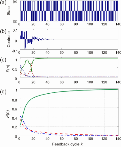
Figure 2: A single closed-loop quantum trajectory of an ideal measurement with $|n_{\text{\tiny tag}}\rangle=|3\rangle$. (a) Atomic states detected at each feedback cycle. (b) Control injections $\alpha_{k}$. (c) Evolution of photon number probabilities $P(n\!<\!n_{\text{\tiny tag}})$, $P(n_{\text{\tiny tag}})$ and $P(n\!>\!n_{\text{\tiny tag}})$ shown as dashed-dot blue, solid green and dashed red curve, respectively. (d) Average over $10^{4}$ closed-loop quantum trajectories.

To assess the performance of the proposed feedback scheme, we have performed quantum Monte-Carlo numerical simulations. Figure 2(a)-(c) presents a single quantum closed-loop trajectory in the ideal measurement setting, with a target Fock state $|n_{\text{\tiny tag}}\rangle=|3\rangle$. The Hilbert space is limited to $n_{\text{\tiny max}}=9$ photons. The atom-cavity detuning is set to $\delta/2\pi=238$ kHz. The mean dephasing angle per photon around $n_{\text{\tiny tag}}$ is then about $\pi/7$. Intuitively, the Ramsey phase $\phi_{\text{R}}$ should be set at the mid-fringe setting for $n_{\text{\tiny tag}}$ photons, i.e., $(\phi_{\text{R},0}+\Phi(n_{\text{\tiny tag}}))/2=\pi/4$. We have numerically observed that the convergence of the process is faster when the Ramsey phase alternates between four values in successive feedback cycles: $\phi_{\text{R},0}$, $(\phi_{\text{R},0}+\sigma_{\text{R}})$, $\phi_{\text{R},0}$ and $(\phi_{\text{R},0}-\sigma_{\text{R}})$. The phase excursion $\sigma_{\text{R}}$ is set at $0.69$ rad. The kick amplitude $c_{2}$ is 0.1 with a kick zone defined by $\varepsilon=0.1$. The initial cavity field $\rho_{0}$ is the coherent state with 3 photons on the average, $\rho_{0}=D\left(\sqrt{3}\right)\left|0\right>\left<0\right|D\left(-\sqrt{3}\right)$.

The upper trace in Fig. 2 shows a sequence of detected atomic state. The corresponding control inputs $\alpha_{k}$ are plotted in the next panel. Large at the beginning, $\alpha_{k}$ rapidly converges towards zero. Figure 2(c) shows the probability for the number of photons in the cavity field to be smaller, equal or larger than $n_{\text{\tiny tag}}$ (dashed-dot blue, solid green and dashed red curve, respectively). For this particular quantum trajectory, we observe that $\rho$ converges to $\rho_{\text{\tiny tag}}$ in less than $30$ feedback cycles.

Figure 2(d) presents an ensemble average over $10^{4}$ realizations of the same numerical feedback experiment. The fidelity $F(\tilde{\rho}_{k})$ reaches values above $0.99$ after $140$ cycles. After 20 cycles only, about $80\%$ of the trajectories have converged to the target state, illustrating the efficiency of the feedback method.

IV Realistic experiment

So far, we have neglected experimental imperfections. In this Section, we take into account all known imperfections of the present experimental set-up: finite cavity lifetime, Poisson distribution of the atom number in atomic samples, non-ideal efficiency and state-selectivity of the detector and, finally, the finite delay between atom-cavity interaction and atomic detection. Below, we introduce modifications of the quantum filter (6), which make the process efficient in spite of these imperfections.

IV.1 Modified quantum filter

The quantum filtering process must provide us with a density matrix describing all our knowledge of the cavity field at a given time. We chose here this time to be right before the injection of the actuator pulse in the $k^{\mathrm{th}}$ iteration of the loop, after detection of the $k^{\mathrm{th}}$ atom. At this time, our knowledge includes all atomic measurements so far (from 1 to $k$), all displacements performed and the known relaxation of the cavity field in between these events. It must also include the influence of the $d$ atomic samples which have interacted with the cavity, but are still flying towards the detector when we record atomic sample $k$. All this information can, as above, be represented by super-operators acting on the field’s density matrix.

Let us note $\mathbf{P_{\text{}}}_{s}$ the super-operator describing the detection of an atomic sample. Each detection has three possible outcomes, labelled $s=e$, $g$ or $u$ (atom detected in $e$, $g$ or no detected atom at all). The super-operator $\mathbf{N_{\text{}}}$ describes the action of one of the $d$ atomic samples flying from $C$ to $D$. The displacement super-operator $\mathbf{D_{\text{}}}$ is given by (3) and the field relaxation during the time interval between atomic samples is described by $\mathbf{T_{\text{}}}$. The exact expressions of all these super-operators will be given later.

Therefore, the state of the cavity field before injection is

$$\rho_{k}=\mathbf{F}_{\text{2},k}\,\mathbf{F}_{\text{1},k}\,\rho_{0},$$ (20)

where

$$\mathbf{F}_{\text{1},k}=\mathbf{T_{\text{}}}\mathbf{P_{\text{}}}_{s_{k}}\prod_{i=1}^{k-1}\mathbf{D_{\text{}}}_{i-d}\mathbf{T_{\text{}}}\mathbf{P_{\text{}}}_{s_{i}}$$ (21)

includes the information gathered by the first $k$ sample detections and

$$\mathbf{F}_{\text{2},k}=\prod_{i=k}^{k+d-1}\mathbf{T_{\text{}}}\mathbf{N_{\text{}}}\mathbf{D_{\text{}}}_{i-d}$$ (22)

includes the influence of the $d$ in-flight samples. Note that due to the atomic propagation delay between $C$ and $D$, the displacement amplitude injected in $C$ right after atomic sample $i$ has interacted with it is $\alpha_{i-d}$, computed in the $(i-d)$-th iteration of the loop. Hence, the first $d$ atomic samples cross the cavity before any displacement. This is formally taken into account by setting $\mathbf{D_{\text{}}}_{i}$ to unity for non-positive indices. If $d=0$, i.e. for no delay in the detection process, the empty product in (22) equals by convention the identity operator. Consequently, in the case of the ideal experimental parameters, the expression (20) naturally reduces to (5).

The density operator $\rho_{k}$ is used in the feedback law (17) to calculate the control injection $\alpha_{k}$. The product $\mathbf{F}_{\text{1},k}$ can be easily computed recursively, as in the ideal case. However, we must recalculate $\mathbf{F}_{\text{2},k}$ at each feedback cycle.

We now give the explicit expression of all super-operators considered so far. The measurement process $\mathbf{P_{\text{}}}_{s}$ takes into account detector’s imperfections and non-ideal atomic source. If the detector clicks and indicates state $|s\rangle=|g\rangle$ or $|e\rangle$, the new quantum state is a statistical weighted mixture of two projected states. The strongest weight corresponds to the projection according to the recorded outcome. With a smaller probability, the atomic detection has been erroneous. The atom was, at detection time, in the state $\left|\overline{s}\right>$, opposite to $\left|s\right>$, and the field has been projected accordingly. Thus, due to the imperfections of state discrimination alone, we get

$$\mathbf{P_{\text{}}}_{(s=e/g)}\,\rho=(1-P_{\text{f}})\mathbf{M_{\text{}}}_{s}\rho+P_{\text{f}}\mathbf{M_{\text{}}}_{\overline{s}}\rho\,.$$ (23)

The weights of the two projected states are given by the conditional probability of a wrong detection knowing that the detector has clicked in $|s\rangle$: $P_{\text{f}}=\eta_{\text{f}}P_{\overline{s}}/\left((1-\eta_{\text{f}})P_{s}+\eta_{\text{f}}P_{\overline{s}}\right)$ with $P_{s}=\text{Tr}\left(M_{s}\rho M_{s}^{\dagger}\right)$.

If the detector does not click (outcome $s=u$), either there was no atom in the sample or an atom was present but has not been detected. Therefore, the estimated state is a mixture of the unperturbed cavity field and of the two projected states corresponding to the two possible states of the undetected atom (we assume here that these two states are equiprobable). We thus get

$$\mathbf{P_{\text{}}}_{(s=u)}\,\rho=(1\!-\!P_{u})\rho+P_{u}\left(M_{g}\rho M_{g}^{\dagger}\!+\!M_{e}\rho M_{e}^{\dagger}\right).$$ (24)

The weights in this mixture are set by the conditional probability to have an undetected atom in a sample: $P_{u}=\eta_{\text{a}}(1-\eta_{\text{d}})/(1-\eta_{\text{a}}\eta_{\text{d}})$.

The interaction with a not-yet-detected sample is described by the super-operator $\mathbf{N_{\text{}}}$. It is given by (24) with the conditional probability $P_{u}$ replaced by the atomic sample occupation probability $\eta_{\text{a}}$, since the measurement has not been performed yet, resulting in

$$\mathbf{N_{\text{}}}\rho=(1\!-\!\eta_{\text{a}})\rho+\eta_{\text{a}}\left(M_{g}\rho M_{g}^{\dagger}\!+\!M_{e}\rho M_{e}^{\dagger}\right).$$ (25)

The super-operator $\mathbf{T_{\text{}}}$ describes the evolution due to the cavity field relaxation during the time interval $T_{\text{a}}$ between two atomic samples. Using (4) in the approximation of small time interval, $T_{\text{a}}\!\ll\!T_{\text{cav}}$, we get

$$\mathbf{T_{\text{}}}\rho=(\openone+T_{\text{a}}\textbf{L})\rho\,.$$ (26)

IV.2 Simulations

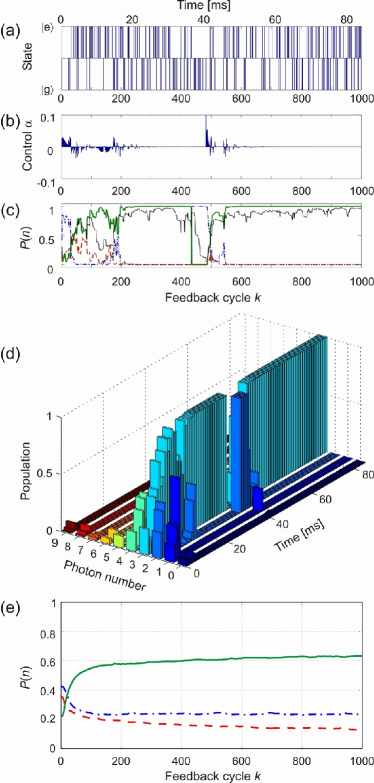
Figure 3: A single closed-loop quantum trajectory for realistic experimental parameters with $|n_{\text{\tiny tag}}\rangle=|3\rangle$. (a) Sequence of detected atomic states. (b) Control injections $\alpha_{k}$. (c) Evolution of the photon number probabilities $P(n\!<\!n_{\text{\tiny tag}})$, $P(n_{\text{\tiny tag}})$ and $P(n\!>\!n_{\text{\tiny tag}})$ (dashed-dot blue, solid green and dashed red curve, respectively) of the field state $\rho^{\text{\tiny real}}$ deduced from the Monte-Carlo simulation. The thin black line gives the estimated state fidelity $F(\rho_{k})$. (d) Photon number probabilities for $n=0$ to $9$ in $\rho^{\text{\tiny real}}$. For better clarity, results of only one out of each 10 feedback cycles are shown. (e) Average over $10^{4}$ closed-loop quantum trajectories. If the number of quantum trajectories is large enough (as is the case here), the averaged photon number probabilities calculated from the real field states $\rho^{\text{\tiny real}}$ coincide with those averaged over the estimated states.

We have performed extensive simulations, similar to those of the idealized measurement in Fig. 2, with the feedback algorithm adapted to the realistic experimental parameters, given in Sec. II. We use Monte-Carlo simulations to follow the state of the cavity along individual realizations of the experiment. The field relaxation is taken into account by simulating random quantum jumps, whose average effect is described by Eq. (26) Haroche06 . For each atomic sample, we choose randomly the number of atoms ($0$ or $1$) and the real atomic state ($\left|e\right>$ or $\left|g\right>$) which would be detected by the ideal detector. These results determine uniquely the subsequent field state $\rho^{\text{\tiny real}}_{k}$. We then take into account the detection imperfections to simulate the outcomes of the realistic measurement, which are used in the feedback loop for computing $\rho_{k}$. Note that $\rho^{\text{\tiny real}}$ is not accessible in the experiment. Here, we use it to simulate the evolution of the field and, by comparing it with the state estimated in the quantum filtering process, to characterize the feedback performance. In the ideal case, considered in Sec. III, the estimated state $\rho_{k}$ always coincide with the real state of the field $\rho^{\text{\tiny real}}_{k}$.

Figure 3(a)-(d) shows a typical quantum trajectory, illustrating the robustness of our feedback scheme at the present level of imperfections. The first difference with the ideal case is the presence of many feedback cycles with no detected atoms. Nevertheless, after about $k\!=\!100$ feedback cycles (each of $85\,\mu$s duration), corresponding to approximatively $k\eta_{\text{a}}\!\approx\!30$ atoms and $k\eta_{\text{a}}\eta_{\text{d}}\!\approx\!24$ detector clicks, the cavity state successfully converges to the target Fock state  $|n_{\text{\tiny tag}}\rangle=|3\rangle$.

The other striking feature is the presence of sudden photon jumps due to the limited cavity lifetime. In this particular trajectory, a photon loss occurred at feedback cycle number $k\!\approx\!430$ (at about 37 ms). One sees that about 60 cycles (about 5 ms) are required to detect the jump before applying a large control displacement and about 60 more cycles to restore the target photon number in the cavity field.

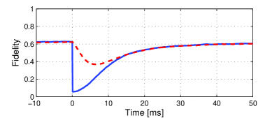
Figure 4: Feedback performance in the presence of a sudden photon number loss. The fidelity of the actual cavity state $\rho^{\text{\tiny real}}_{k}$ (blue solid curve) and of the state estimated by the quantum filtering process $\rho_{k}$ (red dashed curve) are defined with respect to the target Fock state and are obtained by averaging over $10^{4}$ quantum trajectories. In each trajectory, the time origin is shifted to the time of a quantum jump.

Figure 3(e) shows the same type of ensemble average as presented in Fig. 2(d). We observe a convergence towards a fidelity of $0.63$ after several hundred cycles resulting in about 100 detector clicks. This convergence, given as the number of actually detected atoms, is similar to that observed in the ideal case. The main difference between the two traces is the reduced asymptotic value of the fidelity of the prepared state: $F=0.63$ instead of $F=1$ in the ideal case. This reduction is mainly due to the cavity decay, which results in uncontrolled jumps of the photon number. The observed fidelity indicates that for a typical closed-loop trajectory the field stays in the state $|3\rangle$ about $63\,\%$ of time. Since the lifetime of $|n_{\text{\tiny tag}}\rangle$ is given by $T_{\text{cav}}/((1+n_{\text{th}})n_{\text{\tiny tag}}+n_{\text{th}}(n+1))=45$ ms Brune08 , we estimate that it takes on the average 26 ms to restore the initial Fock state after a sudden jump.

In order to observe in more detail the recovery of the system after a sudden photon jump, we recorded $10^{4}$ quantum trajectories showing sudden photon losses at different times. Before averaging the trajectories, we shift their individual time origins to the time of a jump. Figure 4 shows the evolution of the fidelity of the actual (solid curve) and estimated (dashed curve) cavity states with respect to $\rho_{\text{\tiny tag}}$. As calculated before, it takes about $20-30$ ms to restore the initial photon number state after a sudden photon loss.

The maximum fidelity of the quantum feedback, seen in Figs. 3-4 and corresponding to the ensemble of many realizations, shows how well a chosen photon number state can be preserved on average from its unavoidable decay. However, since in each feedback cycle we acquire actual information on the field, the fidelity of the deterministic generation of Fock states in a single realization can be much higher. To reliably produce the target state $\rho_{\text{\tiny tag}}$ we keep the feedback process running until we detect its successful convergence to $\rho_{\text{\tiny tag}}$ with an estimated fidelity better than $F_{\text{conv}}$. Figure 5(a) shows a histogram of convergence times for $F_{\text{conv}}=95\,\%$ obtained from $10^{4}$ quantum trajectories. The cumulative distribution, presented by a solid line, shows that after 20 ms the probability of a successful feedback outcome reaches $50\,\%$ and that it exceeds $90\,\%$ after 85 ms of the feedback operation. The inset in Fig. 5(a) shows the average density matrix of converged states with the population in $|n_{\text{\tiny tag}}\rangle$ of about $95\,\%$.

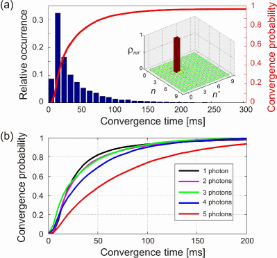
Figure 5: Feedback convergence. (a) Histogram of convergence times with $F_{\text{conv}}=0.95$. The solid line gives the probability of the feedback convergence after a given time. The inset shows the average density matrix of the converged states. (b) Convergence for several different Fock states. These curves result from an average over $10^{4}$ quantum trajectories.

Our feedback scheme can be tuned to generate any small photon number states. Figure 5(b) illustrates the convergence for several Fock states from $|n_{\text{\tiny tag}}\rangle=|1\rangle$ to $|5\rangle$. By increasing $n_{\text{\tiny tag}}$, the initial photon number distribution gets broader as the photon number lifetime gets shorter. Therefore, the feedback performance slowly degrades, resulting in the increased convergence time for the same required fidelity $F_{\text{conv}}$.

IV.3 Real-time computation

Implementation of this quantum feedback scheme into a real experiment requires fast real-time analysis of the measured data, faster than duration $T_{\text{a}}$ of one feedback cycle. We have tested a real-time processing system $\mathrm{ADwin}$ (Jäger Messtechnik) allowing for fast data acquisition and analysis in combination with complex experiment control. After careful optimization of all feedback computations, the execution of one typical feedback cycle of the proposed scheme requires about 4000 floating-point operations. Our preliminary tests have revealed that the ADwin system needs for this task about $30\,\mu\mathrm{s}<T_{\text{a}}=85\,\mu$s. We are now working on the integration of this control system into our cavity QED set-up.

V Conclusion

We have presented a quantum feedback protocol designed to deterministically generate small photon number states of a trapped microwave field. The reliable estimation of the cavity state at each feedback cycle allows us to follow in real time the quantum jumps of the photon number and then to efficiently compensate them, thus protecting Fock states against decoherence.

The two main components of the feedback algorithm are the quantum filter, which estimates the actual state of the field based on the outcomes of QND measurements, and the feedback law computing the amplitude of a correction microwave pulse whose injection into the cavity mode maximizes the field fidelity with respect to a desired Fock state. Quantum Monte-Carlo simulations of the QND measurements and the quantum feedback response demonstrate the high reliability of our closed-loop scheme even in the presence of realistic experimental imperfections. This scheme is also robust with respect to an imprecise knowledge of the initial state, since the repeated measurements of the state corrects initial wrong or incomplete information. Convergence and stability proofs of these feedback schemes will be given elsewhere. For a first set of mathematical results, see Ref. Mirrahimi09 .

The presented scheme can be extended to include the Ramsey phase $\phi_{\text{R}}$ and the spin dephasing $\Phi(N)$ as additional control parameters of the feedback loop. This should help to optimize the QND measurement according to our estimate of the actual field state and thus to acquire more information on its dynamics. These studies are under the way.

Acknowledgements Work supported partially by Agence Nationale de la Recherche (projet ANR-05-BLAN-0200-01 and projet Blanc CQUID 06-3-13957), Japan Science and Technology Agency (JST) and EU (IP project SCALA).

References

- (1) C. Guerlin et al., Nature 448, 889 (2007)
- (2) H. M. Wiseman and G. J. Milburn, Phys. Rev. A 49, 4110 (1994)
- (3) S. Deléglise et al., Nature 455, 510 (2008)
- (4) V. P. Belavkin, J. Multivariate Anal. 42, 171 (1992)
- (5) L. Bouten, R. Van Handel and M. James, SIAM J. Contr. Optim. 46, 2199 (2007)
- (6) M. Mirrahimi, R. Van Handel, SIAM J. Contr. Optim. 46, 445 (2007)
- (7) J. M. Geremia, Phys. Rev. Lett. 97, 073601 (2006)
- (8) M. Mirrahimi, I. Dotsenko and P. Rouchon, in preparation (quant-ph/0903.0996)
- (9) J.-M. Raimond, M. Brune, and S. Haroche, Rev. Mod. Phys. 73, 565 (2001)
- (10) M. Brune et al., Phys. Rev. Lett. 101, 240402 (2008)
- (11) D. F. Walls and G. J. Milburn, Quantum Optics, (Springer, Berlin, 1994).
- (12) S. M. Barnett and P. M. Radmore, Methods in Theoretical Quantum Optics, (Oxford University Press, 2003).
- (13) S. Haroche and J.-M. Raimond, Exploring the Quantum, (Oxford University Press, 2006).