The globular clusters-stellar haloes connection in early type galaxies

Abstract

This paper explores if, and to what an extent, the stellar populations of early type galaxies can be traced through the colour distribution of their globular cluster systems. The analysis, based on a galaxy sample from the Virgo ACS data, is an extension of a previous approach that has been successful in the cases of the giant ellipticals NGC 1399 and NGC 4486, and assumes that the two dominant GC populations form along diffuse stellar populations sharing the cluster chemical abundances and spatial distributions. The results show that a) Integrated galaxy colours can be matched to within the photometric uncertainties and are consistent with a narrow range of ages; b) The inferred mass to luminosity ratios and stellar masses are within the range of values available in the literature; c) Most globular cluster systems occupy a thick plane in the volume space defined by the cluster formation efficiency, total stellar mass and projected surface mass density. The formation efficiency parameter of the red clusters shows a dependency with projected stellar mass density that is absent for the blue globulars. In turn, the brightest galaxies appear clearly detached from that plane as a possible consequence of major past mergers; d) The stellar mass-metallicity relation is relatively shallow but shows a slope change at $M_{*}\approx 10^{10}M_{\odot}$. Galaxies with smaller stellar masses show predominantly unimodal globular cluster colour distributions. This result may indicate that less massive galaxies are not able to retain chemically enriched intestellar matter.

1 Introduction

Pioneering ideas about the role of globular clusters (GC) as tracers of the formation history of galaxies come from Eggen, Lynden Bell & Sandage (1962) or, with a different perspective, from Searle & Zinn (1978). The evolution of this subject during recent years has been reviewed in Brodie & Strader (2006). A key issue in that context is the connection between GC and the “diffuse” stellar populations of the galaxies they are associated with. Some reasons allow to infer that such a link might not be simple. However, several papers point out that massive early type galaxies seem to have highly synchronised ages. For example, La Barbera et al. (2008) reach that conclusion in their discussion of the properties of the Fundamental Plane for early type galaxies also indicating that the age variation per mass decade seems smaller than a few percent. This suggests that the eventual connection between field stars and GC may still be “read” since the effects of subsequent (younger) stellar populations in these galaxies may have not been important.

The theoretical side of the problem has received a number of contributions in an effort to better define its cosmological background (e.g. Beasley et al. 2002 or,more recently, Bekki et al. 2008). Differences and similarities between GC and the underlying stellar populations have been pointed out in the past. For example, Forte, Strom and Strom (1981) found that, in the average, GC appear significantly bluer than the stellar halos at all galactocentric radii in four Virgo ellipticals.

In turn, and after the discovery of GC colour bimodality (e.g. Zepf & Ashman 1993; Ostrov, Geisler & Forte 1993) Forbes & Forte (2001) noted that the stellar halo colours in the inner regions of early type galaxies are remarkably similar to those of the “red” GC population.

A more recent comparison between the integrated features of the NGC 3923 galaxy halo and its GC population has been presented in Norris et al. (2008) on the basis of Gemini-GMOS spectra and direct imaging data. These authors show that the galaxy halo has a chemical abundance close to the average value defined by its GC and that both systems are coeval.

A point to be considered in that kind of comparisons, however, is that the GC colour statistics are “number weighted” while halo colours are, naturally, “luminosity” weighted. Thus, a coincidence between GC and stellar halo colours would be expected only if each GC is formed along a given diffuse stellar mass on a constant luminosity basis.

An alternative approach has been presented in Forte, Faifer & Geisler (2005) and Forte, Faifer & Geisler (2007) (hereafter FFG07) in a comparative study of the giant ellipticals NGC 1399 and NGC 4486 (M87). The main assumption in these works is that GC are good tracers of the spatial distribution and chemical abundance spread of “diffuse” stellar populations, formed along with the clusters, and that the number of GC, $N$, per diffuse stellar mass unit $M_{*}$ with chemical abundance $Z$, is given by

$$dN(Z)/dM_{*}(Z)={\gamma}\exp({-{\delta[Z/H])}}\$$ (1)

which is a generalization of the Zepf & Ashman (1993) T parameter. In those galaxies, the results show that the number of GC per diffuse stellar mass increases when metallicity decreases.

$\gamma$ and $\delta$ are free parameters that, once the spatial distribution of the GC and their chemical abundance scales are determined, allow a fit of the galaxy surface brightness profiles over several tens of Kpc. These fits also provide a good approximation to the galactocentric colour gradients as well as of the difference between galaxy halo colours and GC mean colours. In turn, the inferred metallicities for field stars show a remarkable similarity with the observed ones in nearby resolved galaxies.

This paper aims at further testing the modeling described above, taking advantage of the largest and most homogeneous GC data set available so far in the literature: The Virgo Advanced Camera Survey (Côté et al. 2004 and subsequent papers). In particular, we refer to the galaxy photometry presented by Ferrarese et al. 2006; hereafter F2006) and to the GC systems study by Peng et al. 2006; hereafter P2006 ). Figure 1 shows the colour difference between stellar halo colours and mean GC colours for a galaxy sub-sample (see paragraph 5) from F2006 and P2006. This diagram is consistent with the results in Forte et al. (1981) mentioned above.

Figure 1: $(g-z)$ colour difference between galaxy halo colours (from Ferrarese et al. 2006) and the average GC colours in each galaxy (from Peng et al. 2006).

A thorough discussion about the characteristics of the GC formation efficiencies in terms of galaxy brightness, mass, and environment within the Virgo cluster has been recently presented by Peng et al. (2008). This work shows that both the number of GC per galaxy brightness or galaxy mass units have a non monotonic behaviour reaching a minimum for galaxies with stellar masses $\approx 5.10^{10}M_{\odot}$ .

That overall trend, in turn, is compatible with the results obtained by Rhode, Zepf & Santos (2005) and later by Spitler et al. (2008), in their discussion of galaxies more massive than that mass, and also with those by Miller & Lotz (2007) in the analysis of GC systems associated to less massive dwarf galaxies.

In this paper we address the same subject although with some differences in comparison with Peng et al. (2008), namely:

-GC colour histograms are decomposed in terms of “blue” and “red” clusters using the FFG07 approach instead of the non-parametric fits performed by P2006.

-Stellar mass to B luminosity ratios are derived on the basis of the FFG07 modeling and used to estimate stellar masses within a galactocentric radius of $\approx$ 150 arcsecs, the typical coverage of the Virgo ACS.

-Cluster formation is analyzed in the volume space defined by GC formation efficiency, galaxy stellar mass, and projected stellar mass densities, as well as in terms of chemical abundances.

2 Model assumptions (and caveats)

The GC-stellar haloes link given in FFG07 involves several assumptions, namely:

a) GC colour bimodality in fact reflects two different (“blue” and “red”) GC families which have distinct chemical abundance and spatial distributions. Several arguments support this assumption (see Kundu & Zepf 2007; Strader et al. 2007).

b) GC colour histograms are usually decomposed via two-Gaussian fits that involve five free parameters. Instead, FFG07 seek for a link betweeen chemical abundance $Z$ and integrated colour by means of an empirical colour-metallicity relation (see paragraph 3). Exploring different trial functions leads to $N(Z)\approx exp(Z-Zi)/Zs$, where $Zi$ is an initial chemical abundance, as the simplest approximation for the colour histogram decomposition. In this work, as in FFG07, we set $Zi=0.0035Z_{\odot}$. The histogram fit then requires three parameters: the chemical abundance scale lenghts $Zs(blue)$, $Zs(red)$ and the relative fraction of clusters belonging to each GC family.

The case of the blue GC deserves a particular comment in relation with the presence of the so called “blue tilt”, i.e., these clusters seem to become redder with increasing brightness in some galaxies. This effect produces a spread of the blue GC colours that FFG07 identify as a variation of $Zi$ with cluster mass in the case of NGC 4486.

We note that the existence of the tilt in NGC 4486, is a subject of debate in the literature, e.g., Strader et al. (2006); Mieske et al. (2006), FFG07, Kundu (2008), or Waters et al. (2008).

c) Blue and red GC families are assumed to be old and formed within a relatively narrow period of time. Arguments supporting this assumption can be found, for example, in Brodie & Strader (2006) (see their figure 7).

Alternatively, some intermediate age globular candidates have been reported, among the “red” globulars in other galaxies, by Forbes et al. (2001) (also see Pierce et al. 2006a, Pierce et al. 2006b; Hempel et al. 2007).

d) The ratio of the number of GC to diffuse stellar mass with the same $Z$, is assumed to follow the exponential relation given in paragraph 1. For typical values of $\bf\delta$, that ratio increases when chemical abundance decreases. This is a “phenomenological” assumption, that allows a good fit to the surface brightness and halo colour gradients in NGC 1399 and NGC 4486, and that we confront with the Virgo ACS data in this work.

A caveat in the whole approach concerns to the fact that GC statistics refer to clusters that have survived to a number of destructive events of dynamical origin (Charlton & Laguna 1995; Gnedin & Ostriker 1997), i.e., these GC might not reflect the original cluster populations. For example, both the blue and red GC show cores in their projected galactocentric surface densities (although with widely different spatial scales) that may be the result of that depletion process. These cores contrast with the peaked brightness profiles in the inner region of galaxies.

3 The colour metalicity calibration

An empirical $(C-T_{1})$ colour versus $[Fe/H]_{zw}$ metallicity relation (on the Zinn & West 1984 scale) was presented in FFG07:

$$(C-T_{1})=0.94+0.068~{}([Fe/H]_{zw}+3.5)^{2}$$ (2)

This relation was obtained by combining 100 GC in the MW and 98 in other three galaxies whose metallicities were derived from Lick indices. This relation is also adopted in this work after transforming the $(g-z)$ colours to $(C-T_{1})$ as discussed in paragraph 4. A comparison with SSP models by Maraston (2005) and Bruzual & Charlot (2003), for an age of 12 Gy, is shown in Figure 2.

Figure 2: Integrated $(g-z)$ colour versus chemical abundance from SSP models for an age of 12 Gy. Filled circles: Maraston (2005)); open circles: Bruzual & Charlot (2003). The continuous line is the empirical calibration given by FFG07, adopting $[Z/H]=[Fe/H]_{zw}+0.131$, and $(g-z)=(C-T_{1})-0.20$ (see text).

Considering the $(g-z)$ and $(B-I)$ colours in the Maraston (2005) models, that leads to:

$$(g-z)=1.00~{}(B-I)-0.68$$ (3)

and the empirical $(B-I)$ versus $(C-T_{1})$ colours relation for MW clusters given in FFG07:

$$(C-T_{1})=1.03~{}(B-I)-0.43$$ (4)

indicates that $(C-T_{1})$ and $(g-z)$ can be linked just by means of a zero point difference, a procedure that we describe and adopt in the following paragraphs.

4 Photometric scales

For the sake of homogeneity with FFG07, we first transform the $g$ magnitudes given by F2006 to $B$ magnitudes (Johnson system). The $B$ luminosities, in turn, will be used to estimate the galaxy masses though the $(M/L)_{B}$ ratios derived from fits to the GC colour histograms.

The Virgo ACS survey has a field coverage of 3.4 arcmin, which roughly means a galactocentric range of $\approx 150$ arcsecs. Galaxy $g$ magnitudes were then obtained within an elliptical contour, with a semimajor axis a= 150 arcsecs, and using the Sérsic best fit parameters given in F2006 (table 3). In turn, integrated $B$ magnitudes, within that galactocentric range, were obtained for 14 galaxies, fainter than $B$=11.0 mag, in common with Caon et al. (1990) yielding:

$$B=g(150)+0.28~{}(\pm 0.19/\sqrt{14})$$ (5)

a transformation that we adopt in what follows.

This connection between the $g(150)$ and $B$ magnitudes can be also compared with that derived from the relations given by Rodgers et al. (2006) (based on stellar photometry), and adopting a mean colour $(g-z)$=1.3 for the ACS galaxies, leading to $B=g(150)+0.44$. The differences between both zero points give an idea about the photometric uncertainties involved in this kind of analysis.

The FFG07 modelling delivers $(C-T_{1})$ colours that can be transformed to $(g-z)$ just by adopting a colour offset (as discussed in the previous paragraph). First we look for the link between the $(C-T_{1})$ and $(g-z)$ colour scales from FFG07 and P2006, respectively, and using the photometry of the well populated GC system of NGC 4486 (VCC 1316). Figure 3 shows the $(C-T_{1})$ colour histogram for GC within a galactocentric range of 120 to 360 arcsecs from FFG07. This diagram also shows the GC histogram given by P2006 for the inner regions of the same galaxy, and adopting a shift

$$(C-T_{1})-(g-z)~{}(P2006)=0.29$$ (6)

that agrees with a previous estimate in FFG07. Vertical lines in Figure 3 indicate that the position of the “blue” and “red” GC peaks are consistent in both statistics (using the same binning steps as in P2006) and no variation of these peaks seem detectable with galactocentric radius. The same feature holds further out in galactocentric radius as shown by Kundu & Zepf (2007). We note that the blue tail of the GC colour distribution is more populated in the outer field, suggesting a somewhat bluer lower boundary in colour. The significance of this effect is hard to asses since the outer region is more likely to be affected by field interlopers (for example, unresolved blue galaxies).

Figure 3: $(C-T_{1})$ colour histogram for the NGC 4486 globular cluster candidates with galactocentric distances from 120 to 360 arcsecs (thin line) using the data from FFG07. The thick line corresponds to clusters within 150 arcsecs from the galaxy center as given by Peng et al. 2006. The binning steps are those defined in this last work. Vertical lines show the positions of the “blue” and “red” peaks. $(g-z)$ was transformed to $(C-T_{1})$ by adding 0.29 mags.(see text).

A similar approach was adopted regarding the galaxy integrated colours. F2006 give $(g-z)$ = 1.60 for NGC 4486 while the integration of the $B$ profile from Caon et al. (1990), combined with the (B-R) colour gradient listed by Michard (2000), leads to $(B-R)$ = 1.53 within a galactocentric radius of 150 arcsecs. Given the GC colour relations in FFG07, this colour transforms to ($C-T_{1})$ = 1.77 and then:

$$(C-T_{1})-(g-z)~{}(F2006)=0.17$$ (7)

The zero point difference between the F2006 and P2006 colour scales is coherent with the results given by Janz & Lisker (2009) in their analysis of the (g-z) colour magnitude relation of early type galaxies.

5 GC Colour Histogram fits

P2006 present $(g-z)$ colour histograms for GC systems in 100 Virgo galaxies (their figure 2). Our analysis is restricted to galaxies with more than $\approx$ 15 GC and at least five colour bins (after removing background contamination). Smaller cluster populations, or lower definition colour histograms, prevent meaningful fits.

There are four galaxy fields (P2006 numbers: 43, 61, 79, 93) that, being close to galaxies with large CG populations, might be likely contaminated by their GC. In turn, galaxy number 39 is the only unimodal galaxy with a narrow red peak. This last GC system, and those in galaxies 27, 32, 33 and 65, could not be properly fit due to noisy histograms or high background contamination. As a result of the criteria mentioned above, and after rejecting these last objects, our sample finally comprises 63 galaxies listed in Table 1.

P2006 perform a non-parametric fit to the GC histogram which, as mentioned, is different from the approach presented in this paper. Here we adopt a Monte Carlo based approach that seeks the determination of the chemical abundance scales, $Zs(blue)$ and $Zs(red)$, as well as the fraction of clusters in each GC population from the GC colour histograms.

First, a “seed” globular is randomly generated with a given $Z$ (controlled by an initial $Zs$ parameter). This value is transformed to $[Fe/H]_{zw}$ and to $(g-z)$ colour, by means of our colour-metallicity relation. Interstellar colour excesses and gaussian observational errors (with a dispersion $\pm$ 0.05 in $(g-z)$) are added to each cluster. The resulting synthetic histograms are then compared with those given by P2006 using the same variable binning steps adopted by these authors.

The $Zs$ values, and the ratio of clusters belonging to the blue or red populations, are iterated until a “quality fit” $\chi^{2}$ parameter, as defined by Côté et al. (1998), is minimised.

Throughout this analysis we use an average E(B-V) = 0.028, from the colour excesses given by F2006 which, in turn, are based on the Schlegel et al. (1998) maps. This seems justified by the uncertainties of these maps although, as noted by Peng et al. (2008), some noise would be expected on the derived blue luminosities arising in dust eventualy associated with each galaxy.

The resulting $Zs$ scales, number of clusters assigned to each GC family and the quality of the fit indicator, are given in Table 1. Typical uncertainties connected with counting statistics range from 0.005 to 0.01 for $Zs(blue)$ and 0.05 to 0.15 for $Zs(red)$.

Table 1: Globular cluster colour histogram fit parameters for Virgo ACS galaxies. Col. [1]: Galaxy number from P2006; Col. [2]: VCC galaxy number from Binggeli, Sandage & Tammann 1985; Col. [3]: Number of blue GC; Col. [4]: Chemical abundance scale for the blue GC in $Z_{\odot}$ units; Col. [5]: Number of red GC; Col. [6]: Chemical abundance scale for the red GC in $Z_{\odot}$ units; Col. [7]: GC colour histogram quality fit parameter (as in Côté et al. 1998); Col. [8]: Fraction of stellar mass associated with the red GC; Col. [9]: Integrated apparent g magnitude (within a=150 arcsecs); Col. [10]: Integrated (g-z) galaxy colours from F2006; Col. [11]: Integrated (g-z) galaxy colours from model fit; Col. [12]: Stellar mass to luminosity (B band) ratio from model fit.

$N_{P2006}$	VCC	$N_{blue}$	$Zs(blue)$	$N_{red}$	$Zs(red)$	$\chi^{2}$	F	$g(150)$	$(g-z)$	$(g-z)_{m}$	$(M/L)_{B}$
(1)	(2)	(3)	(4)	(5)	(6)	(7)	(8)	(9)	(10)	(11)	(12)
1	1226	188	0.037	562	0.90	2.18	0.97	9.21	1.60	1.60	9.45
2	1316	388	0.034	1337	0.85	3.65	0.98	9.84	1.60	1.60	9.39
3	1978	217	0.037	573	1.00	0.00	0.97	9.82	1.62	1.61	9.61
4	881	122	0.024	228	0.30	1.71	0.94	10.12	1.57	1.41	6.92
5	798	152	0.037	354	0.45	0.40	0.95	10.00	1.38	1.48	7.81
6	763	186	0.035	309	0.35	2.65	0.92	9.16	1.56	1.42	7.14
7	731	204	0.030	681	0.45	0.69	0.97	9.95	1.53	1.49	7.94
8	1535	70	0.018	164	0.65	0.35	0.98	—–	—-	1.55	8.80
9	1903	59	0.034	236	0.45	0.00	0.97	10.42	1.63	1.49	7.96
10	1632	113	0.075	338	0.60	2.09	0.94	10.66	1.61	1.53	8.47
11	1231	72	0.028	168	0.40	1.68	0.96	10.71	1.53	1.46	7.58
12	2095	38	0.063	88	0.30	0.00	0.90	11.71	1.44	1.40	6.87
13	1154	54	0.025	126	0.30	0.78	0.95	10.89	1.54	1.41	6.97
14	1062	47	0.050	106	0.60	0.88	0.95	11.06	1.53	1.52	8.42
15	2092	16	0.022	64	0.35	0.42	0.98	11.13	1.50	1.45	7.43
16	369	51	0.031	119	0.45	0.00	0.96	12.22	1.57	1.48	7.84
17	759	68	0.031	92	0.40	0.72	0.92	11.34	1.54	1.44	7.37
18	1692	60	0.025	60	0.50	1.03	0.92	11.65	1.53	1.47	7.79
19	1030	50	0.022	116	0.45	0.38	0.97	—–	—-	1.48	7.9
20	2000	102	0.025	83	0.25	1.09	0.86	11.71	1.51	1.34	6.24
21	685	78	0.031	78	0.50	1.24	0.91	11.59	1.55	1.46	7.71
22	1664	26	0.025	104	0.35	1.01	0.97	11.63	1.54	1.45	7.42
23	654	24	0.031	16	0.50	0.90	0.87	11.98	1.45	1.44	7.44
24	944	40	0.031	40	0.45	1.26	0.90	11.81	1.48	1.45	7.47
25	1938	49	0.021	40	0.20	0.27	0.85	11.77	1.49	1.31	5.90
26	1279	55	0.020	75	0.25	0.86	0.92	11.96	1.46	1.37	6.50
28	355	24	0.018	26	0.50	0.27	0.94	12.08	1.52	1.48	7.93
29	1619	12	0.018	43	0.30	0.13	0.97	12.18	1.42	1.42	7.09
30	1883	30	0.031	45	0.25	0.63	0.90	11.76	1.32	1.36	6.45
31	1242	38	0.031	72	0.30	0.97	0.93	12.19	1.46	1.40	6.87
34	778	22	0.025	38	0.30	0.42	0.93	12.67	1.47	1.40	6.88
35	1321	22	0.037	22	0.35	0.09	0.87	12.28	1.33	1.40	6.88
36	828	35	0.017	35	0.25	0.19	0.91	12.71	1.48	1.36	6.42
37	1250	22	0.025	22	0.08	0.55	0.75	12.40	1.21	1.19	4.79
38	1630	10	0.030	24	0.50	1.14	0.96	12.54	1.50	1.50	8.09
40	1025	65	0.044	35	0.30	0.00	0.74	12.61	1.43	1.33	6.17
41	1303	41	0.024	14	0.50	0.63	0.80	12.68	1.42	1.39	6.94
42	1913	22	0.031	33	0.60	0.38	0.94	12.90	1.43	1.51	8.35
44	1125	32	0.016	18	0.20	0.55	0.83	12.85	1.42	1.29	5.78
45	1475	38	0.031	38	0.15	1.31	0.80	13.06	1.35	1.27	5.49
46	1178	32	0.015	48	0.30	0.86	0.95	13.06	1.47	1.41	6.95
47	1283	29	0.022	26	0.30	0.47	0.89	13.02	1.47	1.38	6.66
48	1261	40	0.088	0	—–	0.46	0.00	13.29	1.20	1.22	4.96
49	698	25	0.015	85	0.10	—-	0.95	13.04	1.38	1.25	5.27
50	1422	25	0.101	0	—–	0.29	0.00	13.60	1.27	1.24	5.11
53	9	25	0.044	0	—–	0.73	0.00	13.81	1.15	1.14	4.36
57	856	35	0.056	0	—–	0.49	0.00	14.25	1.22	1.17	4.54
60	1087	45	0.044	0	—–	0.63	0.00	13.87	1.29	1.14	4.36
62	1861	35	0.094	0	—–	1.05	0.00	14.22	1.33	1.23	5.04
63	1431	65	0.075	0	0.05	0.60	0.00	14.12	1.24	1.20	4.80
63	543	20	0.031	0	—–	0.50	0.00	14.12	1.24	1.10	4.15
67	1833	20	0.101	0	—–	0.53	0.00	14.46	1.21	1.24	5.11
68	437	25	0.018	0	—–	0.91	0.00	13.82	1.26	1.05	3.93
71	200	15	0.018	0	—–	0.87	0.00	14.79	1.21	1.05	3.93
73	21	15	0.018	0	—–	0.74	0.00	14.79	0.82	1.05	3.93
78	1545	30	0.017	20	0.15	0.76	0.82	14.77	1.34	1.26	5.43
81	1075	20	0.025	0	—–	0.65	0.00	14.96	1.20	1.08	4.04
84	1440	21	0.018	9	0.50	0.00	0.87	14.67	1.26	1.42	7.33

Table 2: Table 1 – Continued.

$N_{P2006}$	VCC	$N_{blue}$	$Zs(blue)$	$N_{red}$	$Zs(red)$	$\chi^{2}$	F	$g(150)$	$(g-z)$	$(g-z)_{m}$	$(M/L)_{B}$
(1)	(2)	(3)	(4)	(5)	(6)	(7)	(8)	(9)	(10)	(11)	(12)
85	230	20	0.018	0	—–	0.92	0.00	15.45	1.17	1.05	3.93
89	1828	20	0.031	0	—–	0.50	0.00	15.09	1.25	1.10	4.15
91	1407	45	0.101	0	—–	0.60	0.00	15.03	1.23	1.24	5.11
95	1539	35	0.063	0	—–	0.00	0.00	15.15	1.21	1.18	4.63
96	1185	25	0.018	0	—–	0.66	0.00	15.24	1.28	1.05	3.93

A sample of histogram fits are shown in Figure 4 for some representative galaxies with different numbers of GC (upper row: galaxies with more than 250 GC; middle row: with 50 to 100 GC; lower row: with less than 50 GC). In this figure the fits are smoothed histograms adopting a Gaussian colour kernel of 0.03 mags on the model GC colours. In turn, the histogram fits for the 63 galaxies listed in Table 1, including the associated statistical counting uncertainties for each colour bin are displayed in the Appendix.

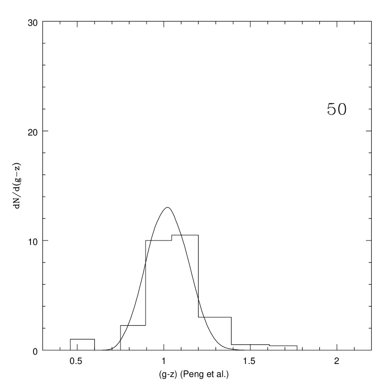
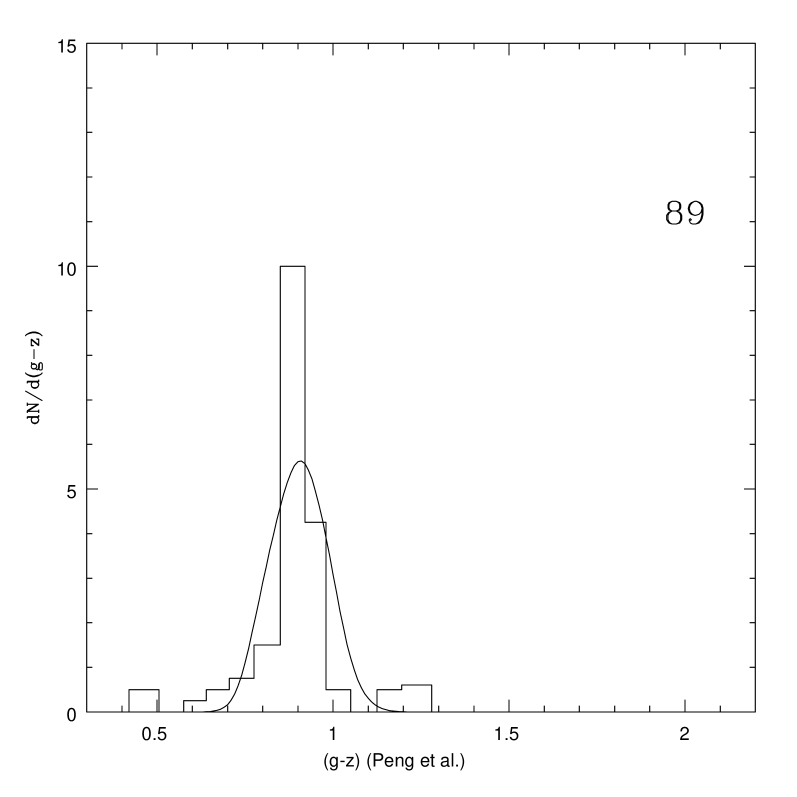
Figure 4: Sample GC colour histogram fits. Upper row: VCC 1226, VCC1978, VCC 798; middle row VCC 1938, VCC 1303, VCC 1283;lower row: VCC 1422, VCC 1828, VCC 1407. Upper right numbers are the galaxy identifications in Peng et al. (2006).

Figure 4 shows the same trend noted already by P2006. in the sense that GC colour bi-modality is clearly present in the brightest galaxies and becomes less evident, or is directly absent, in the faintest ones.

6 The $\gamma$ and $\delta$ parameters

This paragraph revises the values of the $\gamma$ and $\delta$ parameters given in FFG07 on the basis of the following arguments:

a) Those authors used $[Z/H]$ instead of $[Fe/H]_{zw}$ (as stated in the paper) as the argument of the adopted colour-metallicity relation used to obtain integrated model colours. That mistake is corrected in this work. As in FFG07, $[Z/H]$ is on the Thomas et al. (2004) chemical abundance scale and connected with $[Fe/H]_{zw}$ through $[Z/H]=[Fe/H]_{zw}+0.131$ as derived by Mendel, Proctor & Forbes (2007).

b) The $\bf\delta$ parameter was determined in FFG07 only trough the fit to the observed brightness profiles of NGC 1399 and NGC 4486. However, that parameter also controls the resulting galactocentric colour gradient. In this paper, we attempted a simultaneous fit to both the brightness and colour gradients, as given in Michard (2000) for these galaxies, aiming at minimizing the orthogonal sum of the rms of the brightness and colour fits.

c) $\bf\gamma$ and $\bf\delta$ were also derived for NGC 1427 using data from Forte et al. (2001). This galaxy was observed adopting the $(C-T_{1})$ index and using the same reduction and calibration procedures reported by FFG07.

The revised parameters for the three galaxies are listed in Table 3. In particular, the $\bf\delta$ parameters seem comparable (within the uncertainties) then suggesting that a similar pattern connects GC and stellar haloes in the three systems. We note that the average value, $\bf\delta$ = 1.75 that we adopt hereafter, is higher than those given in FFG07 ($\bf\delta$ = 1.10 and 1.20 ) for NGC 1399 and NGC 4486, respectively, after correcting the mistake noted in the first item of this paragraph.

Table 3: $\gamma$ and $\delta$ parameters for NGC 1399, NGC 1427 and NGC 4486.

	NGC 1399	NGC1427	NGC 4486
$\gamma~{}$ ($10^{-8}$ units)	0.73 $\pm$ 0.05	0.65 $\pm$ 0.03	0.75 $\pm$ 0.03
$\delta$	1.60 $\pm$ 0.15	1.90 $\pm$ 0.15	1.75 $\pm$ 0.10

7 Integrated colours, stellar mass-to-light ratios and galaxy masses

The model assumptions, i.e.:

$$dN/dZ=(N/Zs)\exp(-Z/Zs)\$$ (8)

where N is the number of globular clusters in the blue or red families and $Zs$ their respective abundance scales, and:

$$dN/dM_{*}(Z)={\gamma}\exp({-{\delta~{}[Z/H])}}\$$ (9)

imply that the amount of diffuse stellar mass with chemical abundance $Z$ will be given by:

$$M_{*}(Z)=\gamma^{-1}\exp(\delta~{}[Z/H])\big{[}\frac{N_{blue}}{Zs(blue)}\exp(-Z/Zs(blue))+$$

$$\frac{N_{red}}{Zs(red)}\exp(-Z/Zs(red))\big{]}$$ (10)

Both $N_{blue}$ and $N_{red}$ have distinct behaviours as a function of galactocentric radius which can be used to derive surface brightness profiles as shown in FFG07. However, in this work, they represent the total number of blue or red GC within the ACS fields.

The B luminosity associated to $M_{*}(Z)$ was estimated by adopting a reference mass-to-luminosity ratio:

$$(M/L)_{B}=3.71+([Z/H]+2.0)^{2.5}$$ (11)

with $(M/L)_{B}=3.71$ for $[Z/H]<-2$ and $(M/L)_{B}=13.6$ for $[Z/H]>0.5$, which gives a good approximation (within $\pm 7$ percent) to the SSP models by Worthey (1994) for an age of 12 Gy and a Salpeter luminosity function. A comparison with other models gives an idea about the uncertainty of this ratio. For example, models by Maraston (2005), for the same age and luminosity function, shows an overall agreement within 10 percent with Worthey’s except at the lowest abundance where the ratio is about 24 percent larger.

The total stellar mass, integrated $B$ luminosity and composite $(M/L)_{B}$ ratio can be found by integrating $M_{*}(Z)~{}dZ$ and $M_{*}(Z)~{}(M/L)^{-1}_{B}~{}dZ$, respectively, where we adopted $Z_{l}=0.0035~{}Z_{\odot}$ and $Z_{u}=4.0~{}Z_{\odot}$ as lower and upper integration limits.

In what follows, we tentatively set $\bf\delta$ = 1.75 as representative for all galaxies (see paragraph 6). With this assumption, the integrated mass-to-light ratios, as well as the total mass fraction in a given stellar population, will only depend on the $N_{blue}$, $Zs(blue)$, $N_{red}$ and $Zs(red)$ values obtained from the GC colour histogram fits and are independent of the $\bf\gamma$ parameter. This also holds for the integrated galaxy colours that, for each $M(Z)$, depend only on the chemical abundance through the adopted colour-metallicity relation and on the value of $\bf\delta$, which determines the amount of stellar mass with a given abundance.

Table 1 lists the stellar mass fraction associated to the red GC population, F, the integrated $g(150)$ magnitude, the $(g-z)$ galaxy colours from F2006, the $(g-z)$ colours derived from the model and, finally, the inferred stellar mass to B luminosity ratio.

In the case of M87, the adoption of the parameters given in Table 1 leads to $(g-z)$ = 1.55 , which is 0.05 bluer than the value quoted by F2006. This difference can be removed by increasing the $Zs(red)$ scale by 1.25, i.e., a fraction of the stellar mass associated with the red GC, in the inner 150 arcsecs, seem to have formed with $Z$ values somewhat higher than in these clusters. We note that this is not the case at galactocentric radii larger than 120 arcsecs where the integrated colours of both NGC 1399 and NGC 4486 can be matched with the $Zs(red)$ derived from the histogram fits (as shown in FFG07).

An argument in the same sense can be found in Beasley et al. (2008) who show that, in the inner regions of the resolved galaxy NGC 5128, field stars have upper $[Z/H]$ values some 0.2 dex higher than those of the red GC. On the basis of these considerations we adopted a chemical abundance spread equal 1.25 $Zs(red)$ in the estimate of the integrated colours of all our sample galaxies.

The residual colours (observed minus model) as a function of the integrated $(g-z)$ colours given by F2006 are shown in Figure 5 (left panel). The expected impact on the calculated $(g-z)$ colours, arising the uncertainties of the chemical abundance scales referred to in paragraph 5, ranges from 0.02 to 0.06 mags. The larger dispersion in this diagram then probably arises in observational errors that become more important for the bluer (and fainter) galaxies.

Figure 5: Left panel:$(g-z)$ colour differences between the observed halo colours (from Ferrarese et al. 2006) and those obtained from modelling as described in this paper. Right panel: Stellar haloes $(g-z)$ colour residual (observed minus model) as a function of the angular distance to M87. The straight line suggests a marginal trend of colour residuals with position within the Virgo cluster.

This diagram shows that the model is able to approximate the observed galaxy colours although an average $(g-z)$ residual of 0.07 mags remains. This residual, as shown in Figure 5 (right panel), correlates marginally with the distance to the centre of the Virgo cluster (that we tentatively identify with NGC 4486) in the sense that, inner galaxies, appear slightly redder than the colours predicted by the model. We note that galaxies number 73 (VCC 21; not included in Figure 5a) and number 84 (VCC 1440), exhibit $(g-z)$ colours that are significantly bluer than those inferred from their GC and possibly denoting the presence of younger stellar populations.

Stellar mass-to-B luminosity ratios as a function of stellar mass are depicted in Figure 6 (left panel). The vertical line in this diagram shows the range in $(M/L)_{B}$ obtained by Napolitano et al. (2005). These authors present a comparison between ratios derived through dynamical and SSP models that, according to the last diagram, are in very good agreement with the values obtained in this paper. We stress that the relation between the $(M/L)_{B}$ values and the blue absolute magnitude of the galaxies (listed in Table 1 and 3, respectively) show good agreement with the analysis of the SDSS data given by Kauffmann et al. (2003). In particular, those values define an upper envelope to their relation suggesting that the VCC galaxies in our sample are in fact the oldest for a given galaxy brightness.

Figure 6: Left panel:Stellar mass to Blue luminosity ratio as a function of total stellar mass derived in this paper for 63 galaxies in the ACS Virgo Survey. Right panel: Comparison between the stellar masses derived in this paper with those given by Peng et al. (2006). The straight line (with unity slope) is the approximation given in the text.

Total masses within a=150 arcsecs were derived by transforming $g(150)$ magnitudes to $B$ absolute magnitudes (as explained in paragraph 4), adopting a distance modulus to Virgo, $(V-M_{V})_{0}=31.1$ from Tonry et al. (2001), and the $(M/L)_{B}$ ratios given in Table 4 (column 6). This table also lists the absolute magnitudes $M_{B}$ and angular distance of each galaxy to NGC 4486 (in degrees).

The derived stellar masses $M_{*}$ are compared with those given by Peng et al. (2008) in Figure 6 (right panel). This comparison excludes the eight brightest galaxies since, being extended objects, they have a considerable fraction of their stellar masses beyond a=150 arcsecs. The straight line

$$log(M_{*})_{\rm Peng~{}et~{}al.}=1.0~{}log(M_{*})-0.25$$ (12)

indicates that our masses are a factor about 1.8 larger. This difference arises since our reference mass to luminosity ratio (eqn. 11) adopts a Salpeter stellar mass distribution while Peng et al. (2008) models stand on that derived by Chabrier (2003). The GC formation efficiency discussed later, however, will keep the same dependence on stellar mass as the slope of the relation between both mass estimates is not significantly different from unity.

Table 4: Chemical abundances, structural paramteters and globular cluster formation efficiency parameters for Virgo ACS galaxies.

$N_{P2006}$	VCC	$M_{B}(150)$	$r(degrees)$	$[Z/H]$	$log(M_{*})$	$log(\sigma)$	$log(r_{e})$	$log(t)$
1	1226	-21.64	4.4	0.05	11.82	8.58	1.22	0.05
2	1316	-21.02	0.0	0.04	11.57	8.53	1.12	0.67
3	1978	-21.03	3.3	0.07	11.59	9.00	0.90	0.31
4	881	-20.73	1.3	-0.40	11.32	7.49	1.52	0.22
5	798	-20.85	5.9	-0.22	11.43	8.35	1.14	0.28
6	763	-21.69	1.5	-0.34	11.72	8.78	1.07	-0.03
7	731	-20.90	5.3	-0.20	11.45	8.72	0.97	0.50
8	1535	—–	4.8	-0.06	—–	—-	-0.09	—-
9	1903	-20.43	2.8	-0.21	11.27	8.60	0.93	0.20
10	1632	-20.19	1.2	-0.11	11.20	8.73	0.84	0.46
11	1231	-20.14	1.1	-0.27	11.13	10.06	0.13	0.25
12	2095	-19.14	5.5	-0.41	10.69	9.93	-0.02	0.41
13	1154	-19.96	1.6	-0.39	11.02	9.51	0.35	0.23
14	1062	-19.79	2.7	-0.12	11.03	9.97	0.13	0.15
15	2092	-19.72	5.4	-0.31	10.95	9.58	0.29	-0.05
16	369	-18.63	2.7	-0.23	10.54	10.13	-0.19	0.69
17	759	-19.51	1.6	-0.29	10.86	9.42	0.32	0.34
18	1692	-19.20	5.4	-0.19	10.76	10.2	-0.12	0.31
19	1030	—–	1.0	-0.22	—–	—-	0.90	—-
20	2000	-19.14	3.6	-0.54	10.64	10.00	-0.08	0.62
21	685	-19.26	4.6	-0.21	10.78	10.02	-0.02	0.41
22	1664	-19.22	1.7	-0.32	10.75	9.75	0.10	0.36
23	654	-18.87	4.7	-0.26	10.61	9.33	0.24	-0.01
24	944	-19.04	3.0	-0.27	10.68	9.87	0.00	0.22
25	1938	-19.08	3.1	-0.65	10.60	9.65	0.08	0.36
26	1279	-18.89	0.1	-0.47	10.56	9.83	-0.04	0.55
28	355	-18.77	3.7	-0.18	10.60	10.01	-0.10	0.10
29	1619	-18.67	1.2	-0.39	10.51	9.87	-0.08	0.23
30	1883	-19.09	5.7	-0.49	10.64	9.23	0.30	0.24
31	1242	-18.66	1.7	-0.40	10.49	9.43	0.13	0.55
34	778	-18.18	2.7	-0.40	10.30	10.15	-0.32	0.48
35	1321	-18.57	4.4	-0.40	10.46	8.71	0.47	0.19
36	828	-18.14	1.3	-0.52	10.26	9.58	-0.06	0.59
37	1250	-18.45	0.2	-1.03	10.25	9.55	-0.05	0.40
38	1630	-18.31	1.2	-0.19	10.42	9.57	0.03	0.12
40	1025	-18.24	4.3	-0.53	10.28	9.58	-0.05	0.72
41	1303	-18.17	3.4	-0.35	10.30	9.33	0.09	0.44
42	1913	-17.95	5.5	-0.10	10.29	9.35	0.07	0.45
44	1125	-18.00	0.8	-0.65	10.15	9.30	0.03	0.54
45	1475	-17.79	3.9	-0.76	10.05	9.48	-0.12	0.83
46	1178	-17.79	4.2	-0.39	10.15	9.90	-0.28	0.75
47	1283	-17.83	1.2	-0.44	10.15	8.97	0.19	0.59
48	1261	-17.56	1.6	-1.01	9.91	8.66	0.23	0.69
49	698	-17.81	2.0	-0.84	10.04	9.02	0.11	1.00
50	1422	-17.25	2.2	-0.95	9.80	8.62	0.19	0.60
53	9	-17.04	5.5	-1.34	9.65	8.09	0.38	0.75
57	856	-16.60	2.6	-1.22	9.49	8.54	0.07	1.05
60	1087	-16.98	0.9	-1.34	9.62	8.46	0.18	1.03
62	1861	-16.63	2.8	-0.98	9.55	8.58	0.09	1.00
63	1431	-16.73	3.1	-1.08	9.57	8.49	0.14	1.25
63	543	-16.73	3.1	-1.49	9.50	8.42	0.14	0.80
67	1833	-16.39	4.2	-0.95	9.46	9.11	-0.23	0.84
68	437	-17.03	5.6	-1.72	9.60	8.19	0.30	0.80
71	200	-16.06	3.5	-1.72	9.21	8.39	0.01	0.96
73	21	-16.06	5.5	-1.72	9.21	8.62	-0.10	0.96
78	1545	-16.08	0.9	-0.80	9.36	8.65	-0.04	1.34
81	1075	-15.89	2.2	-1.60	9.15	8.22	0.07	1.15
84	1440	-16.18	3.1	-0.27	9.53	9.14	-0.20	0.95
85	230	-15.40	3.3	-1.72	8.95	8.36	-0.11	1.35
89	1828	-15.76	2.3	-1.49	9.11	8.18	0.07	1.19
91	1407	-15.82	0.6	-0.95	9.23	8.61	-0.09	1.42
95	1539	-15.70	0.9	-1.16	9.14	7.69	0.33	1.41
96	1185	-15.61	0.4	-1.72	9.03	7.89	0.17	1.37

8 Chemical abundances

Figure 7: Left panel: Chemical abundance scales $Zs(blue)$ and $Zs(red)$ for the blue and red GC (open and filled dots, respectively) as a function of galaxy stellar mass. Blue GC show a mild increase with mass consistent with previous results (e.g. Strader & Brodie 2007). Right panel: $Zs(blue)$ values, for galaxies more massive than $M_{*}\approx 10^{10}M_{\odot}$, as a function of galaxy stellar mass on an expanded scale. The straight line is a least square fit to the data points.

The $Zs(blue)$ and $Zs(red)$ parameters (from Table 1) are depicted as a function of total stellar mass in Figure 7 (left panel). This diagram shows that the chemical abundance scale of the blue GC keeps mostly below $0.05~{}Z_{\odot}$. Five galaxies with $M_{*}$ smaller than $10^{10}~{}M_{\odot}$ (numbers 50, 91, 62, 67, 95), among the 18 galaxies that exhibit unimodal histograms, show rather high $Zs(blue)$ values. Their position in that diagram suggests they might be in fact bimodal, i.e, include a red GC component not much different in chemical abundance scale from that of the blue GC and then broadening the histogram.

For stellar masses larger than $10^{10}~{}M_{\odot}$ there seems to be a mild increasing trend of $Zs(blue)$ with galaxy mass as shown in Figure 7, right panel. This diagram also shows a linear least squares fit: $log(Zs(blue))=-0.07+9.10^{-3}~{}log(M_{*})$. This fit does not include the five galaxies mentioned before as is restricted to galaxies with stellar masses larger than $10^{10}~{}M_{\odot}$.

This trend is coherent with Strader, Brodie & Forbes (2004) (see their figure 1) who find an increase of the mean $(V-I)$ colours of blue GC with increasing galaxy brightness.

Figure 7 also shows that the GC $Zs(red)$ parameters (filled dots) clearly correlate with galaxy mass. This result supports the idea that red GC can reach higher metallicities in the deeper potential well of the more massive systems. The relatively large spread of this relation, in turn, may be reflecting different degrees of heterogeneity connected with the formation of the red GC and their associated diffuse stellar population.

Blue luminosity weighted abundances $[Z/H]$, derived from the model are shown as a function of stellar mass and absolute $B$ magnitude in Figure 8, and listed in Table 4 (column 5). The first of these figures also includes a straight line with a slope $d[Z/H]/dlog(M_{*})=-0.20$ , comparable to values found in the literature (see La Barbera et al. 2008, Kodama et al. 1998, Thomas et al. 2005), and gives a good approximation covering the upper two dex in stellar mass. However, both diagrams show a change in the slopes at a stellar mass $M_{*}\approx 10^{10}M_{\odot}$ or $M(B)\approx-17.5$. We note below that stellar mass, the GC colour distribution becomes predominantly unimodal, i.e., the red GC component seems very small or is directly absent. The referred mass then seems then a key parameter regarding the type of stellar population present in a given galaxy.

Figure 8: Left panel: Blue luminosity weighted chemical abundance as a function of total stellar mass. The straight line as a slope of -0.2, comparable to values reported in the literature. A significant change in that slope appears for masses smaller than $M_{*}\approx 10^{10}M_{\odot}$. Right panel: Absolute $B$ magnitudes (within a= 150 arcsecs) versus chemical abundance (B luminosity weighted).

9 The GC formation efficiency-galaxy mass-projected mass density space

The GC formation efficiency t can be defined as a function of the total numer of GC and total stellar mass $M_{*}$ or, discriminating both GC families, as ${\bf t}_{red}=N_{red}/M_{*}$ and ${\bf t}_{blue}=N_{blue}/M_{*}$. The behavior of these three parameters as a function of the galaxy structural parameters is analyzed in what follows.

Figure 9 (left panel) shows the (logarithmic) volume space defined by stellar mass, projected stellar mass density $\sigma$ (within the effective radius $r_{e}$ and in solar masses per sq. Kpc), and total GC efficiency, t (all values listed in Table 4). These parameters were derived by adopting our stellar mass estimates, the galaxy effective radii from F2006, and the number of GC listed in Table 1.

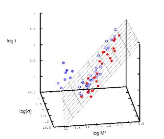
Figure 9: Left panel: Globular cluster efficiency (total number of clusters per stellar mass unit) as a function of stellar mass and projected stellar mass density ($\sigma$). Filled dots lie below the plane. Dots with a cross belong to the most massive galaxies. Right panel: Edge on view of the plane depicted in the previous figure, for galaxies with total stellar mass smaller than $10^{11}~{}M_{\odot}$.

This figure shows that most galaxies with stellar masses below $\approx 10^{11}$ $M_{\odot}$ define a thick plane. In turn, eight of the brightest galaxies appear clearly detached and above that plane. These last galaxies exhibit intermediate to low projected mass densities and, also, low central surface brightness compared to the Sérsic profile that fits the outer galaxy profile (see Kormendy et al. 2008). We point out that the t parameters listed in Table 4 for these galaxies are only approximate values. This is due to the fact that both GC families have cores in their spatial distribution (i.e. the projected GC density profiles are shallower than the galaxy brigtness profiles) leading to low t ratios in their inner regions. On the other side, as noted before, their total masses include a considerable fraction beyond a=150 arcsecs. A tentative correction for this last effect would increase their tabulated $log({\sigma})$ values by $\approx 0.25$.

A least square fit to the t values (in $10^{-9}$ units) and assuming no errors on effective radii or projected mass density, yields, for 49 galaxies with stellar masses smaller than $10^{11}M_{\odot}$:

$$log(t)=-0.70(\pm 0.05)~{}log(M_{*})+0.11(\pm 0.04)~{}log(\sigma)+$$

$$6.75(\pm 0.04)\$$ (13)

with a fit rms of $\pm 0.17$ in $log(t)$. The fit residuals in log(t) show no correlation with galaxy mass, integrated colour, morphology or position within the Virgo cluster.

An “edge-on” view of the plane is depicted in Figure 9 (right panel) excluding the eight brightest galaxies in Table 1.

The dependency with projected mass density becomes more evident if only the red GCs (in 31 bimodal galaxies), are included in the fit:

$$log(t_{red})=-0.65(\pm 0.16)~{}log(M_{*})+0.21(\pm 0.09)~{}log(\sigma)+$$

$$4.99(\pm 0.05)\$$ (14)

with a fit rms of $\pm 0.21$ in $log(t_{red})$.

On the other side, blue GC in 49 galaxies (31 with bimodal and 18 with unimodal GC systems) show a steeper slope with stellar mass but no detectable dependence with projected mass density:

$$log(t_{blue})=-0.91(\pm 0.07)~{}log(M_{*})+0.02(\pm 0.05)~{}log(\sigma)+$$

$$9.37(\pm 0.04)\$$ (15)

with a fit rms of $\pm$ 0.19 in $log(t_{blue})$.

This lack of dependency may be expected as the dominant stellar mass in bimodal GC galaxies appears associated with the red GC population according to Table 1.

10 Conclusions

The analysis presented in this work suggests that GC in early type galaxies are good tracers of their stellar populations. We stress that, the proposed GC formation efficiency dependence with chemical abundance, leads to a good approximation of the galaxy integrated colours and is consistent with a constant $\delta$ parameter suggesting a common pattern for the GC-field stars connection.

We also note, in particular, that this approach is able to explain the stellar halo-mean GC colour differences without implying definitely distinct formation histories for field stars and GC, although see Peng et al. (2008) for a different interpretation.

In turn, the inferred galaxy $(M/L)_{B}$ ratios compare well with the range of values found in the literature and seem consistent with old ages and small formation time spreads.

The on-set of GC colour bimodality seems to occur at masses larger than $M_{*}\approx 10^{10}M_{\odot}$, i.e., galaxies with lower masses only give rise to blue GC. Interestingly, Dekel & Woo (2003) suggest that galaxies with masses smaller than $\approx 3.10^{10}M_{\odot}$ are efficiently cleaned of interstellar matter as a result of stellar and SNe winds leading to an interruption of the star formation process.

The two dominant GC families have rather distinct characteristics. On one side, “blue” globulars can be characterized by a very low chemical abundance spread suggesting that some kind of major common event may have played a role in their “synchronous” formation and relatively homogeneous chemical composition. The re-ionization of the Universe has been put forward as possible responsible for this characteristic (e.g. Santos 2003) although the impact of re-ionization on galaxy and galaxy-cluster scales should also deserve further analysis. In any case, the increase of $Zs(blue)$ with galaxy mass lends support to the idea that blue GC in fact “know” about the galaxy they are related to (e.g. Strader, Brodie & Forbes 2004).

The very narrow metallicity scale of the blue GC is compatible with their formation in low effective-yield environments characterized by important mass loss leading to a rapid supression of field star formation (e.g. Harris et al. 2006) and to high GC formation efficiencies.

In turn, red clusters exhibit an abundance spread that becomes larger for more massive galaxies and appear associated, when GC bimodality is observable, with the dominant stellar mass component. This is coherent with the idea that more massive systems exhibit higher mean chemical abundances. The large dispersion of the relation between the $Zs(red)$ scale and galaxy mass may be also indicating some diversity in the formation history of this component (e.g. different numbers of mergers and their effects on gas removal).

The overall increase of chemical abundance with mass derived in this work, is consistent with the GC formation modelling presented by Bekki et al. (2008). These models imply a formation time spread of roughly 3 Gy (i.e. $\pm$ 1.5 Gy around a mean value of about 11 Gyr.

We also stress that the broad behaviour derived for t with galaxy mass is coherent with the starting hypothesis in this work, i.e., that the number of clusters per diffuse stellar mass unit increases with decreasing metallicity (and hence with decreasing stellar mass according to the stellar mass-metallicity relation).

In more detail, galaxies with stellar masses lower that $M_{*}\approx 10^{11}M_{\odot}$ define a thick plane in the logarithmic stellar mass-$\sigma$-t space where the GC formation efficiency seem dependent on both galaxy mass and projected surface mass density. Such a dependence becomes more evident when only red GC are taken into consideration. This result resembles those by Larsen & Richtler (2000) who suggest a dependence of the formation of young and massive stellar cluster with projected mass density. The lack of such a dependence in the case of the blue GC reinforces the idea that these clusters have genetic differences with the red ones.

Remarkably, the most massive galaxies in the sample appear clearly detached and above that plane. Naively, this is the expected situation for galaxies suffering mergers, although a number of dynamical effects that may have an impact on the t parameter still remain to be considered before adopting this conclusion. For example, in the case of (dry) merging two galaxies with similar masses and GC populations, the composite t parameter would remain unchanged while the total mass would be doubled. These massive galaxies also exhibit large effective radii and intermediate projected stellar mass densities, a signature of major merger events (e.g. Shin & Kawata 2009).

A tentative conclusion, that will deserve further analysis, suggests that galaxies with stellar masses below that value, and located on the “thick” plane described in this paper, may have suffered a relatively small number of disippationless merging events along their life. This conclusion also gets support from CDM based modelling (e.g. De Lucía et al. 2007) showing that less massive galaxies may have had a low number of galaxy-progenitors in their formation history.

Appendix:GC colour histograms

GC colour histogram fits for 63 galaxies (*) in the Virgo ACS. Heavy black lines are the (background corrected) observed histograms. Red lines show the histograms that give the best fits in terms of the quality indicator (see Table 1). Dots show the counting uncertainties for each colour bin. Note that Figure 4, in this paper, only shows nine representative histogram fits.

(*) In the print version of the journal, the figures for only the first 12 galaxies are included. The figures for all 63 galaxies can be found in the online version.

References

- Beasley et al. (2002) Beasley M. A., Baugh C.M., Forbes D.A., Sharples R.M., Frenk C. S., 2002, MNRAS, 333, 383
- Beasley et al. (2008) Beasley M. A., Bridges T., Peng E., Harris W.E., Harris G.L.H., Forbes D.A., Mackie G, 2008, MNRAS, 386, 1443
- Bekki et al. (2008) Bekki, B. Yahagi H., Nagashima M., Forbes D.A., 2008, MNRAS 387, 1131
- Binggeli, Sandage & Tammann (1985) Binggeli, B., Sandage A., Tammann G.A., 1985, AJ, 90, 1681
- Brodie & Strader (2006) Brodie J.P., Strader J. 2006, AR&A 44, 193
- Bruzual & Charlot (2003) Bruzual G., Charlot S., 2003, MNRAS 344, 1000
- Caon et al. (1990) Caon N., Capaccioli M., Rampazzo R., 1990, MNRAS, 242, 24
- Chabrier ((2003)) Chabrier G., 2003, PASP 115, 763
- Charlton & Laguna (1995) Charlton J.C., Laguna P., 1995, ApJ, 444, 193
- Côté et al. (1998) Côté P. Marzke R. O., West M. J., 1998, ApJ, 501, 554
- Côté et al. (2004) Côté P., Blakeslee J.P., West M. J., Ferrarese, L., Jordán A., Mei S., Merritt D., Milosavljević M., Peng E.W., Tonry J. L., West M. J., 2004, ApJS, 153, 223
- De Lucía et al. (2007) De Lucía G., Springel V., White S.D.M., Croton D., Kauffman G., 2006, MNRAS, 366, 499
- Dekel & Woo (2003) Dekel A., Woo J., 2003, MNRAS, 368, 2
- Eggen, Lynden Bell & Sandage ((1962)) Eggen O., Lynden Bell D., Sandage A.R., 1962, ApJ, 136, 748
- Ferrarese et al. (2006) Ferrarese L., Côté P.,Jordán A., Peng E.W., Blakeslee J.P., Piatek S., Mei S., Merritt D., Milosavljević M., Tonry, J. L., West M. J., 2006, ApJS, 164, 334
- Forbes et al. (2001) Forbes D. A., Beasley M.A., Brodie J.P., Kissler-Patig M., 2001, ApJ, 563, 143
- Forbes & Forte ((2001)) Forbes D. A., Forte, J.C., 2001, MNRAS, 322, 257
- Forte, Strom & Strom ((1981)) Forte J.C., Strom S. E., Strom K., 1981, ApJ, 245, L9
- Forte et al. (2001) Forte J.C., Geisler D., Ostrov P.G., Piatti A.E., Gieren W., 2001, AJ, 121, 1992
- Forte, Faifer & Geisler ((2005)) Forte J.C., Faifer F., Geisler D., 2005, MNRAS, 357, 56
- Forte, Faifer & Geisler ((2007)) Forte J.C., Faifer F., Geisler D., 2007, MNRAS, 382, 1947
- Gnedin & Ostriker (1997) Gnedin O.Y., Ostriker J.P., 1997, 474, 223
- Harris & van den Bergh (1981) Harris W.E., van den Bergh S., 1981, AJ, 86, 1627
- Harris et al. (2006) Harris W.E., Whitmore B.C., Karakla D., Okon W., Baum W.A., Hanes D.A., Kavelaars D.J., 2006, ApJ, 636,90
- Hempel et al. (2007) Hempel M., Kissler-Patig M., Puzzia T.H., Hilker M., 2007, A&A, 463, 493
- Janz & Lisker (2009) Janz J., Lisker T., arXiv 0903.5301v1
- Kauffmann et al. (2003) Kauffmann, G. et al. 2003, MNRAS 341, 33
- Kodama et al. (1998) Kodama T. et al. 1998, A&A, 334, 99
- Kormendy et al. (2008) Kormendy J., Fisher D.B., Cornell M.E., Bender R., 2008, arXiv 0810.1681
- Kundu & Zepf (2007) Kundu A., Zepf, S.E., 2007, ApJ, 660, L109
- Kundu ((2008)) Kundu A., 2008, AJ 136, 1013
- La Barbera et al. (2008) La Barbera F., Busarello G., Merluzzi P., De la Rosa I., Cóppola G., Haines C.P., 2008, ApJ (accepted) astro-ph 0807.3829
- Larsen & Richtler (2000) Larsen S. S., Richtler T., 2000, A&A, 354, 836
- Maraston (2005) Maraston C., 2005, MNRAS, 362, 799
- Mendel, Proctor & Forbes (2007) Mendel J. T., Proctor R. N., Forbes D. A., 2007, MNRAS, 379, 1618
- Michard (2000) Michard, R., 2000, A&A 360, 85
- Mieske et al. (2006) Mieske, S. et al.,2006, ApJ, 653,193
- Miller & Lotz (2007) Miller B.W., Lotz J., 2007, ApJ, 670, 1074
- Napolitano et al. (2005) Napolitano N.R., Capaccioli A.J., Romanowsky A.J., Douglas N.G., Merrifield M.R., Kuijken K., Arnaboldi M., Gerhard O., Freeman K.C., 2005, MNRAS, 357, 691
- Norris et al. ((2008)) Norris M.A., Sharples R. M., Bridges T., Gebhardt K., Forbes D. A., Proctor R., Faifer F., Forte J.C., Beasley M.A., Zepf S. E., Hanes D.A., 2008, MNRAS 385, 40
- Ostrov, Geisler & Forte (1993) Ostrov P.G., Geisler, D., Forte, J.C., 1993, AJ, 105, 1762
- Peng et al. (2006) Peng E. W., et al., 2006, ApJ, 639, 838
- Peng et al. ((2008)) Peng E. W., et al., 2008, ApJ, 681, 197
- Pierce et al. (2006a) Pierce M., Beasley M. A., Forbes D. A., Bridges T., Gebhardt K., Faifer F. R., Forte J. C., Zepf, S. E. Sharples R., Hanes D. A., Proctor R., 2006a, MNRAS 366, 1253
- Pierce et al. (2006b) Pierce M., Bridges T., Forbes D. A., Proctor R., Beasley M. A., Gebhardt K., Faifer F. R., Forte J. C., Zepf S. E., Sharples R., Hanes D. A., 2006b, MNRAS 368, 325
- Rhode, Zepf & Santos (2005) Rhode K.L., Zepf S.E., Santos M.R., 2005, ApJ 630, L2
- Rodgers et al. (2006) Rodgers C. T., Canterna R., Smith J.A., Pierce M.J., Tucker D.L., 2006, AJ, 132, 989
- Santos (2003) Santos M.R., 2003, in Extragalactic Globular Cluster Systems, ed. M. Kissler-Patig (New York: Springer Verlag)
- Schlegel et al. (1998) Schlegel D., Finkbeiner D., Davis M., 1998, ApJ, 500,525
- Searle & Zinn ((1978)) Searle L., Zinn R., 1978, ApJ, 205, 357
- Shin & Kawata (2009) Shin M-S.,Kawata D., 2009, ApJ, 691, 83
- Spitler et al. (2008) Spitler L.R., Forbes D.A., Strader J., Brodie J.P., Gallagher J.S., 2008, MNRAS, 385,361
- Strader et al. (2007) Strader J., Beasley M.A., Brodie, J.P., 2007, AJ, 133, 2015
- Strader et al. (2004) Strader J., Brodie J. P., Forbes D. A., 2004, AJ, 127, 295
- Strader, Brodie & Forbes (2004) Strader J., Brodie J. P., Forbes D. A., 2004, AJ, 127, 3431
- Strader et al. (2006) Strader J., Brodie J. P., Spitler M., Beasley M.A., 2006, AJ, 132, 2333
- Thomas et al. (2004) Thomas D., Maraston C., Korn A., 2004, MNRAS, 351, L19
- Thomas et al. (2005) Thomas D., et al., 2005, 2005, ApJ, 621, 673
- Tonry et al. (2001) Tonry T., Dressler A., Blakeslee J.P., Ajhar E.A., Fletcher A.B, Luppino G.A., Metzger M.R., Moore C.B., 2001, ApJ, 546, 681
- Waters et al. ((2008)) Waters C.Z., Zepf S.E., Lauer T., Baltz E.A., arXiv0811.0391
- Worthey (1994) Worthey G., 1994, ApJS, 95, 107
- Zepf & Ashman (1993) Zepf, S.E., MNRAS 264, 611
- Zinn & West (1984) Zinn R., West M. J., 1984, ApJS, 55, 45
- Zepf & Ashman (1993) Zepf S. E., Ashman K. M., 1993, MNRAS, 264, 611