Sparse Poisson Intensity Reconstruction Algorithms

Abstract

The observations in many applications consist of counts of discrete events, such as photons hitting a dector, which cannot be effectively modeled using an additive bounded or Gaussian noise model, and instead require a Poisson noise model. As a result, accurate reconstruction of a spatially or temporally distributed phenomenon ($f$) from Poisson data ($y$) cannot be accomplished by minimizing a conventional $\ell_{2}-\ell_{1}$ objective function. The problem addressed in this paper is the estimation of $f$ from $y$ in an inverse problem setting, where (a) the number of unknowns may potentially be larger than the number of observations and (b) $f$ admits a sparse approximation in some basis. The optimization formulation considered in this paper uses a negative Poisson log-likelihood objective function with nonnegativity constraints (since Poisson intensities are naturally nonnegative). This paper describes computational methods for solving the constrained sparse Poisson inverse problem. In particular, the proposed approach incorporates key ideas of using quadratic separable approximations to the objective function at each iteration and computationally efficient partition-based multiscale estimation methods.

Index Terms—  ​​​ Photon-limited imaging, Poisson noise, wavelets, convex optimization, sparse approximation, compressed sensing

1 Introduction

In a variety of applications, ranging from nuclear medicine to night vision and from astronomy to traffic analysis, data are collected by counting a series of discrete events, such as photons hitting a detector or vehicles passing a sensor. The measurements are often inherently noisy due to low count levels, and we wish to reconstruct salient features of the underlying phenomenon from these noisy measurements as accurately as possible. The inhomogeneous Poisson process model [1] has been used effectively in many such contexts. Under the Poisson assumption, we can write our observation model as

$$y\sim{{\rm Poisson}}(Af),$$ (1)

where $f\in\mathbb{R}_{+}^{m}$ is the signal or image of interest, $A\in\mathbb{R}_{+}^{N\times m}$ linearly projects the scene onto a $N$-dimensional set of observations, and $y\in{\mathbb{Z}}_{+}^{N}$ is a length-$N$ vector of observed Poisson counts.

The problem addressed in this paper is the estimation of $f$ from $y$ in a compressed sensing context, when (a) the number of unknowns, $m$, may be larger than the number of observations, $N$, and (b) $f$ is sparse or compressible in some basis $W$ (i.e. $f=W\theta$ and $\theta$ is sparse). This challenging problem has clear connections to “compressed sensing” (CS) (e.g., [2]), but arises in a number of other settings as well, such as tomographic reconstruction in nuclear medicine, superresolution image reconstruction in astronomy, and deblurring in confocal microscopy.

In recent work [3], we explored some of the theoretical challenges associated with CS in a Poisson noise setting, and in particular highlighted two key differences between the conventional CS problem and the Poisson CS problem:

1. unlike many sensing matrices in the CS literature, the matrix $A$ must contain all nonnegative elements, and

2. the intensity $f$, and any estimate of $f$, must be nonnegative.

Not only are these differences significant from a theoretical standpoint, but they pose computational challenges as well. In this paper, we consider algorithms for computing as estimate $\widehat{f}$ of $f$ from observations $y$ according to

$$\widehat{f} \triangleq \mathop{\arg\min}_{\widetilde{f}\in\Gamma}-\log\ p\!\left(y\left|A\widetilde{f}\right.\right)+{\rm pen}(\widetilde{f}\,)$$

$$= \mathop{\arg\min}_{\widetilde{f}\in\Gamma}\sum_{i=1}^{N}\left\{\left(A\widetilde{f}\,\right)_{i}-y_{i}\log\left[\left(A\widetilde{f}\,\right)_{i}\right]\right\}+{\rm pen}(\widetilde{f}\,),$$

where

• $p\!\left(y\left|A\widetilde{f}\right.\right)$ is the Poisson likelihood of $y$ given intensity $A\widetilde{f}$,

• $\left(A\widetilde{f}\,\right)_{i}$ is the $i^{\rm th}$ element of the vector $A\widetilde{f}$,

• $\Gamma$ is a collection of nonnegative estimators such that $\widetilde{f}\geq 0$ for all $\widetilde{f}\in\Gamma$, and

• ${\rm pen}(\widetilde{f}\,)$ is a penalty term which measures the sparsity of $\widetilde{f}$ in some basis.

This paper explores computational methods for solving (1). The nonnegativity of $f$ and $A$ results in challenging optimization problems. In particular, the restriction that $f$ is nonnegative introduces a set of inequality constraints into the minimization setup; as shown in [4], these constraints are simple to satisfy when $f$ is sparse in the canonical basis, but they introduce significant challenges when enforcing sparsity in an arbitrary basis. We will consider several variants of the penaly term, including $\|f\|_{1}$, $\|W^{T}\!\!f\|_{1}$ for some arbitrary orthonormal basis $W$, and a complexity regularization penalty based upon recursive dyadic partitions. We refer to our approach as SPIRAL (Sparse Poisson Intensity Reconstruction ALgorithm).

The paper is organized as follows. We first consider related optimization methods for solving the compressed sensing problem in Sec. 2. Next, in Sec. 3, we consider three methods for solving the constrained penalized Poisson likelihood estimation problem with different penalty terms. The first two approaches use an $\ell_{1}$ penalty while the third uses partition-based penalty functions. Experimental results comparing the proposed approaches with expectation-maximization (EM) algorithms are presented in Sec. 4.

2 Sparsity-regularized optimization

Without any nonnegativity constraints on $f$, the Poisson minimization problem (1) can be solved using the SpaRSA algorithm of Figueireido et al. [5], which solves a sequence of minimization problems using quadratic approximations to the log penalty function:

$$f^{k+1}\triangleq\underset{f\in\mathbb{R}^{m}}{\arg\min}\ \ \frac{1}{2}\|f-s^{k}\|_{2}^{2}+\frac{1}{\alpha_{k}}{\rm pen}(f),$$ (2)

where

$$s^{k}=f^{k}-\frac{1}{\alpha_{k}}\nabla F(f^{k}),$$ (3)

$\alpha_{k}$ is a positive scalar chosen using Barzilai-Borwein (spectral) methods (see [5] for details), and

$$F(f)\triangleq-\log p(y|Af)$$

is the negative log Poisson likelihood in (1). If the penalty term in (2) is separable, i.e., it is the sum of functions with each function depending only on one component of $f$, then (2) can be solved component-wise, making the problem (2) relatively easy to solve.

Much of existing CS optimization literature (e.g., [6, 7, 8]) focuses on penalty functions where ${\rm pen}(f)\propto\|W^{T}\!\!f\|_{1}$, where $W$ is some orthonormal basis, such as a wavelet basis, and $\theta\triangleq W^{T}\!\!f$ are the expansion coefficients in that basis. Also, nonnegativity in the signal $f=W\theta\geq 0$ is not necessarily enforced. In this paper, we develop three approaches to solving the optimization problem in (1). In all three approaches, we require $f$ to be nonnegative. The first approach assumes that the image is sparse in the canonical basis, i.e., $W=I$, while the second involves the more general orthogonal matrix $W$. The third uses partition-based denoising methods, described in detail in Sec. 3.3.

3 nonnegative regularized least-squares subproblem

3.1 Sparsity in the canonical basis

Let ${\rm pen}(f)=\tau\|f\|_{1}$, where $\tau>0$ is a regularization parameter. The minimization problem (2) with this penalty term and that is subject to nonnegativity constraints on $f$ has the following analytic solution:

$$f^{k+1}=\left[s^{k}-\frac{\tau}{\alpha_{k}}\mathbbm{1}\right]_{+}$$

where the operation $[\enspace\cdot\enspace]_{+}=\max\{\ \cdot\ ,0\}$ is to be understood component-wise. Thus solving (1) subject to nonnegativity constraints with an $\ell_{1}$ penalty function and with a solution that is sparse in the canonical basis is straightforward to solve. An alternative algorithm for solving this Poisson inverse problem with sparsity in the canonical basis was also explored in the recent literature [4].

3.2 Sparsity in an arbitrary orthonormal basis

Now suppose that the signal of interest is sparse in some other basis. Then the $\ell_{1}$ penalty term is given by

$${\rm pen}(f)\triangleq\tau\|W^{T}\!\!f\|_{1}=\tau|\theta\|_{1},$$

where $\theta\triangleq Wf$ for some orthonormal basis $W$, and $\tau>0$ is some scalar. When the reconstruction $\hat{f}=W\hat{\theta}$ must be nonnegative (i.e., $W\hat{\theta}\geq 0$), the minimization problem

$$\theta^{k+1}\triangleq\ \underset{\theta\in\mathbb{R}^{m}}{\arg\min}\quad\phi^{k}(\theta)\triangleq\frac{1}{2}\|\theta-s^{k}\|_{2}^{2}+\frac{\tau}{\alpha_{k}}\|\theta\|_{1},$$

$$\textrm{subject to \ }W\theta\geq 0$$ (4)

no longer has an analytic solution necessarily. We can solve this minimization problem by solving its dual. First, we reformulate (4) so that its objective function $\phi^{k}(\theta)$ is differentiable by defining $u,v\geq 0$ such that $\theta=u-v$. The minimization problem (4) becomes

$$(u^{k+1},v^{k+1})\triangleq\ \underset{u,v\in\mathbb{R}^{m}}{\arg\min}\quad\frac{1}{2}\|u-v-s^{k}\|_{2}^{2}+\frac{\tau}{\alpha_{k}}\mathbbm{1}^{T}\!(u+v)$$

$$\textrm{subject to \ }u,v\geq 0,\quad W(u-v)\geq 0,$$ (5)

which has twice as many parameters and has additional nonnegativity constraints on the new parameters, but now has a differentiable objective function. The Lagrange dual problem associated with this problem is given by

$$\underset{\lambda,\gamma\in\mathbb{R}^{m}}{\textrm{minimize}}\ \ h(\lambda,\gamma)\triangleq\frac{1}{2}\|s^{k}+\gamma+W^{T}\!\lambda\|_{2}^{2}-\frac{1}{2}\|s^{k}\|_{2}^{2}\quad$$

$$\textrm{subject to \ }\lambda\geq 0,\ \ \ -\frac{\tau}{\alpha_{k}}\mathbbm{1}\leq\gamma\leq\frac{\tau}{\alpha_{k}}\mathbbm{1}$$ (6)

and at the optimal values $\gamma^{\star}$ and $\lambda^{\star}$, the primal iterate $\theta^{k+1}\triangleq u^{k+1}-v^{k+1}$ is given by

$$\theta^{k+1}=s^{k}+\gamma^{\star}+W^{T}\!\lambda^{\star}.$$

We note that the minimizers of the primal problem (5) and its dual (6) satisfy $\phi^{k}(\theta^{k+1})=-h(\gamma^{\star},\lambda^{\star})$ since (5) satisfies (a weakened) Slater’s condition [9]. In addition, the function $-h(\gamma,\lambda)$ is a lower bound on $\phi^{k}(\theta)$ at any dual feasible point.

The objective function of (6) can be minimized by alternatingly solving for $\lambda$ and $\gamma$, which is accomplished by taking the partial derivatives of $h(\lambda,\gamma)$ and setting them to zero. Each component is then constrained to satisfy the bounds in (6). At the $j^{\rm th}$ iteration, the variables can, thus, be defined as follows:

$$\gamma^{(j)}\!\!\! = \!\!\textrm{mid}\left\{-\frac{\tau}{\alpha_{k}}\mathbbm{1},-s^{k}-W^{T}\!\lambda^{(j-1)},\frac{\tau}{\alpha_{k}}\mathbbm{1}\right\}$$

$$\lambda^{(j)}\!\!\! = \!\!\left[-W\left(s^{k}+\gamma^{(j)}\right)\right]_{+},$$

where the operator mid($a,b,c$) chooses the middle value of the three arguments component-wise. Note that at the end of each iteration $j$, the approximate solution $\theta^{(j)}\triangleq s^{k}+\gamma^{(j)}+W^{T}\lambda^{(j)}$ to (4) is feasible with respect to the constraint $W\theta\geq 0$:

$$W\theta^{(j)} = Ws^{k}+W\gamma^{(j)}+\lambda^{(j)}$$

$$= \left[W\left(s^{k}+\gamma^{(j)}\right)\right]_{+}\geq 0.$$

Unfortunately, there are several important disadvantages associated with the above approach. First, the solution to the subproblem must itself be computed by an iterative algorithm – so while the problem may be solvable, it must by solved at each iterate, and the resulting overall algorithm may not be fast, particularly for large problems. Furthermore, since we rely on an iterative solver in this subproblem, our computed solution may not be the true optimal point, particularly if we use a gentle convergence requirement to limit computation time. Further study is needed to understand the impact of computing inaccurate solutions to this subproblem on the performance of the overall algorithm.

3.3 Partition-based penalties

In the special case where the signal of interest is known to be smooth or piecewise smooth in the canonical basis (i.e. is compressible in a wavelet basis), we can formulate a penalty function which is a useful alternative to the $\ell_{1}$ norm of the wavelet coefficient vector. In particular, we can build on the framework of recursive dyadic partitions (RDP), which we summarize here and are described in detail in [10, 11]. Let $\mathcal{P}$ be the class of all recursive dyadic partitions of $[0,1]$ where each interval in the partition has length at least $1/m$, and let $P\in\mathcal{P}$ be a candidate partition. The intensity on $P$, denoted $f(P)$, is calculated using a nonnegative least-squares method to fit a model (such as a constant or polynomial) to $s^{k}$ in (3) on each interval in the RDP. Furthermore, a penalty can be assigned to the resulting estimator which is proportional to $|P|$, the number of intervals in $P$. Thus we set

$$\widehat{P} =\mathop{\arg\min}_{P\in\mathcal{P}}\frac{1}{2}\|f(P)-s^{k}\|_{2}^{2}+\tau|P|$$

$$\widehat{f} =f(\widehat{P}).$$

A search over $\mathcal{P}$ can be computed quickly using a dynamic program. When using constant partition interval models , the nonnegative least-squares fits can be computed non-iteratively in each interval by simply using the maximum of the average of $s^{k}$ in that interval and zero. Because of this, enforcing the constraints is trivial and can be accomplished very quickly.

It can be shown that partition-based denoising methods such as this are closely related to Haar wavelet denoising with an important hereditary constraint placed on the thresholded coefficients—if a parent coefficient is thresholded, then its children coefficients must also be thresholded [10]. This constraint is akin to wavelet-tree ideas which exploit persistence of significant wavelet coefficients across scales and have recently been shown highly useful in compressed sensing settings [12].

As we mention in Sec. 4 below, using constant model fits makes it easy to satisfy nonnegativity constraints and results in a very fast non-iterative algorithm, but has the disadvantage of yielding piecewise constant estimators. However, a cycle-spun translation-invariant version of this approach can be implemented with high computational efficiency [10] and be used for solving this nonnegative regularized least-squares subproblem that results in a much smoother estimator.

4 Numerical simulations

We evaluate the effectiveness of the proposed approaches in reconstructing a piecewise smooth function from noisy compressive measurements. In our simulations, the true signal (the black line in Figs. 1(a–c)) is of length 1024. We take 512 noisy compressive measurements of the signal using a sensing matrix that contains 32 randomly distributed nonzero elements per row. This setup yields a mean detector photon count of 50, ranging from as few as 22 photons, to as high as 94 photons. We allowed each algorithm a fixed time budget of three seconds in which to run, which is sufficient to yield approximate convergence for all methods considered. Each algorithm was initialized at the same starting point, which was generated using a single E-step of the EM algorithm. That is if $z=A^{T}y$, and $x:x_{i}=y_{i}/(Az)_{i}$, then we initialize with $f^{0}:f_{i}^{0}=z_{i}(A^{T}x)_{i}/(A^{T}\mathbbm{1})_{i}$. The value of the regularization parameter $\tau$ was tuned independently for each algorithm to yield the minimal root-mean-squared error $\text{RMS}=\|\hat{f}-f\|_{2}/\|f\|_{2}$ at the exhaustion of the computation budget (see Table 1).

Reconstruction Method	RMS
SPIRAL (TI)	0.1427
SPIRAL (TV)	0.1855
EM-MPLE (TI)	0.2485
EM-MPLE (TV)	0.2511
SPIRAL ($\ell_{1}$)	0.2898

Table 1: Reconstruction accuracy as measured by the root-mean-squared error, $\text{RMS}=\|\hat{f}-f\|_{2}/\|f\|_{2}$.

An examination of the results in Figs. 1(a-c) reveals that even though models within a partition (constant pieces) are less smooth than higher-order wavelets, this drawback is neutralized through a combination of cycle spinning (TI), the hereditary constraint, and a fast, non-iterative solver. We compare our algorithm with an EM algorithm based upon the same maximum penalized likelihood estimation (MPLE) objective function proposed in (1), which has been used previously in imaging contexts in which sparsity in a multiscale partition-based framework was exploited [13]. Although Fig. 1(d) shows that the convergence behavior of the EM-MPLE approaches is more stable, their slow convergence ultimately hinders their performance as compared with the corresponding SPIRAL-based approaches. In the case of SPIRAL-$\ell_{1}$, the estimate seems very oscillatory; a smoother estimate could be achieved by increasing the regularization parameter $\tau$, but this leads to an “oversmoothed” solution and increases the RMS of the estimate. The large RMS values early in the SPIRAL iterations are due to small values of $\alpha_{k}$ when defining $s^{k}$ in (3), which occur when the estimates are flat and the consecutive iterates only change slightly. The Barzilai-Borwein method [7], on which the choice of $\alpha_{k}$ is based, is not monotone and can exhibit spikes in the iterates’ RMS values (the non-monotone SpaRSA algorithm is also not immune to this behavior, for example). Although it is difficult to characterize the convergence of this approach, it has been shown to be effective in solving minimization problems (see [7] for details). The SPIRAL partition-based estimates appear to oscillate in steady state. This effect could be mitigated by forcing the objective function to decrease monotonically with iteration, as described in [5] and as in EM algorithms. However, empirically this appears to hinder performance, as convergence is significantly slowed. We are currently investigating methods that use a non-monotonic approach to obtain a good approximation to the minimizer, followed by a monotonic method to enforce convergence.

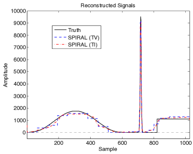
(a)	(b)
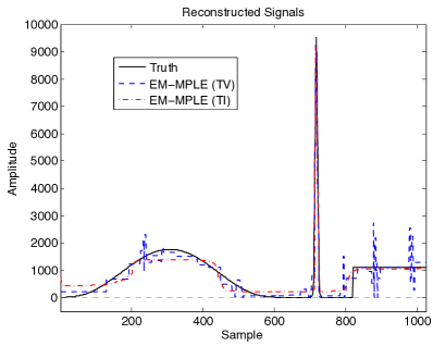
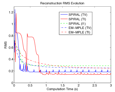
(c)	(d)

Fig. 1: Reconstruction results using(a) the SPIRAL algorithm with translationally variant (TV) and translationally invariant (TI) partitions, (b) the SPIRAL algorithm with an $\ell_{1}$ penalty, and (c) the EM-MPLE algorithm with translationally variant (TV) and translationally invariant (TI) partitions, (d) mean-squared error decay as a function of compute time.

5 Conclusion

We have developed computational approaches for signal reconstruction from photon-limited measurements—a situation prevalent in many practical settings. Our method optimizes a regularized Poisson likelihood under nonnegativity constraints. We have demonstrated that these methods prove effective in the compressed sensing context where an $\ell_{1}$ penalty is used to encourage sparsity of the resulting solution. Our method improves upon current approaches in terms of reconstruction accuracy and computational efficiency. By employing model-based estimates that utilize structure in the coefficients beyond that of a parsimonious representation, we are able to achieve greater accuracy with less computational burden. Future work includes supplementing our algorithms with a debiasing stage, which maximizes the likelihood over the sparse support discovered in the main algorithm. We also will be exploring the efficacy of alternative optimization approaches such as sequential quadratic programming and interior-point methods.

References

- [1] D. Snyder, Random Point Processes, Wiley-Interscience, New York, NY, 1975.
- [2] E. J. Candès and T. Tao, “Decoding by linear programming,” IEEE Trans. Inform. Theory, vol. 15, no. 12, pp. 4203–4215, 2005.
- [3] R. Willett and M. Raginsky, “Performance bounds for compressed sensing with Poisson noise,” in IEEE Int. Symp. on Inf. Theory, 2009, Accepted.
- [4] D. Lingenfelter, J. Fessler, and Z. He, “Sparsity regularization for image reconstruction with Poisson data,” in Proc. SPIE Computational Imaging VII, 2009, vol. 7246.
- [5] S. Wright, R. Nowak, and M. Figueiredo, “Sparse reconstruction by separable approximation,” IEEE Trans. Signal Process., 2009 (to appear).
- [6] S.-J. Kim, K. Koh, M. Lustig, S. Boyd, and D. Gorinevsky, “A method for large-scale l1-regularized least squares,” IEEE J. Sel. Top. Sign. Process., vol. 1, no. 4, pp. 606–617, 2007.
- [7] M. Figueiredo, R.D. Nowak, and S.J. Wright, “Gradient projection for sparse reconstruction: Application to compressed sensing and other inverse problems,” IEEE J. Sel. Top. Sign. Process., vol. 1, no. 4, pp. 586, 2007.
- [8] W. Yin, S. Osher, D. Goldfarb, and J. Darbon, “Bregman iterative algorithms for l1-minimization with applications to compressed sensing,” SIAM J. Imag. Sci., vol. 1, no. 1, pp. 143–168, 2008.
- [9] S. Boyd and L. Vandenberghe, Convex optimization, Cambridge University Press, Cambridge, 2004.
- [10] R. Willett and R. Nowak, “Multiscale Poisson intensity and density estimation,” IEEE Trans. Inform. Theory, vol. 53, no. 9, pp. 3171–3187, 2007.
- [11] R. Nowak, U. Mitra, and R. Willett, “Estimating inhomogeneous fields using wireless sensor networks,” IEEE J. Sel. Areas Commun., vol. 22, no. 6, pp. 999–1006, 2004.
- [12] R. Baraniuk, V. Cevher, M. F. Duarte, and C. Hegde, “Model-based compressive sensing,” Submitted, 2009.
- [13] R. Willett and R. Nowak, “Platelets: a multiscale approach for recovering edges and surfaces in photon-limited medical imaging,” IEEE Transactions on Medical Imaging, vol. 22, no. 3, pp. 332–350, 2003.