Tree-level Split Helicity Amplitudes in Ambitwistor Space

Abstract:

We study all tree-level split helicity gluon amplitudes by using the recently proposed BCFW recursion relation and Hodges diagrams in ambitwistor space. We pick out the contributing diagrams and find that all of them can be divided into triangles in a suitable way. We give the explicit expressions for all of these amplitudes. As an example, we reproduce the six gluon split NMHV amplitudes in momentum space.

1 Introduction

There are a lot of hidden elegant structures in tree-level amplitudes in Yang-Mills theory. These structures cannot be seen from the standard Feynman rules directly. One typical example is the Parke-Taylor formula for the MHV amplitudes [1] which was later proved in [2]. In 2003, by transforming the amplitudes into twistor space, Witten found a beautiful explanation of the simplicity of these amplitudes[3]. He furthermore proposed a dual topological B model in super twistor space ${\bf CP}^{3|4}$ to calculate the tree-level amplitudes. Being different from the usual strong-weak duality in AdS/CFT correspondence, his proposal is a kind of weak-weak duality. Moreover, the study of this twistor string theory inspired the development of a new computation formalism - MHV diagrams [4] (also known as CSW rules) in which off-shell continuations of MHV amplitudes is used as vertices to build up the diagrams. Later on an on-shell recursion relation was proposed in [5, 6]. This so-called BCFW recursion relation is a very powerful computation tool at tree level. Last year, all tree-level amplitudes in ${\cal N}=4$ super Yang-Mills theory and ${\cal N}=8$ supergravity were computed in [7] and [8] by using the maximal supersymmetric version [9, 10] of BCFW relation.

Recently, it was revealed that there were more surprises in the amplitudes of (super-)Yang-Mills and (super-)gravity in (ambi)-twistor space[11, 12]. Especially, in [12] it was shown that all tree amplitudes could be combined into an “S-matrix” scattering functional in twistor space. The on-shell (super-)BCFW relation in ambitwistor space (using both twistor and dual twistor) plays an essential role in their study. In the (ambi-)twistor space, the relation turns out to be simpler and more elegant. In [12], a diagrammatic representation was also given for this recursion relation. Using the BCFW formula, the multiparticle amplitudes could be represented by a set of diagrammatic rule, which actually gave a concrete realization of Penrose’s “twistor diagram program” [13, 14]. In fact, the twistor diagram formalism in [12] is a refined version of the formalism developed by Hodges in [15, 16, 17]. It turns out that considering amplitudes in (ambi-)twistor space could not only make the computation much easier but also uncover the underlying structure in Yang-Mills theory.

Among all of the tree-level gluon (partial) amplitudes, the class of split helicity amplitudes is of particular interest. In these amplitudes, the gluons with the same helicity are put together. The amplitudes in this class are closed under the original BCFW recursion relations for gluon amplitudes [5]. These amplitudes have been computed in momentum space [18] by solving these recursion relations. In [19], it has been shown that they are also dual conformal covariant. In this paper, we will study these amplitudes in ambitwistor space.

The main tools we will use are the BCFW relation and the Hodges diagrams developed in [12]. One of the key points in our computation is the following: due to the Grassman integration used to pick out the gluon amplitude from the superamplitudes, many Hodges diagrams do not really contribute so that they could be thrown away. This idea simplifies the computation significantly. By investigating some simple examples, we come to the conclusion that each of the remaining Hodges diagram can be divided into triangles in a suitable way. These triangles are naturally combined into some domains. Besides the MHV ($\overline{MHV}$) domains discussed in [20, 21], there is another new kind of domains which we name as “type II” domains. One of the differences between these two kinds of domains is the helicities of the external gluon of the domains. Using these domains, we can write down all of the expressions for the split helicity amplitudes. We also check that our result reproduce the six gluon split helicity next-to-MHV (NMHV) amplitude.

In the next section of this paper, we will give a brief introduction to the BCFW recursion relation in ambitwistor space and the Hodges diagrams in [12]. We will study the split helicity amplitudes in section 3. After some general discussions in subsection 3.1, we will first study split MHV amplitudes in subsection 3.2. We then study two examples with few external gluons in subsection 3.3. We give our general results for split helicity amplitudes in subsection 3.4. In section 4, we show that we reproduce the six-gluon split helicity NMHV amplitudes in momentum space. The final section is devoted to conclusion and discussions.

2 BCFW recursion relation in ambitwistor space

The on-shell momentum of external gluon $p^{\mu}$ can be expressed in terms of two spinors $\lambda_{\alpha},\tilde{\lambda}_{\dot{\alpha}}$ as follows:

$$p_{\mu}\sigma^{\mu}_{\alpha\dot{a}}=\lambda_{\alpha}\tilde{\lambda}_{\dot{a}}.$$ (1)

Since we compute the amplitudes in the space with $(2,2)$ signature, $\lambda$ and $\tilde{\lambda}$ are independent real spinors. For a function $f$ of $\lambda,\tilde{\lambda}$, we can freely transform it into twistor space:

$$f(W)=\int d^{2}\lambda\exp[i\tilde{\mu}^{\alpha}\lambda_{\alpha}]f(\lambda,\tilde{\lambda}),\hskip 21.52771ptW_{A}=(\tilde{\mu},\tilde{\lambda})$$ (2)

or into dual twistor space:

$$f(Z)=\int d^{2}\tilde{\lambda}\exp[i\mu^{\dot{\alpha}}\tilde{\lambda}_{\dot{\alpha}}]f(\lambda,\tilde{\lambda}),\hskip 21.52771ptZ^{A}=(\lambda,\mu).$$ (3)

The following combinations appear almost everywhere in the amplitudes in ambitwistor space:

$$W\cdot Z\equiv\tilde{\mu}\lambda-\mu\tilde{\lambda},\hskip 12.91663ptW_{i}IW_{j}\equiv[\tilde{\lambda}_{i},\tilde{\lambda}_{j}],\hskip 12.91663ptZ_{i}IZ_{j}\equiv\langle\lambda_{i},\lambda_{j}\rangle,$$ (4)

where $I^{AB}$ and $I_{AB}$ are “infinity twistors”.

In ${\cal N}=4$ super Yang-Mills theory, all states in the vector multiplet can be obtained by the supersymmetry transformation acting on the gluon with helicity $-1$ (or $+1$). Using this fact we can introduce a on-shell superspace [22, 23, 24, 9, 10] with Grassman coordinates $\eta_{I}$ (or $\tilde{\eta}_{I}$), $I=1,\cdots,4$. The gluon with helicity $-1$ (or $+1$) is related to the state in the superspace with $\eta=0$ ($\tilde{\eta}=0$). Thus we can lift the amplitudes in momentum space to a superamplitudes, $M(\lambda,\tilde{\lambda},\eta)$ (or $M(\lambda,\tilde{\lambda},\tilde{\eta})$). After performing the expansion of $\eta_{i}$, the term with no $\eta_{i}$’s gives the amplitudes with the $i$-th particle being gluon with helicity $-1$, while the coefficient of $\eta_{i}^{4}$ gives the amplitudes with the $i$-th particle being gluons with helicity $+1$. The amplitudes with the particles being gluinos or scalars come from the terms with other products of $\eta_{i}$’s. We have a similar result for the expansion of $\tilde{\eta}_{i}$. Notice that for each particle, we can choose either $\eta$ or $\tilde{\eta}$ but not both.

We choose $\tilde{\eta}$ in the twistor space and combine it with $W$ into a supertwistor:

$${\cal W}=(W_{A},\tilde{\eta}^{I}).$$ (5)

Similarly for the dual twistor, we have

$${\cal Z}=(Z^{A},\eta_{I}).$$ (6)

Now the superamplitudes are the functions of ${\cal W}_{i}$’s and ${\cal Z}_{j}$’s. And similarly in the superamplitudes we always have the following combinations:

$${\cal W}\cdot{\cal Z}=W\cdot Z+\eta\cdot\tilde{\eta},\hskip 12.91663pt{\cal W}_{i}I{\cal W}_{j}=W_{i}IW_{j},\hskip 12.91663pt{\cal Z}_{i}I{\cal Z}_{j}=W_{i}IZ_{j}.$$ (7)

If we choose ${\cal W}_{i}$ (${\cal Z}_{i}$) for the $i$-th external particle, the amplitudes $M$ be with weight $2h_{i}-2$ ($-2h_{i}-2$) under the scaling transformation ${\cal W}_{i}\to t{\cal W}_{i}$ (${\cal Z}_{i}\to t{\cal Z}_{i}$) [12].

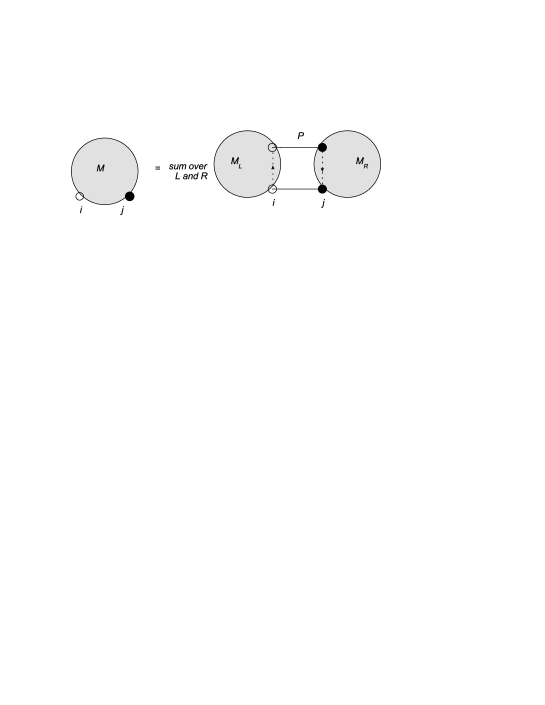
Figure 1: Hodges diagram for the BCFW relations.

Figure 2: Some ingredients in Hodges diagrams.

In this paper we will compute the amplitudes using the BCFW relation in super-ambitwistor space [12]:

$$M({\cal W}_{i},{\cal Z}_{j})=\sum_{L,R}\int\large[D^{3|4}{\cal W}_{P}D^{3|4}{\cal Z}_{P}\large]_{{\cal W}_{i},{\cal Z}_{j}}M_{L}({\cal W}_{i};{\cal W}_{P})M_{R}({\cal Z}_{j};{\cal Z}_{P}).$$ (8)

Here the projective measure is defined as:

$$\large[D^{3|4}{\cal W}_{P}D^{3|4}{\cal Z}_{P}\large]_{{\cal W}_{i},{\cal Z}_{j}} = D^{3|4}{\cal W}_{P}D^{3|4}{\cal Z}_{P}\,{\rm sgn}({\cal W}_{i}\cdot{\cal Z}_{j}){\rm sgn}({\cal W}_{P}\cdot{\cal Z}_{P})$$ (9)

$$\times {\rm sgn}({\cal W}_{i}I{\cal W}_{P}){\rm sgn}({\cal Z}_{P}I{\cal Z}_{j})$$

The projective measure can be de-projectivized as:

$$M({\cal W}_{i},{\cal Z}_{j}) = \sum_{L,R}\int d^{4|4}{\cal W}d^{4|4}{\cal Z}{\rm sgn}({\cal W}_{i}\cdot{\cal Z}_{j}){\rm sgn}({\cal W}\cdot{\cal Z})\exp[i{\cal W}_{i}I{\cal W}]$$ (10)

$$\exp[i{\cal Z}I{\cal Z}_{j}]M_{L}({\cal W}_{i},{\cal W})M_{R}({\cal Z}_{j},{\cal Z}).$$

In [12], the above relation is presented using Hodges diagram as in Fig. 1. Some ingredients in Hodges diagrams are listed in Fig. 2. Notice that we add an arrow to the dash line comparing with [12] since ${\rm sgn}({\cal W}_{i}I{\cal W}_{j})$ is anti-symmetric. We also add an arrow to the wavy line. The reason is that, as discussed in [12], the factor $\exp[i{\cal Z}\cdot{\cal W}]$ usually appears with integration over ${\cal Z}$ or ${\cal W}$ to represent a super-twistor transformation (a super-Fourier transformation). We use the arrow toward ${\cal Z}$ (or ${\cal W}$) to represent integration over ${\cal Z}$ (or ${\cal W}$). We find that this is quite useful to make things clear in the complicated diagrams we will meet later.

3 Computations of split helicity amplitudes in ambitwistor space

3.1 General discussions on split helicity amplitudes

Now we begin our study of the split helicity amplitude $M(1,+;\cdots,q,+;(q+1),-;\cdots,n,-)$ in ambitwistor space. We first make the following choice between $W$ and $Z$ for the external gluons:

$$M(W_{1},+;\cdots,W_{q},+;Z_{q+1},-;\cdots,Z_{n},-),$$ (11)

since with this choice the amplitudes have weight zero with respect to independent rescalings of each $W$ or $Z$. Notice that at tree level, the pure gluonic amplitudes in pure Yang-Mills theory are the same as the ones in ${\cal N}=4$ super Yang-Mills theory. Now we lift these amplitudes to the super-amplitudes $M({\cal W}_{1},\cdots,{\cal W}_{q},{\cal Z}_{q+1},\cdots,{\cal Z}_{n})$. The split helicity gluonic amplitudes can be obtained from the super-amplitudes through the following Grassman integral:

$$M(W_{1},+;\cdots,W_{q},+;Z_{q+1},-;\cdots,Z_{n},-)=\int d^{4}\tilde{\eta}_{1}\cdots d^{4}\tilde{\eta}_{q}d^{4}\eta_{q+1}\cdots d^{4}\eta_{n}$$

$$\qquad\qquad\qquad\qquad\qquad\prod_{j=1}^{q}(\tilde{\eta}_{j})^{4}\prod_{j=q+1}^{n}(\eta_{j})^{4}M({\cal W}_{1},\cdots,{\cal W}_{q},{\cal Z}_{q+1},\cdots,{\cal Z}_{n}).$$ (12)

To compute the split helicity amplitudes, we do not need to completely compute the superamplitudes. Instead we pick out the Hodges diagrams contributing to these special gluonic amplitudes, by doing Grassman integrals. This play a very crucial role in our computations.

For the superamplitudes $M({\cal W}_{1},\cdots,{\cal W}_{q},{\cal Z}_{q+1},\cdots,{\cal Z}_{n})$, choosing $i$ and $j$ in eq. (8) to be $1$ and $n$ respectively, the BCFW relation now becomes:

$$M({\cal W}_{1},\cdots,{\cal W}_{q},{\cal Z}_{q+1},\cdots,{\cal Z}_{n})=\int\large[D^{3|4}{\cal W}_{P}D^{3|4}{\cal Z}_{P}\large]_{{\cal W}_{1},{\cal Z}_{n}}$$

$$\qquad\qquad(\sum_{i=2}^{q}M_{L}({\cal W}_{1},\cdots,{\cal W}_{i},{\cal W}_{P})M_{R}({\cal Z}_{P},{\cal W}_{i+1},\cdots,{\cal W}_{q},{\cal Z}_{q+1},\cdots,{\cal Z}_{n})$$

$$\qquad\qquad+\sum_{i=q+1}^{n-2}M_{L}({\cal W}_{1},\cdots,{\cal W}_{q},{\cal Z}_{q+1}\cdots,{\cal Z}_{i},{\cal W}_{P})M_{R}({\cal Z}_{P},{\cal Z}_{i+1},\cdots,{\cal Z}_{n})).$$ (13)

Using eq. (12) and eq. (13), we get:

$$M(W_{1},+;\cdots,W_{q},+;Z_{q+1},-;\cdots,Z_{n},-)=\int d^{4}\tilde{\eta}_{1}d^{4}\eta_{n}(\tilde{\eta}_{1})^{4}(\eta_{n})^{4}$$

$$\qquad\qquad\int\large[D^{3|4}{\cal W}_{P}D^{3|4}{\cal Z}_{P}\large]_{{\cal W}_{1},{\cal Z}_{n}}\left(\sum_{i=2}^{q}\int\prod_{j=2}^{i}d^{4}\tilde{\eta}_{j}(\tilde{\eta}_{j})^{4}M_{L}({\cal W}_{1},\cdots,{\cal W}_{i},{\cal W}_{P})\right.$$

$$\qquad\qquad\int\prod_{j=i+1}^{q}d^{4}\tilde{\eta}_{j}(\tilde{\eta}_{j})^{4}\prod_{j=q+1}^{n-1}d^{4}\eta_{j}(\eta_{j})^{4}M_{R}({\cal Z}_{P},{\cal W}_{i+1},\cdots,{\cal W}_{q},{\cal Z}_{q+1},\cdots,{\cal Z}_{n})$$

$$\qquad\qquad+\sum_{i=q+1}^{n-2}\int\prod_{j=2}^{q}d^{4}\tilde{\eta}_{j}(\tilde{\eta}_{j})^{4}\prod_{j=q+1}^{i}d^{4}\eta_{j}\eta_{j}^{4}M_{L}({\cal W}_{1},\cdots,{\cal W}_{q},{\cal Z}_{q+1},\cdots,{\cal Z}_{i},{\cal W}_{P})$$

$$\qquad\qquad\left.\int\prod_{j=i+1}^{n-1}d^{4}\eta_{j}\eta_{j}^{4}M_{R}({\cal Z}_{P},{\cal Z}_{i+1},\cdots,{\cal Z}_{n})\right).$$ (14)

Since we want to use these Grassman integrals to pick out the needed Hodges diagrams, we also need to deal with the integration over $\tilde{\eta}_{1}$ and $\eta_{n}$ . To do this, let us consider the more general integral:

$$\int d^{4}\tilde{\eta}_{1}d^{4}\eta_{n}\tilde{\eta}_{1}^{4}\eta_{n}^{4}\int\large[D^{3|4}{\cal W}_{P}D^{3|4}{\cal Z}_{P}\large]_{{\cal W}_{1},{\cal Z}_{n}}F({\cal W}_{P},{\cal Z}_{P}),$$ (15)

where $F({\cal W},{\cal Z})$ is a function of weight zero. As before, we can de-projectivize the projective measure:

$$\int d^{4}\tilde{\eta}_{1}d^{4}\eta_{n}\tilde{\eta}_{1}^{4}\eta_{n}^{4}\int\large[D^{3|4}{\cal W}_{P}D^{3|4}{\cal Z}_{P}\large]_{{\cal W}_{1},{\cal Z}_{n}}F({\cal W}_{P},{\cal Z}_{P})$$

$$\qquad\qquad=\int d^{4}\tilde{\eta}_{1}d^{4}\eta_{n}\tilde{\eta}_{1}^{4}\eta_{n}^{4}\int D^{4|4}{\cal W}D^{4|4}{\cal Z}{\rm{\rm sgn}}({\cal W}_{1}\cdot{\cal Z}_{n})$$

$$\qquad\qquad\qquad{\rm sgn}({\cal W}\cdot{\cal Z})\exp(i{\cal W}_{1}I{\cal W})\exp(i{\cal Z}I{\cal Z}_{n})F({\cal W},{\cal Z}).$$ (16)

By using

$${\rm sgn}(x)=\int\frac{da}{a}\exp(iax),$$ (17)

we get

$$\int d^{4}\tilde{\eta}_{1}d^{4}\eta_{n}\tilde{\eta}_{1}^{4}\eta_{n}^{4}\int\large[D^{3|4}{\cal W}_{P}D^{3|4}{\cal Z}_{P}\large]_{{\cal W}_{1},{\cal Z}_{n}}F({\cal W}_{P},{\cal Z}_{P})$$

$$\qquad\qquad=\int D^{4|4}{\cal W}D^{4|4}{\cal Z}({\rm sgn}({\cal W}_{1}\cdot{\cal Z}_{n}){\rm sgn}({\cal W}\cdot{\cal Z})\exp(i{\cal W}_{1}I{\cal W})\exp(i{\cal Z}I{\cal Z}_{n})$$

$$\qquad\qquad\qquad F({\cal W},{\cal Z}))|_{{\cal W}_{1}\to W_{1},{\cal Z}_{n}\to Z_{n}}.$$ (18)

So in eq. (13), performing the integration:

$$\int d^{4}\tilde{\eta}_{1}d^{4}\eta_{n}\tilde{\eta}_{1}^{4}\eta_{n}^{4}$$ (19)

is just performing the replacement:

$${\cal W}_{1}\to W_{1},{\cal Z}_{n}\to Z_{n}$$ (20)

as usual, and the projective measure will not affect this.

Now consider $M_{L}$ in the first sum in eq. (13), it appears in the following way:

$$\int\prod_{j=2}^{i}d^{4}\tilde{\eta}_{j}\tilde{\eta}_{j}^{4}M({\cal W}_{1},\cdots,{\cal W}_{i},{\cal W}_{P})|_{{\cal W}_{1}\to W_{1}}=M(W_{1},+,\cdots,W_{i},+,{\cal W}_{P})$$ (21)

By writing this superamplitudes as linear combination of amplitudes, we can see that the above result vanishes when $i>2$. So only the term with $i=2$ contributes to the first sum of eq. (13). Similarly only term with $i=n-2$ in the second sum contributes. As a result for $n>4$, only two terms have nonvanishing contribution, while for $n=4$ only one term contributes. Use this we can throw away many Hodges diagrams which will not contribute to the split helicity amplitudes. This simplifies the computations significantly.

Two other useful relations are:

$$\int d^{4}\tilde{\eta}_{1}d^{4}\tilde{\eta}_{2}\tilde{\eta}_{1}^{4}\tilde{\eta}^{4}_{2}M({\cal W}_{1},{\cal W}_{2},{\cal W}) = M^{++-}(W_{1},W_{2},W)\tilde{\eta}^{4}$$ (22)

$$= \int d^{4}\tilde{\eta}_{1}d^{4}\tilde{\eta}_{2}\tilde{\eta}^{4}_{1}\tilde{\eta}^{4}_{2}M^{+}({\cal W}_{1},{\cal W}_{2},{\cal W}),$$

$$\int d^{4}\eta_{n-1}d^{4}\eta_{n}\eta^{4}_{n-1}\eta^{4}_{n}M({\cal Z}_{n-1},{\cal Z}_{n},{\cal Z}) = M^{--+}(Z_{1},Z_{2},Z)\eta^{4}$$ (23)

$$= \int d^{4}\eta_{n-1}d^{4}\eta_{n}\eta^{4}_{n-1}\eta^{4}_{n}M^{-}({\cal Z}_{n-1},{\cal Z}_{n},{\cal Z}),$$

where

$$M^{+}({\cal W}_{1},{\cal W}_{2},{\cal W})=\int d^{4|4}{\cal Z}e^{i{\cal W}\cdot{\cal Z}}{\rm sgn}({\cal W}_{1}I{\cal W}_{2}){\rm sgn}({\cal W}_{1}\cdot{\cal Z}){\rm sgn}({\cal W}_{2}\cdot{\cal Z}),$$ (24)

$$M^{-}({\cal Z}_{n-1},{\cal Z}_{n},{\cal Z})=\int d^{4|4}{\cal W}e^{i{\cal Z}\cdot{\cal W}}{\rm sgn}({\cal Z}_{n-1}I{\cal Z}_{n}){\rm sgn}({\cal Z}_{n-1}\cdot{\cal W}){\rm sgn}({\cal Z}_{n}\cdot{\cal W}),$$ (25)

are given in [12]. The first lines of eq. (22) can be understood as follows: the integration over $\tilde{\eta}$’s fix the helicity of ${\cal W}_{1}$ and ${\cal W}_{2}$, then the helicity of ${\cal W}$ is fixed to be $-1$ for the amplitude to be nonzero. The fact that, in eq. (24) (eq. (25)), only $M^{+}$ ($M^{-}$) contributes can also be obtained from the “vanishing” identity in [12].

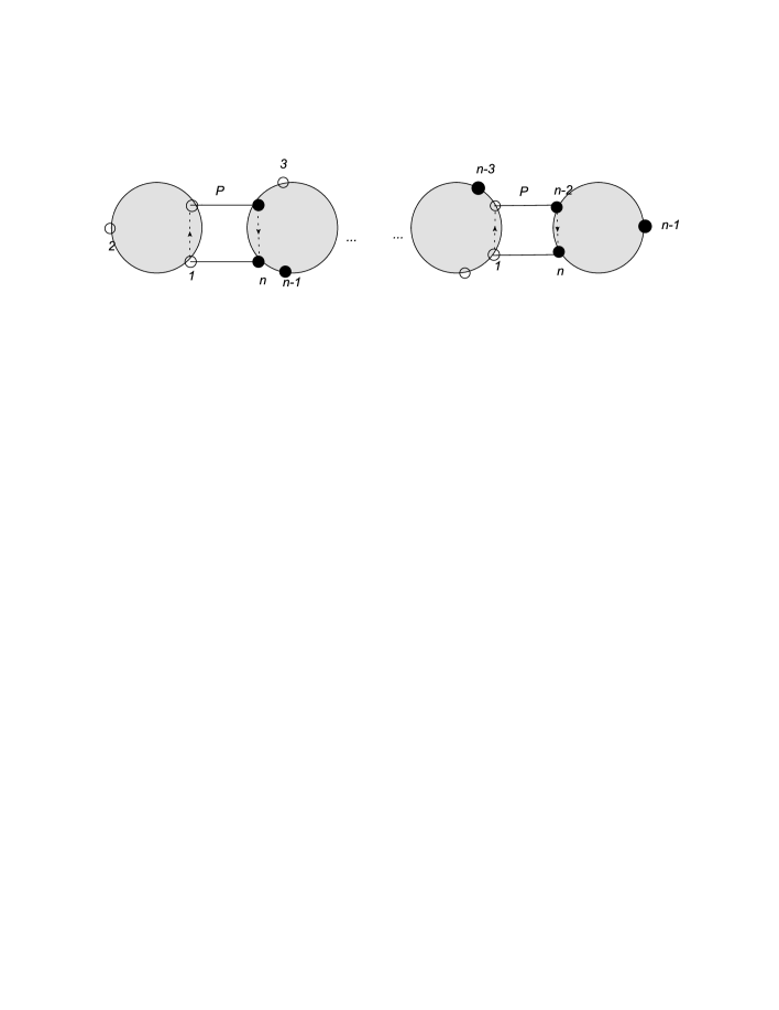
Figure 3: The contributing Hodges diagrams.

The above discussions lead to the following results for the amplitudes with $n>4$ gluons:

$$M(W_{1},+;\cdots,W_{q},+;Z_{q+1},-;\cdots,Z_{n},-)=\int d^{4}\tilde{\eta}_{1}d^{4}\eta_{n}(\tilde{\eta}_{1})^{4}(\eta_{n})^{4}$$

$$\qquad\qquad\int\large[D^{3|4}{\cal W}_{P}D^{3|4}{\cal Z}_{P}\large]_{{\cal W}_{1},{\cal Z}_{n}}\left(\int d^{4}\tilde{\eta}_{2}(\tilde{\eta}_{2})^{4}M^{+}({\cal W}_{1},{\cal W}_{2},{\cal W}_{P})\right.$$

$$\qquad\qquad\int\prod_{j=i+1}^{q}d^{4}\tilde{\eta}_{j}(\tilde{\eta}_{j})^{4}\prod_{j=q+1}^{n-1}d^{4}\eta_{j}(\eta_{j})^{4}M_{R}({\cal Z}_{P},{\cal W}_{i+1},\cdots,{\cal W}_{q},{\cal Z}_{q+1},\cdots,{\cal Z}_{n})+$$

$$\qquad\qquad\int\prod_{j=2}^{q}d^{4}\tilde{\eta}_{j}(\tilde{\eta}_{j})^{4}\prod_{j=q+1}^{n-2}d^{4}\eta_{j}\eta_{j}^{4}M_{L}({\cal W}_{1},\cdots,{\cal W}_{q},{\cal Z}_{q+1},\cdots,{\cal Z}_{n-2},{\cal W}_{P})$$

$$\qquad\qquad\left.\int d^{4}\eta_{n-1}\eta_{n-1}^{4}M^{-}({\cal Z}_{P},{\cal Z}_{n-1},{\cal Z}_{n})\right).$$ (26)

The result can be expressed as in Fig. 3.

The BCFW relation in the super-twistor space treat the whole ${\cal N}=4$ multiplet once at a time by using the on-shell ${\cal N}=4$ superspace. As we can see from the above, fixing the helicities of the external gluon fixes the helicities of some internal particles in some Hodges diagrams. This in turn fixes some helicities of other internal particles. The reason is that as the BCFW relation for gluonic amplitudes in momentum space, the helicity of ${\cal W}_{P}$ and ${\cal Z}_{P}$ should be opposite for each term in the expansion of the superamplitudes in the right-hand-side of eq. (8). To see this, using eqs. (7, 10, 17), we can pick out the integral over $\eta$ and $\tilde{\eta}$ in $M$,

$$\int d^{4}\eta d^{4}\tilde{\eta}\exp[ia\eta\cdot\tilde{\eta}]M_{L}(\tilde{\eta})M_{R}(\eta).$$ (27)

If we consider the terms in $M_{L}$ whose ${\cal W}_{P}$ has helicity $+1$ ($-1$), then these terms will have no $\tilde{\eta}$’s (four $\tilde{\eta}$’s). From the above equation, we can see that the terms in $M_{R}$ with no $\eta$’s (four $\eta$’s) are picked out, which means that the helicity of ${\cal Z}_{P}$ have to be $-1$ ($+1$). (This result is also valid if we exchange (${\cal W}_{P}$, $\tilde{\eta}$) and (${\cal Z}_{P}$, $\eta$).) We have seen that in the first term of eq. (26), the helicity of ${\cal W}_{P}$ is fixed by eq. (22) to be $-1$. Then the helicity of ${\cal Z}_{P}$ in this term is fixed to be $+1$, the same as the helicity of ${\cal W}_{2}$. This guarantees that we can treat the remaining $M_{R}$ as a split helicity amplitude similar to the one we begin with and we can still throw away many Hodges diagrams when we compute it using BCFW rules as the first step. We have similar results for the second term in eq. (26).

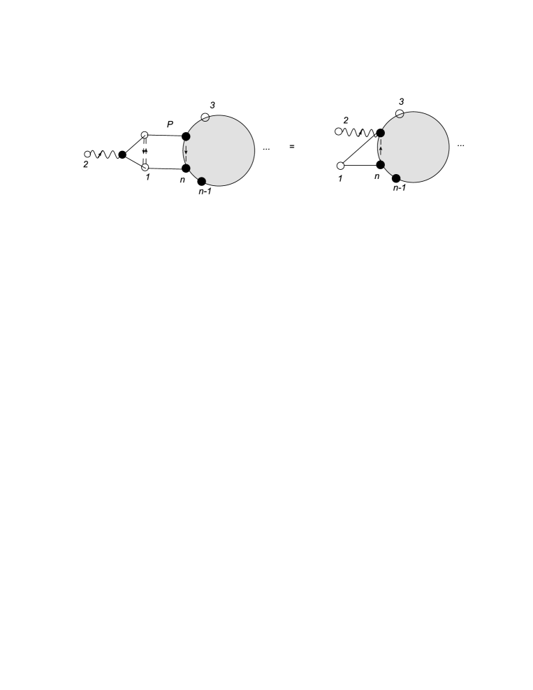
Figure 4: Simplifying the left graph in Fig. 3 using various identities.

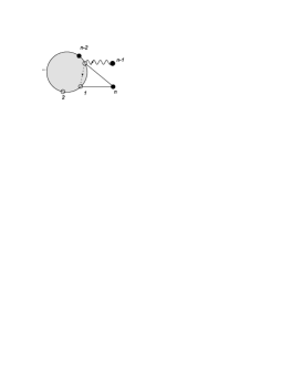
Figure 5: Simplifying the right graph in Fig. 3 using various identities.

Now we can use the Hodges diagram for three gluon amplitudes $M^{\pm}_{sym}$, ${\rm sgn}^{2}=1$ and “scrunch” identity in [12] to simplify the graphs in Fig. 3. The first graph is simplified as Fig. 4, while the second graph is simplified to be Fig. 5. We can think Fig. 4 and Fig. 5 as the simplified recursion relations in this special case.

3.2 A special case: split MHV amplitudes

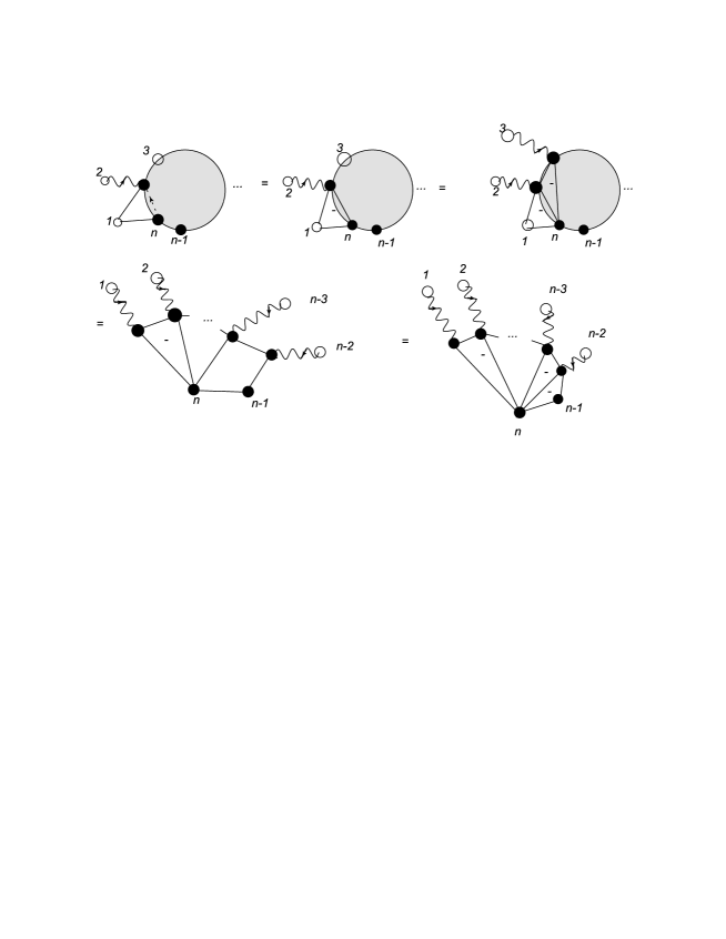
Figure 6: The split MHV amplitudes.

Figure 7: The triangles.

Let us now have a close look at the split MHV amplitudes because they are the simplest and later we will find that they will be one of the building blocks of the general split helicity amplitudes. Let us consider the amplitudes

$$M(W_{1},+;\cdots,W_{n-2},+;Z_{n-1},-;Z_{n},-).$$ (28)

Using the arguments in previous section, we can perform the calculations as in Fig. 6. We use the triangles with signs to represent $-M^{\pm}_{3}$ (Fig. 7), as in [20, 21]. Notice that in this special case, at every step, we only have one diagram since the other one vanishes due to the vanishing of the subamplitude $M^{+\cdots+-}$. Here we have also used the results for four-gluon MHV amplitudes in [12].

Figure 8: The MHV domain.

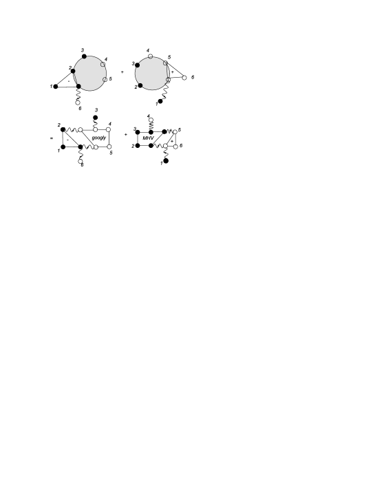
Figure 9: A NMHV six-gluon amplitude.

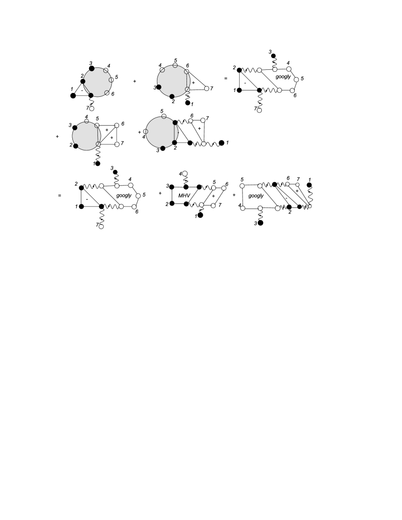
Figure 10: A NNMHV seven-gluon amplitude.

From this result, we can see that the more natural choice of ${\cal W}$’s and ${\cal Z}$’s is to choose ${\cal Z}$’s for all of the external gluons. We can draw the diagram as in Fig. 8. We find that the triangles are combined into a MHV-domains [20, 21]. Similarly we can get the $\overline{MHV}$(googly)-domain, by changing all ${\cal Z}$’s into ${\cal W}$’s and all black nods into white nods.

3.3 Two non-MHV examples

Figure 11: The diagrams for generic split helicity amplitudes: part I.

Figure 12: The diagrams for generic split helicity amplitudes: part II.

The results for MHV and $\overline{MHV}$ amplitudes indicates that for split helicity amplitudes a better choice is to choose ${\cal Z}$’s for the positive helicity gluons and ${\cal W}$’s for the negative helicity gluons. Let us make this choice and compute, as examples, the six-gluon NMHV amplitude $A_{6}(+++---)$ and seven-gluon NNMHV (while $\overline{NMHV}$) amplitude $A_{7}(+++----)$. The diagrammatic representation of the computations and the results are put in Fig. 9 and Fig. 10 respectively. Notice that in Fig. 10, we meet another situation that some triangles with $+$ signs are combined into a domain. The helicities of the external gluons in this domain is neither $MHV$ or $\overline{MHV}$. we call this domain type II$+$ domain. Similarly we will meet type II$-$ domain made up of triangles with $-$ signs in the diagrams for other amplitudes.

Figure 13: The ziazag diagrams.

3.4 General Results

Now we can draw the diagrams for the generic split helicity amplitudes as in Fig 11 and Fig. 12. In these diagrams, all domains besides the MHV or googly domains are type II domains. We just use $+$ or $-$ to denote type II$+$ or type II$-$ domains in these diagrams. There is exactly one external gluon with positive (negative) helicity in type II$+$ (type II$-$) domains . In our diagrams, all of the nods for the gluons are choose to be white (black) for the type II$+$ (type II$-$) domains. We can simply express every diagram using zigzag diagrams (Fig. 13). Totally we have four types of zigzag diagrams:

$$1=i_{0}<i_{1}<i_{2}<\cdots<i_{m}=q-1,n>j_{1}>j_{2}>\cdots>j_{m}>q+1,$$ (29)

$$1=i_{0}<i_{1}<i_{2}<\cdots<i_{m-1}<q,n>j_{1}>j_{2}>\cdots>j_{m}=q+2,$$ (30)

$$1<i_{1}<i_{2}<\cdots<i_{m}<q,n=j_{0}>j_{1}>\cdots>j_{m}=q+2,$$ (31)

$$1<i_{1}<i_{2}<\cdots<i_{m}=q-1,n=j_{0}>j_{1}>\cdots>j_{m}>q+1.$$ (32)

The final result for the split helicity gluonic amplitudes we want to compute is:

$$M^{+\cdots+-\cdots-}(Z_{1},\cdots,Z_{q},W_{q+1},\cdots,W_{n})=\int\prod_{i=1}^{q}d^{4}\eta_{i}\prod_{j=q+1}^{n}d^{4}\tilde{\eta}_{j}$$

$$\qquad\qquad\qquad\qquad\tilde{\cal M}({\cal Z}_{1},\cdots,{\cal Z}_{q},{\cal W}_{q+1},\cdots,{\cal W}_{n}),$$ (33)

where

$$\tilde{\cal M}=\sum_{I}\tilde{\cal M}_{I}+\sum_{II}\tilde{\cal M}_{II}+\sum_{III}\tilde{\cal M}_{III}+\sum_{IV}\tilde{\cal M}_{IV}.$$ (34)

The summation is over the zigzags and

$$\tilde{\cal M}_{I}=\int d^{4|4}{\cal W}_{1}\exp[i{\cal W}_{1}\cdot{\cal Z}_{1}]\tilde{\cal M}^{+}({\cal W}_{1};{\cal W}_{j_{1}},\cdots,{\cal W}_{n})$$

$$\qquad\qquad\int d^{4|4}{\cal Z}_{j_{1}}\exp[i{\cal Z}_{j_{1}}\cdot{\cal W}_{j_{1}}]\int d^{4|4}{\cal Z}_{1}^{\prime}\exp[i{\cal Z}_{1}^{\prime}\cdot{\cal W}_{1}]\tilde{\cal M}^{-}({\cal Z}_{j_{1}};{\cal Z}_{1}^{\prime},\cdots,{\cal Z}_{i_{1}})$$

$$\qquad\qquad\int d^{4|4}{\cal W}_{j_{1}}^{\prime}\exp[i{\cal W}_{j_{1}}^{\prime}\cdot{\cal Z}_{j_{1}}]\int d^{4|4}{\cal W}_{i_{1}}\exp[i{\cal W}_{i_{1}}\cdot{\cal Z}_{i_{1}}]\tilde{\cal M}^{+}({\cal W}_{i_{1}};{\cal W}_{j_{2}},\cdots,{\cal W}_{j_{1}}^{\prime})$$

$$\qquad\qquad\cdots\int d^{4|4}{\cal Z}_{i_{m-1}}^{\prime}\exp[i{\cal Z}_{i_{m-1}}\cdot{\cal W}_{i_{m-1}}]\int d^{4|4}{\cal Z}_{q+2}\exp[i{\cal Z}_{q+2}\cdot{\cal W}_{q+2}]$$

$$\qquad\qquad\int d^{4|4}{\cal Z}_{q+1}\exp[i{\cal Z}_{q+1}\cdot{\cal W}_{q+1}]\tilde{\cal M}_{MHV}({\cal Z}_{q+1},{\cal Z}_{q+2};{\cal Z}_{i_{m-1}}^{\prime},\cdots,{\cal Z}_{q}),$$ (35)

$$\tilde{\cal M}_{II}=\int d^{4|4}{\cal W}_{1}\exp[i{\cal W}_{1}\cdot{\cal Z}_{1}]\tilde{\cal M}^{+}({\cal W}_{1};{\cal W}_{j_{1}},\cdots,{\cal W}_{n})$$

$$\qquad\qquad\cdots\int d^{4|4}{\cal W}_{j_{m}}^{\prime}\exp[i{\cal W}_{j_{m}}^{\prime}\cdot{\cal Z}_{j_{m}}]\int d^{4|4}{\cal W}_{q-1}\exp[i{\cal W}_{q-1}\cdot{\cal Z}_{q-1}]$$

$$\qquad\qquad\int d^{4|4}{\cal W}_{q}\exp[i{\cal W}_{q}\cdot{\cal Z}_{q}]\tilde{\cal M}_{\overline{MHV}}({\cal W}_{q-1},{\cal W}_{q};{\cal W}_{q+1},\cdots,{\cal W}_{j_{m-1}}^{\prime}),$$ (36)

$$\tilde{\cal M}_{III}=\int d^{4|4}{\cal Z}_{n}\exp[i{\cal Z}_{n}\cdot{\cal W}_{n}]\tilde{\cal M}^{-}({\cal Z}_{n};{\cal Z}_{1},\cdots,{\cal Z}_{i_{1}})$$

$$\qquad\qquad\int d^{4|4}{\cal W}_{n}^{\prime}\exp[i{\cal W}_{n}^{\prime}\cdot{\cal Z}_{n}]\int d^{4|4}{\cal W}_{i_{1}}\exp[i{\cal W}_{i_{1}}\cdot{\cal Z}_{i_{1}}]\tilde{\cal M}^{+}({\cal W}_{i_{1}};{\cal W}_{j_{1}},\cdots,{\cal W}_{n})$$

$$\qquad\qquad\cdots\int d^{4|4}{\cal Z}_{i_{m}}^{\prime}\exp[i{\cal Z}_{i_{m}}^{\prime}\cdot{\cal W}_{i_{m}}]\int d^{4|4}{\cal Z}_{q+2}\exp[i{\cal Z}_{q+2}\cdot{\cal W}_{q+2}]$$

$$\qquad\qquad\int d^{4|4}{\cal Z}_{q+1}\exp[i{\cal Z}_{q+1}\cdot{\cal W}_{q+1}]\tilde{\cal M}_{MHV}({\cal Z}_{q+1},{\cal Z}_{q+2};{\cal Z}_{i_{m}}^{\prime},\cdots,{\cal Z}_{q}),$$ (37)

$$\tilde{\cal M}_{IV}=\int d^{4|4}{\cal Z}_{n}\exp[i{\cal Z}_{n}\cdot{\cal W}_{n}]\tilde{\cal M}^{-}({\cal Z}_{n};{\cal Z}_{1},\cdots,{\cal Z}_{i_{1}})$$

$$\qquad\qquad\cdots\int d^{4|4}{\cal W}_{j_{m-1}}^{\prime}\exp[i{\cal W}_{j_{m-1}}^{\prime}\cdot{\cal Z}_{j_{m-1}}]\int d^{4|4}{\cal Z}_{q-1}\exp[i{\cal Z}_{q-1}\cdot{\cal W}_{q-1}]$$

$$\qquad\qquad\int d^{4|4}{\cal W}_{q}\exp[i{\cal W}_{q}\cdot{\cal Z}_{q}]\tilde{\cal M}_{\overline{MHV}}({\cal W}_{q-1},{\cal W}_{q};{\cal W}_{q+1}\cdots,{\cal W}_{j_{m-1}}^{\prime}).$$ (38)

Here the expressions for the type II domain are:

$$\tilde{\cal M}^{+}({\cal W}_{j};{\cal W}_{i},{\cal W}_{i+1},\cdots,{\cal W}_{l}) = (-1)^{l-i}\prod_{k=i}^{l-1}\tilde{\cal M}^{+}({\cal W}_{j},{\cal W}_{k},{\cal W}_{k+1}),$$ (39)

$$\tilde{\cal M}^{-}({\cal Z}_{j};{\cal Z}_{i},{\cal Z}_{i+1},\cdots,{\cal Z}_{l}) = (-1)^{l-i}\prod_{k=i}^{l-1}\tilde{\cal M}^{-}({\cal Z}_{j},{\cal Z}_{k},{\cal Z}_{k+1}).$$ (40)

The expressions for MHV and $\overline{MHV}$ domains are:

$$\tilde{\cal M}_{MHV}({\cal Z}_{q+1},{\cal Z}_{q+2};{\cal Z}_{i_{m}},\cdots,{\cal Z}_{q}) = (-1)^{q-i_{m}+1}\prod_{k=i_{m}}^{q-1}M^{-}({\cal Z}_{q+1},{\cal Z}_{k},{\cal Z}_{k+1})$$ (41)

$$\times M^{-}({\cal Z}_{q+1},{\cal Z}_{q+2},{\cal Z}_{i_{m}}),$$

$$\tilde{\cal M}_{\overline{MHV}}({\cal W}_{q-1},{\cal W}_{q};{\cal W}_{q+1},\cdots,{\cal W}_{j_{m}}) = (-1)^{j_{m}-q}\prod_{i=q+1}^{j_{m}-1}M^{+}({\cal W}_{q-1},{\cal W}_{q},{\cal W}_{j_{m}})$$ (42)

$$\times M^{+}({\cal W}_{q-1},{\cal W}_{q},{\cal W}_{j_{m}}),$$

where $M^{-}({\cal Z}_{1},{\cal Z}_{2},{\cal Z}_{3}),M^{+}({\cal W}_{1},{\cal W}_{2},{\cal W}_{3})$ are given in eqs. (24, 25). The fact that all the amplitudes are composed of the domains shows that all tree-level split helicity amplitudes are triangulable.

We can see from these result that the most natural choices of ${\cal W}$’s and ${\cal Z}$’s for $1$, $q$, $q+1$, $n$ are different in different terms. Similar phenomenon appears in the amplitudes for gravitons in [12].

By using the ’triangle identity’ in [12], we can rewrite eqs. (24, 25) in a suitable way and perform all of the Grassman integrations to get:

$$M(Z_{1},+;\cdots;Z_{q},+;W_{q+1},-;\cdots;W_{n},-)=\sum_{I}M_{I}+\sum_{II}M_{II}+\sum_{III}M_{III}+\sum_{IV}M_{IV}.$$ (43)

Here the summation is still over the zigzags. Now

$$M_{I}=\int d^{4}W_{1}\exp[iW_{1}\cdot Z_{1}]\tilde{\cal M}^{+}(W_{1},+;W_{j_{1}},-;\cdots;W_{n},-)$$

$$\qquad\qquad\int d^{4}Z_{j_{1}}\exp[iZ_{j_{1}}\cdot W_{j_{1}}]\int d^{4}Z_{1}^{\prime}\exp[iZ_{1}^{\prime}\cdot W_{1}]\tilde{\cal M}^{-}(Z_{j_{1}},-;Z_{1}^{\prime},+;\cdots;Z_{i_{1}},+)$$

$$\qquad\qquad\int d^{4}W_{j_{1}}^{\prime}\exp[iW_{j_{1}}^{\prime}\cdot Z_{j_{1}}]\int d^{4}W_{i_{1}}\exp[iW_{i_{1}}\cdot Z_{i_{1}}]\tilde{\cal M}^{+}(W_{i_{1}},+;W_{j_{2}},-;\cdots;W_{j_{1}}^{\prime},-)$$

$$\qquad\qquad\cdots\int d^{4}Z_{i_{m-1}}^{\prime}\exp[iZ_{i_{m-1}}\cdot W_{i_{m-1}}]\int d^{4}Z_{q+2}\exp[iZ_{q+2}\cdot W_{q+2}]$$

$$\qquad\qquad\int d^{4}Z_{q+1}\exp[iZ_{q+1}\cdot W_{q+1}]\tilde{\cal M}_{MHV}(Z_{i_{m-1}}^{\prime},+;\cdots;Z_{q},+;Z_{q+1},-;Z_{q+2},-),$$ (44)

$$M_{II}=\int d^{4}W_{1}\exp[iW_{1}\cdot Z_{1}]\tilde{\cal M}^{+}(W_{1},+;W_{j_{1}},-;\cdots;W_{n},-)$$

$$\qquad\qquad\cdots\int d^{4}W_{j_{m}}^{\prime}\exp[iW_{j_{m}}^{\prime}\cdot Z_{j_{m}}]\int d^{4}W_{q-1}\exp[iW_{q-1}\cdot Z_{q-1}]$$

$$\qquad\qquad\int d^{4}W_{q}\exp[iW_{q}\cdot Z_{q}]\tilde{\cal M}_{\overline{MHV}}(W_{q-1},+;W_{q},+;W_{q+1},-;\cdots;W_{j_{m-1}}^{\prime},-),$$ (45)

$$M_{III}=\int d^{4}Z_{n}\exp[iZ_{n}\cdot W_{n}]\tilde{\cal M}^{-}(Z_{n},-;Z_{1},+;\cdots,Z_{i_{1}},+)$$

$$\qquad\qquad\int d^{4}W_{n}^{\prime}\exp[iW_{n}^{\prime}\cdot Z_{n}]\int d^{4}W_{i_{1}}\exp[iW_{i_{1}}\cdot Z_{i_{1}}]\tilde{\cal M}^{+}(W_{i_{1}},+;W_{j_{1}},-;\cdots,W_{n},-)$$

$$\qquad\qquad\cdots\int d^{4}Z_{i_{m}}^{\prime}\exp[iZ_{i_{m}}^{\prime}\cdot W_{i_{m}}]\int d^{4}Z_{q+2}\exp[iZ_{q+2}\cdot W_{q+2}]$$

$$\qquad\qquad\int d^{4}Z_{q+1}\exp[iZ_{q+1}\cdot W_{q+1}]\tilde{\cal M}_{MHV}(Z_{i_{m}}^{\prime},+;\cdots;Z_{q},+;Z_{q+1},-;Z_{q+2},-),$$ (46)

$$\tilde{\cal M}_{IV}=\int d^{4}Z_{n}\exp[iZ_{n}\cdot W_{n}]\tilde{\cal M}^{-}(Z_{n},-;Z_{1},+;\cdots,Z_{i_{1}},+)$$

$$\qquad\qquad\cdots\int d^{4}W_{j_{m-1}}^{\prime}\exp[iW_{j_{m-1}}^{\prime}\cdot Z_{j_{m-1}}]\int d^{4}Z_{q-1}\exp[iZ_{q-1}\cdot W_{q-1}]$$

$$\qquad\qquad\int d^{4}W_{q}\exp[iW_{q}\cdot Z_{q}]\tilde{\cal M}_{\overline{MHV}}(W_{q-1},+;W_{q},+;W_{q+1},-;\cdots;W_{j_{m-1}}^{\prime},-).$$ (47)

The express for the type II domains and MHV/$\overline{MHV}$ domains are:

$$\tilde{\cal M}^{-}(Z_{j},-;Z_{i},+;Z_{i+1},+;\cdots;Z_{l},+)=(-1)^{l-i}\prod_{k=i}^{l-1}\tilde{\cal M}^{-}(Z_{j},Z_{k},Z_{k+1})$$ (48)

$$\tilde{\cal M}^{+}(W_{j},+;W_{i},-;W_{i+1},-;\cdots;W_{l},-)=(-1)^{l-i}\prod_{k=i}^{l-1}\tilde{\cal M}^{+}(W_{j},W_{k},W_{k+1}),$$ (49)

$$\tilde{\cal M}_{MHV}(Z_{i_{m}},+;\cdots;Z_{q},+;Z_{q+1},-;Z_{q+2},-)=(-1)^{q-i_{m}}\tilde{\cal M}^{-}(Z_{q-1},Z_{q+1},Z_{q+2})$$

$$\tilde{\cal M}^{-}(Z_{q},Z_{q-1},Z_{q+1})\prod_{l=i_{m}}^{q-2}\tilde{\cal M}^{-}(Z_{l},Z_{l+1},Z_{q+2}),$$ (50)

$$\tilde{\cal M}_{\overline{MHV}}(W_{q-1},+;W_{q},+;W_{q+1},-;\cdots;W_{j_{m}},-)=(-1)^{j_{m}-q+1}\tilde{\cal M}^{+}(W_{q},W_{q+1},W_{q+2})$$

$$\tilde{\cal M}^{+}(W_{q-1},W_{q},W_{q+2})\prod_{l=q+2}^{j_{m}-1}M(W_{q-1},W_{l},W_{l+1})$$ (51)

The three gluon amplitudes can be computed using eq. (17) [11]:

$$\tilde{\cal M}^{-}(Z_{j},Z_{k},Z_{k+1})$$ (52)

$$= \int d^{4}W_{k}\exp(iW_{k}\cdot Z_{k}){\rm sgn}(W_{k}\cdot Z_{j}){\rm sgn}(W_{k}\cdot Z_{k+1}){\rm sgn}(Z_{k+1}IZ_{j})$$

$$= \frac{\delta^{2}(\langle k+1,j\rangle\mu_{k}+\langle k,k+1\rangle\mu_{j}+\langle j,k\rangle\mu_{k+1})}{\langle j,k\rangle\langle k,k+1\rangle\langle k+1,j\rangle}.$$

$$\tilde{\cal M}^{+}(W_{j},W_{k},W_{k+1})$$ (53)

$$= \int d^{4}Z_{k+1}\exp(iZ_{k+1}\cdot W_{k+1}){\rm sgn}(Z_{k+1}\cdot W_{k}){\rm sgn}(Z_{k+1}\cdot W_{j}){\rm sgn}(W_{j}IW_{k})$$

$$= \frac{\delta^{2}([k+1,j]\tilde{\mu}_{k}+[k,k+1]\tilde{\mu}_{j}+[j,k]\tilde{\mu}_{k+1})}{[j,k][k,k+1][k+1,j]}$$

4 The computations of six-gluon NMHV amplitudes

Figure 14: The Hodges diagrams obtained from Fig. 9.

Figure 15: The Hodges diagrams for $6$-gluon NMHV amplitude obtained from [12].

Figure 16: The Hodges diagrams from the twistor transformation of Fig. 15.

As an example, now we compute the six-gluon split next-to-MHV (NMHV) amplitude $M(1^{+},2^{+},3^{+},4^{-},5^{-},6^{-})$ and show that we reproduce the old result in momentum space. The Hodges diagrams has been given in Fig. 9. We can expand these diagrams as in Fig. 14. In [12], Hodges diagrams for $6$-gluon NMHV amplitudes are given. After performing parity transformation, the diagrams are listed in Fig. 15. To compare with our diagrams, we perform a further twistor space transformation as in Fig. 16. It is not hard to seen that the two diagrams in Fig. 14 are the same as the first two diagrams in Fig. 16. We will show in the following that diagram (III) in Fig. 16 will not contribute to this split NMHV amplitude as expected from our general discussions (For this, it is enough to show that the contribution from the third diagram in Fig. 15 vanishes). We will also show that the first two diagrams in Fig. 15 will reproduce the momentum space results. This will in turn confirm that our results give the correct momentum space results.

First we have the following Grassman integration:

$$M^{3+3-}(W_{1},Z_{2},W_{3},Z_{4},W_{5},Z_{6})=\int d^{4}\eta_{2}d^{4}\tilde{\eta}_{5}$$

$$\qquad\qquad M({\cal W}_{1},{\cal Z}_{2},{\cal W}_{3},{\cal Z}_{4},{\cal W}_{5},{\cal Z}_{6})|_{\tilde{\eta}_{1}=\tilde{\eta}_{3}=\eta_{4}=\eta_{6}=0}.$$ (54)

From now on, unless otherwise claimed, we use the convention that small $i$ takes odd integer values $1,3,5$ and capital $J$ takes even integer value $2,4,6$. The contribution from diagram (III) in Fig. 15 is

$$\int d^{4}\eta_{2}d^{4}\tilde{\eta}_{5}[M^{+}({\cal W}_{1},{\cal Z}_{2},{\cal W}_{3})M_{4}({\cal W}_{3},{\cal Z}_{4},{\cal Z}_{6},{\cal W}_{1})M^{-}({\cal Z}_{4},{\cal W}_{5},{\cal Z}_{6})]|_{\tilde{\eta}_{1}=\tilde{\eta}_{3}=\eta_{4}=\eta_{6}=0}.$$ (55)

Now let us consider the integration over $\eta_{2}$, noticing that ${\cal Z}_{2}$ only appears in $M^{+}({\cal W}_{1},{\cal Z}_{2},{\cal W}_{3})$ through the factors ${\rm sgn}({\cal W}_{1}\cdot{\cal Z}_{2})$ and ${\rm sgn}({\cal W}_{3}\cdot{\cal Z}_{2})$. But after imposing $\tilde{\eta}_{1}=\tilde{\eta}_{3}=0$, $\eta_{2}$’s do not appear in these factors. So this integral vanishes and this diagram does not contribute to the six-gluon split NMHV amplitudes as claimed.

Now we turn to consider the contribution from diagram (I) in Fig. 15 to $M^{3+3-}(W_{i},Z_{J})$, which is

$$\int d^{4}\eta_{2}d^{4}\tilde{\eta}_{5}[M^{+}({\cal W}_{3},{\cal Z}_{4},{\cal W}_{5})M_{4}({\cal W}_{3},{\cal W}_{5},{\cal Z}_{6},{\cal Z}_{2})M^{-}({\cal W}_{1},{\cal Z}_{2},{\cal Z}_{6})]|_{\tilde{\eta}_{1}=\tilde{\eta}_{3}=\eta_{4}=\eta_{6}=0}.$$ (56)

We can see that after imposing $\tilde{\eta}_{1}=\tilde{\eta}_{3}=\eta_{4}=\eta_{6}=0$, there will be no $\eta_{2}$’s and $\tilde{\eta}_{5}$’s in $M^{+}({\cal W}_{3},{\cal Z}_{4},{\cal W}_{5})$ and $M^{-}({\cal W}_{1},{\cal Z}_{2},{\cal Z}_{6})$. So the above equation equals to

$$M^{+}(W_{3},Z_{4},W_{5})M^{-}(W_{1},Z_{2},Z_{6})\int d^{4}\eta_{2}d^{4}\tilde{\eta}_{5}[M_{4}({\cal W}_{3},{\cal W}_{5},{\cal Z}_{6},{\cal Z}_{2})]|_{\tilde{\eta}_{1}=\tilde{\eta}_{3}=\eta_{4}=\eta_{6}=0}.$$ (57)

Now we use the link representation for $M_{4}({\cal W},{\cal W},{\cal Z},{\cal Z})$ in [12] to get:

$$M_{4}({\cal W}_{3},{\cal W}_{5},{\cal Z}_{6},{\cal Z}_{2})]=\int dc_{iJ}\frac{\exp[ic_{iJ}{\cal W}_{i}\cdot{\cal Z}_{J}]}{c_{36}c_{52}(c_{36}c_{52}-c_{32}c_{56})},$$ (58)

where $i=3,5$ and $J=6,2$. Then we have

$$\int d^{4}\eta_{2}d^{4}\tilde{\eta}_{5}[M_{4}({\cal W}_{3},{\cal W}_{5},{\cal Z}_{6},{\cal Z}_{2})]|_{\tilde{\eta}_{1}=\tilde{\eta}_{3}=\eta_{4}=\eta_{6}=0}=\int dc_{iJ}\frac{c_{52}^{3}\exp[ic_{iJ}W_{i}\cdot Z_{J}]}{c_{36}(c_{36}c_{52}-c_{32}c_{56})}$$ (59)

We also use the following link representation of three-gluon amplitudes:

$$M_{-}(W_{1},Z_{2},Z_{6})={\rm sgn}(\langle 2,6\rangle)\int dc_{12}dc_{16}\frac{\exp[i(c_{12}W_{1}\cdot Z_{2}+c_{16}W_{1}\cdot Z_{6})]}{c_{12}c_{16}},$$ (60)

$$M_{+}(W_{3},Z_{4},W_{5})={\rm sgn}([5,3])\int dc_{34}dc_{54}\frac{\exp[i(c_{34}W_{3}\cdot Z_{4}+c_{16}W_{3}\cdot Z_{4})]}{c_{34}c_{54}}.$$ (61)

We conclude that the contribution from diagram (I) is

$${\rm sgn}(\langle 2,6\rangle[5,3])\int\prod_{(i,J)=(odd,\,even)\neq(1,4)}dc_{iJ}\exp[ic_{iJ}W_{i}\cdot Z_{J}]$$

$$\qquad\qquad\qquad\qquad\frac{c_{52}^{3}}{c_{54}c_{34}c_{16}c_{12}c_{36}(c_{52}c_{36}-c_{56}c_{32})}.$$ (62)

Now to compute this amplitude in momentum space, we need to perform the following transformation:

$$M^{3+3-}(\lambda_{i},\tilde{\lambda}_{i}) = \int\prod_{{i\,odd}}d^{2}\tilde{\mu}_{i}\exp[-i\tilde{\mu}_{i}\lambda_{i}]\int\prod_{J\,even}d^{2}\mu_{J}\exp[-i\mu_{J}\tilde{\lambda}_{J}]$$ (63)

$$M^{3+3-}(W_{1},Z_{2},W_{3},Z_{4},W_{5},Z_{6})$$

Similar to the computations in [12], we get that the contribution from diagram (I) is:

$$M^{3+3-}_{I}(\lambda_{i},\tilde{\lambda}_{i})=\frac{\langle 6|(p_{1}+p_{2})|3]^{3}\delta^{4}(\sum_{i}\lambda_{i}\tilde{\lambda}_{i})}{\langle 6,1\rangle\langle 2,1\rangle[3,4][5,4]\langle 2|(p_{6}+p_{1})|5](p_{6}+p_{1}+p_{2})^{2}}.$$ (64)

As to the contribution from diagram (II) in Fig. 15, after getting the link representation as in eq. (62), we find that this can be obtained from eq. (62) by exchange $1$ and $3$, $4$ and $6$. Then this directly gives the results.

Finally we get the following results in the momentum space:

$$M(1^{+},2^{+},3^{+},4^{-},5^{-},6^{-})$$

$$\qquad\qquad=\frac{\delta^{4}(\sum_{i}\lambda_{i}\tilde{\lambda}_{i})}{\langle 2|p_{3}+p_{4}|5]}\left(\frac{\langle 4|p_{2}+p_{3}|1]}{\langle 2,3\rangle\langle 3,4\rangle[5,6][6,1](p_{2}+p_{3}+p_{4})^{2}}\right.$$

$$\qquad\qquad\qquad+\left.\frac{\langle 6|p_{4}+p_{5}|3]}{\langle 6,1\rangle\langle 1,2\rangle[3,4][4,5](p_{3}+p_{4}+p_{5})^{2}}\right).$$ (65)

This reproduce the correct momentum space results.

5 Conclusion and Discussions

In this paper, we studied all tree-level split helicity amplitudes in ambi-twistor space in details. Using Grassman integration, we threw away many diagrams which do not contribute to these special helicity configurations. It is interesting to see whether the similar simplification could happen in other cases. We also found a way to organize the remaining diagrams. We found that all of these remaining diagrams could be divided into triangles in a suitable way. Similar structure was found in [21, 20] for the tree-level amplitudes with up to $15$ external particles. Even though we only considered the amplitudes with fixed helicity, our result gave strong support to the claim that all the tree-level amplitudes could be triangulable[21, 20].

In our study, we found that the diagrams with non-vanishing contribution could be classified into four kinds of zigzag pattern. These zigzag diagrams are reminiscent of the similar diagram appeared in the momentum space results for the split helicity amplitudes studied in [18]. We are curious to understand the relation between these two kinds of zigzag diagrams. It is also interesting to study how the dual conformal covariance [19] of these split helicity amplitudes is manifest in this framework.

In our computations of the six-gluon NMHV amplitude, the link representation [12] of the amplitudes is quite helpful. We expect that the link representation will play a similar role in the computations of more general amplitudes. We also hope that our study here will be useful for the studies of all of the tree-level amplitudes in ${\cal N}=4$ super Yang-Mills, and in ${\cal N}=8$ supergravity in ambitwistor space. These amplitudes in momentum space were computed in [7] and [8]. Some studies on the amplitudes in twistor space have been performed in [11].

We found that, opposite to our intuition based on the weight of the amplitudes under the scaling of ${\cal W}$ and ${\cal Z}$, it is more convenient in the analysis to choose ${\cal Z}$ for almost all of the positive helicity gluons and ${\cal W}$ for almost all of the negative helicity gluons for the general split helicity amplitudes. However we also saw that in the practical computations of the six-gluon split NMHV amplitude, it is more convenient to choose ${\cal W}$’s and ${\cal Z}$’s alternately as in [12]. It is not clear if this is always the case. The advantage of our choice is that we could easily determine the diagrams with non-vanishing contribution.

References

- [1] S. Parke and T. Taylor, “An Amplitude For Gluon Scattering,” Phys. Rev. Lett. 56 (1986) 2459.
- [2] F. A. Behrends and W. T. Giele, “Recursive Calculations For Processes With Gluons,” Nucl. Phys. B306 (1988) 759.
- [3] E. Witten, “Perturbative gauge theory as a string theory in twistor space,” Commun. Math. Phys. 252, 189 (2004) [arXiv:hep-th/0312171].
- [4] F. Cachazo, P. Svrcek and E. Witten, “MHV Vertices and Tree Amplitudes In Gauge Theory,” JHEP 0409, 006 (2004), [arXiv:hep-th/0403047].
- [5] R. Britto, F. Cachazo and B. Feng, “New Recursion Relations for Tree Amplitudes of Gluons,” Nucl. Phys. B 715, 499 (2005) [arXiv:hep-th/0412308].
- [6] R. Britto, F. Cachazo, B. Feng and E. Witten, “Direct Proof Of Tree-Level Recursion Relation In Yang-Mills Theory,” Phys. Rev. Lett. 94, 181602 (2005) [arXiv:hep-th/0501052].
- [7] J. M. Drummond, J. Henn, “All Tree-level Amplitudes in SYM,” [arXiv:0808.2475 [hep-th]].
- [8] J. M. Drummond, M. Spradlin, A. Volovich and C. Wen, “Tree-level Amplitudes in Supergravity,” [arXiv:0901.2363 [hep-th]].
- [9] A. Brandhuber, P. Heslop and G. Travaglini, “A note on dual superconformal symmetry of the super Yang-Mills S-matrix,” Phys. Rev. D 78, 125005 (2008) [arXiv:0807.4097 [hep-th]].
- [10] N. Arkani-Hamed, F. Cachazo and J. Kaplan, “What is the Simplest Quantum Field Theory?,” arXiv:0808.1446 [hep-th].
- [11] L. Mason and D. Skinner, “Scattering Amplitudes and BCFW Recursion in Twistor Space,” arXiv:0903.2083 [hep-th].
- [12] N. Arkani-Hamed, F. Cachazo, C. Cheung and J. Kaplan, “The S-Matrix in Twistor Space,” arXiv:0903.2110 [hep-th].
- [13] R. Penrose and M. A. H. MacCallum, “Twistor theory: An Approach to the quantization of fields and space-time,” Phys. Rept. 6, 241 (1972).
- [14] A. P. Hodges and S. Huggett, “Twistor Diagrams,” Surveys High Energ. Phys. 1 (1980) 333.
- [15] A. P. Hodges, “Twistor diagram recursion for all gauge-theoretic tree amplitudes,” arXiv:hep-th/0503060.
- [16] A. P. Hodges, “Twistor diagrams for all tree amplitudes in gauge theory: A helicity-independent formalism,” arXiv:hep-th/0512336.
- [17] A. P. Hodges, “Scattering amplitudes for eight gauge fields,” arXiv:hep-th/0603101.
- [18] R. Britto, B. Feng, R. Roiban, M. Spradlin and A. Volovich, “All split helicity tree-level gluon amplitudes,” Phys. Rev. D 71, 105017 (2005) [arXiv:hep-th/0503198].
- [19] J. M. Drummond, J. Henn, G. P. Korchemsky and E. Sokatchev, “Dual superconformal symmetry of scattering amplitudes in super-Yang-Mills theory,” arXiv:0807.1095 [hep-th].
- [20] N. Arkani-Hamed’s talk on International workshop on gauge and string amplitudes.
- [21] J. Kaplan’s talk on International workshop on gauge and string amplitudes.
- [22] V. P. Nair, “A Current Algebra for Some Gauge Theory Amplitudes,” Phys. Lett. B 214, 215 (1988).
- [23] G. Georgiou, E. W. N. Glover and V. V. Khoze, “Non-MHV Tree Amplitudes in Gauge Theory,” JHEP 0407, 048 (2004) [arXiv:hep-th/0407027].
- [24] M. Bianchi, H. Elvang and D. Z. Freedman, “Generating Tree Amplitudes in SYM and SG,” JHEP 0809, 063 (2008) [arXiv:0805.0757 [hep-th]].
- [25] D. Binosi and L. Theussl, ‘JaxoDraw: A graphical user interface for drawing Feynman diagrams,” Comput. Phys. Commun. 161, 76 (2004) [arXiv:hep-ph/0309015].
- [26] D. Binosi, J. Collins, C. Kaufhold and L. Theussl, “JaxoDraw: A graphical user interface for drawing Feynman diagrams. Version 2.0 release notes,” arXiv:0811.4113 [hep-ph].
- [27] J. A. M. Vermaseren, “Axodraw,” Comput. Phys. Commun. 83, 45(1994).