Towards electron-electron entanglement in Penning traps

Abstract

Entanglement of isolated elementary particles other than photons has not yet been achieved. We show how building blocks demonstrated with one trapped electron might be used to make a model system and method for entangling two electrons. Applications are then considered, including two-qubit gates and more precise quantum metrology protocols.

I Introduction

Entanglement is one of the most remarkable features of quantum mechanics Nielsen . Two entangled systems share the holistic property of nonseparability—their joint state cannot be expressed as a tensor product of individual states. Entanglement is also at the center of the rapidly developing field of quantum information science. A variety of systems have been entangled Bouwmeester , including photons, ions, atoms, and superconducting qubits. However, no isolated elementary particles other than photons have been entangled.

It is possible to perform quantum information protocols with electrons in Penning traps, as opposed to ions, even though the former cannot be laser cooled. This is possible because at low temperature in a large magnetic field (100 mK and 6 T in Harvard experiments Gabrielse2 ) the cyclotron motion radiatively cools to the ground state. We describe how one could use this mode for quantum information applications since there is sufficiently small coupling to other modes.

In this paper, we describe a possible method for entangling two electrons. The model system and method we investigate are largely based on building blocks already demonstrated with one trapped electron. On the way to measuring the electron’s magnetic moment to $3$ parts in $10^{13}$ Gabrielse2 , QND methods were used to reveal one-quantum cyclotron and spin transitions between the lowest energy levels of a single electron suspended for months in a Penning trap. We demonstrate how the two-electron entanglement could make a universal two-qubit gate. We show how this gate could enable a metrology protocol that surpasses the shot-noise limit, and as an example we consider in detail the requirements for implementing this protocol in a measurement of the electron magnetic moment using two trapped entangled electrons. The payoffs and requirements for moving from two-electron to $N$-electron entanglement are listed. Possible applications include quantum simulators footnote , analysis of decoherence, and more precise electron magnetic moment measurements using improved quantum metrology protocols.

In Section II, we introduce the formalism of two electrons in a Penning trap. In Section III, we obtain a two-electron gate based on building blocks experimentally demonstrated for one electron. In Section IV we identify some applications, including protocols to entangle the spins of two electrons, a universal two-qubit gate, spin-cyclotron entanglement generation, and a quantum metrology protocol with two entangled electrons. In Section V we examine the challenges faced when applying this protocol to existing experimental conditions. In Section VI we point out possible extensions to many electrons, and we present our conclusions in Section VII.

II Two electrons in a Penning trap

A Penning trap Dehmelt ; Gabrielse1 for an electron (charge $-e$ and mass $m$) consists of a homogeneous magnetic field, ${\bf{B}}=B{\bf{\hat{z}}}$, and an electrostatic quadrupole potential energy,

$$V_{q}({\bf{x}})=\frac{1}{2}m\omega_{z}^{2}\left(z^{2}-\frac{\rho^{2}}{2}\right),$$ (1)

with $\bm{\rho}=x{\bf{\hat{x}}}+y{\bf{\hat{y}}}$. The magnetic field provides dynamic radial confinement, while the quadrupole potential gives the axial confinement. The single-particle oscillation frequencies are the trap-modified cyclotron frequency $\omega_{c}^{\prime}$ (slightly smaller than the cyclotron frequency $\omega_{c}=eB/m$), the axial frequency $\omega_{z}$, the magnetron frequency $\omega_{m}$, and the spin precession frequency $\omega_{s}$.

Quantum control of cyclotron and spin motions was recently achieved with a single electron (but not yet with more). Harvard experiments Gabrielse2 ; Gabrielse3 cool an electron’s cyclotron motion to its quantum ground state, using methods that should also work for more trapped electrons. Quantum nondemolition (QND) detection and quantum jump spectroscopy of the lowest cyclotron and spin levels (with quantum numbers $n$ and $m_{s}$) Gabrielse5 cleanly resolve one quantum transitions to determine $\omega_{c}^{\prime}$ and the anomaly frequency $\omega_{a}^{\prime}=\omega_{s}-\omega_{c}^{\prime}$. These frequencies, with the measured axial frequency $\omega_{z}$, determine the dimensionless magnetic moment $g/2$—the magnetic moment in Bohr magnetons—to an unprecedented level of accuracy.

Crucial to the one-electron measurements, and the multi-particle approach suggested here, are anomaly transitions between the states $|0\rangle|\frac{1}{2}\rangle$ and $|1\rangle|-\frac{1}{2}\rangle$, where the states $|n\rangle|m_{s}\rangle$ are labeled with their cyclotron and spin quantum numbers. An applied oscillating electric field drives harmonic axial motion, $z=z_{0}\cos{[(\omega_{a}^{\prime}+\Delta)}t]$, taking the electron through a “magnetic bottle” (MB) gradient,

$$\Delta{\bf{B}}({\bf{x}})=\beta_{2}\left[\left(z^{2}-\frac{\rho^{2}}{2}\right){\bf{\hat{z}}}-z\bm{\rho}\right].$$ (2)

The electron spin sees the transverse magnetic field oscillating near $\omega_{s}$ as needed to flip the spin, at the same time as the cyclotron motion sees the azimuthal electric field oscillating near $\omega_{c}^{\prime}$, as needed to make a simultaneous cyclotron transition. The magnetic bottle also enables single-shot quantum-non-demolition measurements of one-quantum changes in cyclotron and spin energies, by coupling these to small but detectable shifts in $\omega_{z}$ Gabrielse6 .

We now consider as a model system two electrons in the same Penning trap. We describe an interaction that will entangle them, we explore possible applications of the entanglement of these two electrons, and then we consider the challenges faced when implementing these techniques in the laboratory. The Hamiltonian starts with the sum of two single-particle terms,

$$H_{i} = \frac{\hbar\,\omega_{s}}{2}\sigma^{z}_{i}+\frac{[{\bf{p}}_{i}+e{\bf{A}}({\bf{x}}_{i})]^{2}}{2m}+V_{q}({\bf{x}}_{i}).$$ (3)

Both the spin and orbital magnetic moments couple to the magnetic bottle, adding

$$H_{I}=\sum_{i=1}^{2}\mu_{B}\left[\frac{g}{2}\bm{\sigma}_{i}+\frac{{\bf{L}}_{i}}{\hbar}\right]\cdot\Delta{\bf{B}}({\bf{x}}_{i})$$ (4)

to the Hamiltonian, along with

$$V_{12}=\frac{e^{2}}{4\pi\epsilon_{0}}\frac{1}{|{\bf{x}}_{1}-{\bf{x}}_{2}|},$$ (5)

the Coulomb interaction of the two electrons.

An equilibrium separation of the two electrons can be produced using a so-called “rotating wall”—a time-dependent oscillating potential in the $x-y$ plane that rotates at angular frequency $\omega{\bf{\hat{z}}}$ Huang . In the co-rotating reference frame, the effective potential energy is

$$\tilde{V}_{q}({\bf{x}}_{i}) = \frac{1}{2}m{\omega^{\prime}_{\rho}}^{2}\rho_{i}^{2}+\frac{1}{2}m\omega_{z}^{2}z_{i}^{2}-\frac{1}{2}m\omega_{z}^{2}\delta(x_{i}^{2}-y_{i}^{2}),~{}~{}~{}$$ (6)

with ${\omega^{\prime}_{\rho}}^{2}=(\omega_{c}-\omega)\omega-\frac{1}{2}\omega_{z}^{2}$. The first term on the right in Eq. (6) is from the fictitious forces and the transformed quadrupole, the second term is the unchanged axial potential energy, and the third term is the weak rotating wall potential.

Due to the fictitious forces there is radial as well as axial confinement in the rotating frame, provided that $(\omega^{\prime}_{\rho})^{2}-\omega_{z}^{2}\delta>0$. For small $\delta$ this condition sets a lower limit on the rotating wall frequency, $\omega>\omega_{m}$. The total potential energy, $\tilde{V}_{q}({\bf{x}}_{1})+\tilde{V}_{q}({\bf{x}}_{2})+V_{12}$, is a minimum when the two electrons are diametrically opposed along the direction of weakest confinement. The corresponding electron equilibrium locations are at $x=\pm x_{0}/2$, with

$$x_{0}=\left[\frac{e^{2}}{2\pi\epsilon_{0}m({\omega^{\prime}_{\rho}}^{2}-\omega_{z}^{2}\delta)}\right]^{1/3},$$ (7)

when $\delta>0$ and when the axial confinement is stronger than the radial confinement, i.e., when $(\omega^{\prime}_{\rho})^{2}-\omega_{z}^{2}\delta<\omega_{z}^{2}$. For small $\delta$ this condition sets an upper limit on the rotating wall frequency, $\omega<3\omega_{m}$. The electrons remain near their equilibrium positions because at 100 mK, reachable in principle with current dilution refrigerator technology Gabrielse2 , the cyclotron motion cools to its ground state by synchrotron radiation and the thermal axial excursion is much less than the radial separation $x_{0}$.

III Two-electron gate

In this model system, the desired entanglement can be achieved by applying an axial drive at $\omega_{a}^{\prime}+\Delta$ in the presence of a magnetic bottle, as in the one-electron experiments Gabrielse2 ; Gabrielse3 . The electrons’ center of mass oscillates at this frequency, with $z_{cm}=z_{0}\cos[(\omega^{\prime}_{a}+\Delta)t]$. The entanglement arises from terms $z_{cm}\bm{\rho}_{cm}\cdot(\bm{\sigma}_{1}+\bm{\sigma}_{2})$ contained in $H_{I}$ in Eq. (4), the interaction of the electrons and the magnetic bottle. The Hamiltonian can be written in the well-known Tavis-Cummings form Tavis after the following steps: First, the radial coordinates of the electrons are written as a sum of center-of-mass (cm) and stretch (st) coordinates, as in $x_{1,2}=x_{cm}\pm x_{st}/2$, with the cm terms contributing to producing entanglement. Second, the cm radial position is replaced by raising and lowering operators for the cm magnetron and cyclotron motions, as initially defined for the single particle case in Ref. Gabrielse1 , but with the cm mass $M=2m$ replacing $m$.

$$x_{cm} = i\frac{a_{cm,c}-a^{\dagger}_{cm,c}+a_{cm,m}-a^{\dagger}_{cm,m}}{\sqrt{4m/\hbar}~{}[\omega_{c}^{2}-2\omega_{z}^{2}]^{1/4}},$$ (8)

$$y_{cm} = -\frac{a_{cm,c}+a^{\dagger}_{cm,c}-a_{cm,m}-a^{\dagger}_{cm,m}}{\sqrt{4m/\hbar}~{}[\omega_{c}^{2}-2\omega_{z}^{2}]^{1/4}}.$$ (9)

Third, the rotating wave approximation (RWA) retains only terms that can make anomaly transitions. Fourth, we switch to the interaction picture with respect to the sum of single particle Hamiltonians for $\delta=0$.

The resulting Hamiltonian, with the appropriate simplifying choice of the origin of time, is

$$H_{I}^{\rm gate}=\hbar\Omega\sum_{i=1,2}(\sigma_{i}^{+}a_{cm,c}e^{-i\Delta t}+\sigma_{i}^{-}a^{{\dagger}}_{cm,c}e^{i\Delta t}),$$ (10)

which couples the spins and the cm cyclotron motion.

The discarded terms in $H_{I}$ of Eq. (4) have been carefully checked to make sure that they do not produce an unacceptable decoherence. A thorough analysis including an extension to $N$ electrons will be included in future work LamataEtAl . The Rabi frequency

$$\Omega=\frac{g}{2}\frac{\mu_{B}\beta_{2}z_{0}}{\sqrt{4m\hbar}~{}[\omega_{c}^{2}-2\omega_{z}^{2}]^{1/4}}.$$ (11)

Using the parameters from Gabrielse2 , for an axial oscillation $z_{0}$ of $100$ $\mu$m, $\Omega/2\pi\sim 10$ Hz. Unlike the weak drive employed in Gabrielse2 , this proposal is for a strong drive that induces Rabi flopping.

IV Applications

We now study applications that would result if this interaction could be realized. In an experimental setting, we are subject to the requirement that a measurement must be performed in a time shorter than the decoherence time that arises from axial center-of-mass amplitude fluctuations coupled to $\omega_{a}^{\prime}$ via the $z^{2}$ term in the magnetic bottle Gabrielse2 ,

$$t_{\rm dec}\ll\left[\omega_{a}\frac{\beta_{2}}{B}\frac{k_{B}T_{z}}{2m\omega_{z}^{2}}\right]^{-1}.$$ (12)

In all the following, our model system includes the assumption that this condition is satisfied.

i) Entanglement of two electrons in the spin degrees of freedom. This interaction $H_{I}^{\rm gate}$, along with techniques used in current experiments, makes it possible to obtain a maximally entangled state of the spins of two trapped electrons by performing the following protocol: 1) Begin with state $|\!\!\downarrow\downarrow\rangle|0\rangle_{cm,c}$. 2) Apply a weak resonant cyclotron drive to excite one cyclotron quantum, resulting in the state $|\!\!\downarrow\downarrow\rangle|1\rangle_{cm,c}$. This state is heralded by projective measurement of the cyclotron center-of-mass mode by detecting shifts in the orthogonal axial oscillation, as customarily done in Harvard experiments Gabrielse2 ; Gabrielse3 . 3) Apply an axial drive at $\omega_{a}^{\prime}$ for time $t=\pi/(2\sqrt{2}\Omega)$. This is a $\pi$-pulse with the evolution given by $H_{I}^{\rm gate}$ (resonant case, $\Delta=0$) of Eq. (10). The population is thereby transferred to the spin-entangled state $(1/\sqrt{2})(|\!\!\uparrow\downarrow\rangle+|\!\!\downarrow\uparrow\rangle)|0\rangle_{cm,c}$.

ii) Two-qubit gates. The electron spins are a natural choice for qubits. When the axial drive is applied far from the anomaly resonance ($\Delta\gg\Omega$), $H_{I}^{\rm gate}$ takes the form of an effective spin-spin Hamiltonian. Using adiabatic elimination, this effective off-resonant Hamiltonian for the $|n\rangle_{cm,c}$ subspace is

$$H_{I}^{\rm off}=\frac{\hbar\Omega^{2}}{\Delta}\sum_{i,j}\left[-(n+1)\sigma^{+}_{i}\sigma^{-}_{j}+n\sigma^{-}_{i}\sigma^{+}_{j}\right].$$ (13)

This Hamiltonian is universal for quantum computation if combined with single-qubit gates. To perform single-qubit gates in this system it would be necessary to devise a gate that interacts differently with the two electrons, e.g., one with a spatial gradient in the rotating frame.

iii) Entanglement of two electrons in the spin-motional degrees of freedom. By applying $H_{I}^{\rm gate}$ with a resonant or far off-resonant drive, it is possible to cause both spin flips and cyclotron excitations and thereby entangle the spins with the cm cyclotron motion. We have verified that one could obtain, among others, spin-cyclotron GHZ states (see Eq. (14) below), useful for quantum metrology protocols.

iv) Precision measurements. Standard Ramsey interferometry Ramsey allows one to measure a frequency with the maximum precision available with classical means, the shot-noise limit. A $\pi/2$ pulse, is followed by time $t$ when no drive is applied, and then by a second $\pi/2$ pulse.

A measurement precision improved by a factor $\sqrt{N}$ is possible when a maximally entangled state of $N$ particles is used with quantum metrology (QM) protocols Bollinger ; Lloyd . For example, the two particle state

$$|\Psi\rangle=\frac{|\!\!\uparrow\uparrow\rangle|0\rangle_{cm,c}+|\!\!\downarrow\downarrow\rangle|2\rangle_{cm,c}}{\sqrt{2}},$$ (14)

can yield a measurement uncertainty $\delta\omega^{\prime}_{a}=1/(2\sqrt{Tt}),$ where $t$ is the time for a single measurement and $T$ the total time of the experiment. This so-called Heisenberg limit is a $\sqrt{2}$ improvement over the shot-noise limit for two electrons, and is the lowest uncertainty allowed by the laws of quantum mechanics. Here we show how in principle the Heisenberg limit could be reached by making use of $H_{I}^{\rm gate}$ in Eq. (10). In fact, the gain in precision is a factor of 2 compared to a single-particle Ramsey experiment: one factor of $\sqrt{2}$ from classical counting statistics since we are using two particles, and an additional factor of $\sqrt{2}$ from using an entangled state with the given protocol. Achieving this gain would be of modest significance in its own right. It would also be an important first step toward extending the protocol to more particles, with the uncertainty decreasing by as much as $1/N$, the fundamental Heisenberg limit, a significant improvement over the shot-noise limit of $1/\sqrt{N}$.

V Two-electron metrology protocol

We now consider the two-electron metrology protocol in more detail to examine the essential elements and feasibility of performing this protocol in typical laboratory conditions. The effective “$\pi/2$ pulse” needed Bollinger to produce the maximally entangled state in Eq. (14) (up to an overall phase) is a sequence of three pulses. These are applied to an initial state

$$|\Psi(0)\rangle=|\!\!\uparrow\uparrow\rangle|0\rangle_{cm,c}$$ (15)

that is prepared much as the one-particle state $|\!\!\uparrow\rangle|0\rangle_{c}$ is currently prepared. First is a resonant pulse applied for a duration of $t_{0}=1.027/\Omega$. Second is a far off-resonant pulse applied for a duration of $t_{1}=\pi\Delta/(6\Omega^{2})$. Third is a resonant pulse of duration $t_{2}=1.140/\Omega$.

In this variation of the Ramsey method the system next evolves freely for time $t$. The second effective “$\pi/2$” pulse that is next applied is also a three pulse sequence. First is a resonant pulse applied for time $1.425/\Omega$. Second is an off-resonant pulse with a duration of $\pi\Delta/(6\Omega^{2})$. Third is a resonant pulse with a duration of $1.538/\Omega$. The number of center-of-mass cyclotron excitations, $a^{\dagger}_{cm,c}a_{cm,c}$, is then measured by detecting shifts in the center-of-mass axial frequency as is currently done for one particle Gabrielse5 .

A substantial fraction of the uncertainty reduction below the shot-noise limit can be attained even if the off-resonant part of the interaction sequence is omitted. A single resonant pulse of duration $t_{3}=0.76/\Omega$ is applied, followed by a time $t$ during which no drive is applied, and then a resonant pulse of duration $2\pi/(\sqrt{6}\Omega)-t_{3}=1.80/\Omega$. Fig. 1(a) shows how the realized uncertainty (solid curve) is lower than the shot-noise limit (dashed curve) but higher than the Heisenberg limit (dotted curve) for the optimal choice of $t_{3}$.

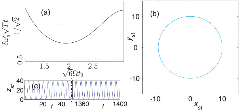
Figure 1: (color online). (a) $\delta\omega^{\prime}_{a}\sqrt{Tt}$ as a function of $\sqrt{6}\Omega t_{3}$, for a partially entangled state obtained by a single application of $H_{I}^{\rm gate}$, Eq. (10) (resonant case) during a time $t_{3}$, that for $t_{3}\simeq 2/(\sqrt{6}\Omega)$ obtains an improvement over the best classical strategy (shot-noise limit, dashed). Shown is also Heisenberg limit, dotted. (b,c) Classical trajectory of the relative coordinates $x_{st}$, $y_{st}$, $z_{st}$. All the spatial coordinates are relative to $\sqrt{\hbar/m\omega_{z}}$, and time to $1/\omega_{z}$.

The Ramsey method has not been used for the one-particle measurements. Instead, a much weaker drive applied over a much longer time was used to drive anomaly transitions at $\omega_{a}^{\prime}$. When performing an experiment using the above protocol on a similar experimental system, the drive strength, and hence the axial excursion of the electrons, must be substantially increased, so it will be necessary to ensure that the resonant frequency does not shift due to the increased oscillation amplitude and drive strength.

The required drive amplitude is determined by the requirement that a single measurement be performed in much less than $t_{\rm dec}$ of Eq. 12. At 300 mK, under the conditions realized thus far with one electron, this decoherence time is 2.3 seconds. We thus assume that we need the duration of each measurement to be 10% of this limit (about 0.23 s). The effective $\pi/2$ pulses must be completed in a much shorter time; we will use $t/10=23$ ms for the following estimates. Completing the second pulse sequence in 23 ms requires a Rabi frequency $\Omega/(2\pi)=57$ Hz. This corresponds to driving the electron to an axial oscillation amplitude of nearly 0.5 mm for the one-electron parameters that have been realized, requiring a 24 V peak-to-peak driving voltage superimposed upon the 100 V trapping potential. Such a large drive and oscillation amplitude is not excluded in principle since very large oscillation amplitudes have been employed for the detection of a single electron. However, this amplitude is about $10^{3}$ times larger than the amplitude used to carry out quantum jump spectroscopy, during which time it is very important to avoid frequency shifts caused by magnetic and electrical gradients in the trap. Careful investigations of the effects of the large oscillatory potential, and the large axial amplitude, will be required to make sure that $\omega_{a}^{\prime}$ is not unacceptably modified.

Similarly, the duration of a measurement must in practice be less than the cyclotron damping time. Cavity-inhibited spontaneous emission has produced damping times as long as 15 seconds GabrielseDehmelt , but damping times less than a second have been used to investigate systematic effects, so care must be taken here. Coherent modifications of the damping time must also be investigated.

We have analyzed all of the neglected terms from the interaction of the drive with the two electron system, including center-of-mass and stretch normal modes. The frequency splitting of center-of-mass and stretch cyclotron mode, of tens of kilohertz, is large enough such that the coupling with the stretch mode will negligibly affect the gate. These terms can indeed be neglected without effect if the couplings $\tilde{\Omega}$ are weak and detunings $\tilde{\Delta}$ are large. Each such term gives a probability of an unintended change in the quantum state proportional to $(\tilde{\Omega}/\tilde{\Delta})^{2}$. All of the terms neglected from $H_{I}$ have $(\tilde{\Omega}/\tilde{\Delta})^{2}<10^{-4}$, and in most cases many orders of magnitude smaller. Thus, the protocol will be negligibly affected by the neglected terms. In addition, numerical simulations that include the full Coulomb interaction (not just the quadratic expansion) confirm that the internal stretch motion undergoes stable oscillations even for very large axial amplitudes [see Fig. 1(b,c)].

VI Requirements for extending to $N$ electrons

For both metrology and quantum information processing, much bigger gains could be achieved by entangling more than two electrons. Up to many millions of electrons can be simultaneously stored in a Penning trap, though coherent control has only been obtained so far with one trapped electron and for the center-of-mass motion of many particles. Extending these methods to many electrons presents several challenges. First, more than two electrons must be cooled to form a Wigner crystal, and the rotation frequency selected to make a planar crystal. Second, new pulse sequences must be devised to make effective $\pi/2$ pulses to entangle the electrons. Although the shot noise limit could likely be surpassed, whether resonant and off-resonant anomaly drives could maximally entangle $N$ electrons remains to be proven. Third, methods to compensate for the finite extent of the electron crystal must be devised, such as the inhomogeneous broadening from spin frequencies that differ due to the $\rho^{2}$ term in the magnetic bottle [Eq. (2)], unless spins on the same circular orbit could be utilized. Fourth, the crystal’s normal mode spectrum must be derived, and modes with frequencies near $\omega_{cm,c}$ must be checked to ensure that their coupling does not produce unacceptable decoherence errors. These questions will be discussed in detail in future work LamataEtAl .

VII Conclusions

In conclusion, we have shown how two electrons could be entangled using a model system whose building blocks have already been demonstrated with one electron. An experimental investigation is now needed to determine the completeness of the model system. An experimental realization of two-electron entanglement would be the significant first entanglement of isolated elementary particles other than photons. A universal two-qubit gate for quantum computing could then be demonstrated, and it may be feasible to improve the measurement precision for the electron magnetic moment by a factor of two. In addition, the realization of two-electron entanglement would be a first step towards learning about and realizing entangled states of larger numbers of electrons for quantum simulators, and much larger precision gains in magnetic moment measurements using quantum metrology protocols.

VIII Acknowledgements

L.L. and G.G. acknowledge funding by Alexander von Humboldt Foundation, and L.L. the support by Spanish MICINN project FIS2008-05705/FIS. We acknowledge support by European IP SCALA and DFG Excellenzcluster NIM, and by the US NSF.

References

- (1) M. Nielsen and I. Chuang, Quantum Computation and Quantum Information (Cambridge University Press, Cambridge, UK, 2000).
- (2) D. Bouwmeester, A. K. Ekert, and A. Zeilinger, eds., The physics of quantum information, Springer, Berlin, 2000.
- (3) D. Hanneke, S. Fogwell, and G. Gabrielse, Phys. Rev. Lett. 100, 120801 (2008).
- (4) An analysis of a quantum processor and quantum simulator based on arrays of microtraps containing one electron each was performed Tombesi .
- (5) L. S. Brown and G. Gabrielse, Rev. Mod. Phys. 58, 233 (1986).
- (6) H. Dehmelt, Rev. Mod. Phys. 62, 525 (1990).
- (7) B. Odom, D. Hanneke, B. D’Urso, and G. Gabrielse, Phys. Rev. Lett. 97, 030801 (2006).
- (8) S. Peil and G. Gabrielse, Phys. Rev. Lett. 83, 1287 (1999).
- (9) B. D’Urso, R. Van Handel, B. Odom, D. Hanneke, and G. Gabrielse, Phys. Rev. Lett. 94, 113002 (2005).
- (10) X.-P. Huang, J. J. Bollinger, T. B. Mitchell, W. M. Itano, and D. H. Dubin, Phys. Plasmas 5, 1656 (1998).
- (11) M. Tavis and F. W. Cummings, Phys. Rev. 170, 379(1968).
- (12) L. Lamata, J.I. Cirac, J. Goldman, and G. Gabrielse, in preparation.
- (13) N. F. Ramsey, Rev. Mod. Phys. 62, 541 (1990).
- (14) J. J. Bollinger, W. M. Itano, D. J. Wineland, and D. J. Heinzen, Phys. Rev. A 54, R4649 (1996).
- (15) V. Giovannetti, S. Lloyd, and L. Maccone, Science 306, 1330 (2004).
- (16) G. Gabrielse and H. Dehmelt, Phys. Rev. Lett. 55, 67 (1985).
- (17) G. Ciaramicoli, I. Marzoli, and P. Tombesi, Phys. Rev. Lett. 91, 017901 (2003); G. Ciaramicoli, F. Galve, I. Marzoli, and P. Tombesi, Phys. Rev. A 72, 042323 (2005); G. Ciaramicoli, I. Marzoli, and P. Tombesi, Phys. Rev. A 75, 032348 (2007); ibid. 78, 012338 (2008); I. Marzoli et al., J. Phys. B 42 (2009) 154010.