Fresh insights on the structure of the solar core

Abstract

We present new results on the structure of the solar core, obtained with new sets of frequencies of solar low-degree p modes obtained from the BiSON network. We find that different methods used in extracting the different sets of frequencies cause shifts in frequencies, but the shifts are not large enough to affect solar structure results. We find that the BiSON frequencies show that the solar sound speed in the core is slightly larger than that inferred from data from MDI low-degree modes, and the uncertainties on the inversion results are smaller. Density results also change by a larger amount, and we find that solar models now tend to show smaller differences in density compared to the Sun. The result is seen at all radii, a result of the fact that conservation of mass implies that density differences in one region have to cancel out density differences in others, since our models are constructed to have the same mass as the Sun. The uncertainties on the density results are much smaller too. We attribute the change in results to having more, and lower frequency, low-degree mode frequencies available. These modes provide greater sensitivity to conditions in the core.

1 Introduction

Helioseismology is now an extremely successful and proven technique, which can be used to infer the structure and dynamics of the interior Sun (see. eg. Antia & Basu 1994; Gough et al. 1995; Basu et al. 2000a, b; Basu 2003; Couvidat et al. 2003; Schou et al. 1998a; Pijpers 2006; Howe 2008, etc.). However, there is still considerable uncertainty about the structure of the solar core.

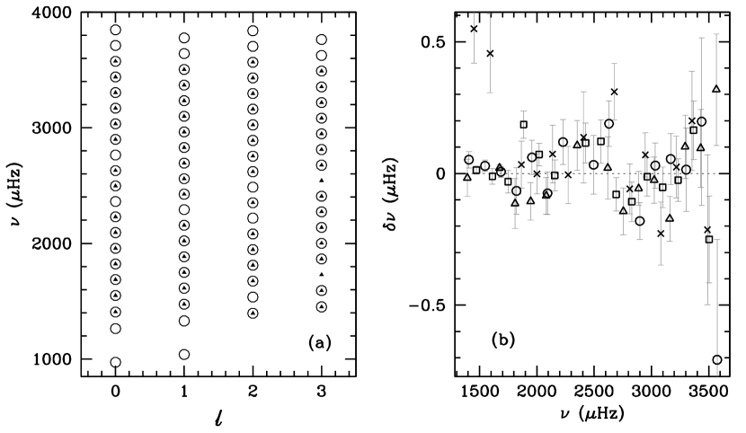
Figure 2: (a) The low-degree $\ell-\nu$ diagram for the BiSON-1 set (circles) and the “Best set” of Basu et al. (1997; triangles). (b) The frequency difference between the BiSON-1 set and the “Best set”. Circles are for $\ell=0$, squares for $\ell=1$, triangles for $\ell=2$ and crosses for $\ell=3$ modes. The differences are in the sense BiSON-1$-$”Best set”.

Different data sets can often give results that show discrepancies. Basu et al. (2000b) found that different solar sound-speed results were obtained depending on whether data from the Michelson Doppler Imager (MDI) or the ground-based Global Oscillation Network Group (GONG) were used. The differences in the inferred sound-speed in the solar core are illustrated in Figure 2 of Bahcall et al. (1998). The sensitivity of the inferred structure to the mode sets has been noted in several investigations (see e.g. Basu et al. 2000a, Turck-Chieze et al. 2001, etc.)

The model fitted to mode peaks in the oscillation power spectrum, as part of the “peak bagging” procedures used to extract estimates of the mode frequencies, can also give rise to discrepant inferences. For example, Toutain et al. (1998) found that sound-speed differences in the core were about 0.2% to 0.3% higher when they used frequencies obtained by fitting asymmetric profiles to the asymmetric peaks in the oscillation power spectrum, rather than what had been the usual practice of fitting symmetric (Lorentzian) profiles. However, Basu et al. (2000a) claimed that the differences were caused by a few unreliable modes, and that the change in frequencies brought about by fitting the more accurate asymmetric profiles would not be expected to affect significantly the inversion results.

So, although the structure of the Sun, in particular the sound-speed profile of the outer 80% by radius, is known very well, the structure of the core is relatively uncertain. The basic reason for this uncertainty is that we only have frequency estimates of acoustic modes, or p modes. The p-modes that probe the inner 0.25${\rm R}_{\odot}$ of the Sun are modes of low-degree $\ell$, i.e., with $\ell=0$, 1, 2 and 3. All solar p-modes have their highest amplitudes close to the solar surface, and hence even modes that probe the core (and there are relatively few of them) are less sensitive to the conditions there than in the outer parts of the solar interior. Frequencies of solar g-modes (buoyancy modes) would help reduce uncertainties, because they have their highest amplitudes in the core. However, g modes are extremely hard to detect, due to their small amplitudes at the solar surface (see e.g., Appourchaux 2008; Appourchaux et al. 2000, 2006; Gabriel et al. 2002; Elsworth et al. 2006). There are recent reports of the possible detection of the signature of several g modes (see e.g., García et al. 2008a, b). There are as yet no convincing candidates for individual g-mode frequencies. Thus, for the moment, we still have to rely on p-modes to determine the structure of the solar core.

The most reliable data on low-degree solar p-modes are obtained from specialized instruments that observe the Sun as a star. The Birmingham Solar-Oscillations Network (BiSON; Chaplin et al. 1996) is a network of such instruments. Data from the network give precise estimates of the frequencies of the low-degree p modes. In this paper we use new sets of data from BiSON to re-examine the structure of the solar core.

To extract information about the solar core properly through inversions of solar frequencies we also need the higher, intermediate-degree modes. Inversions are possible using only low-degree modes, but the results have large errors and the resolution can be poor (see e.g., Basu 2003). While this may be acceptable for other stars, where for the foreseeable future the only modes we can hope to observe are low-degree modes, this is not good enough for the Sun. Unfortunately instruments that determine frequencies of low-degree modes precisely [such as BiSON or GOLF (Gabriel et al. 1997)] cannot determine frequencies of intermediate-degree modes, and instruments that determine frequencies of intermediate-degree modes precisely (such as MDI and GONG) do not obtain as robust frequencies at low degree as BiSON or GOLF. The standard way to overcome this problem is to combine precise low-degree data from one source with precise intermediate-degree data from another. Combining data from different sources requires caution since solar frequencies are known to change with solar cycles (Elsworth et al. 1990; Libbrecht & Woodard 1990; Howe et al. 1999, etc). It has been demonstrated by Basu et al. (1996; 1997) that inverting combined sets when there is a mismatch in the solar activity level of the low- and intermediate-degree data sets can lead to misleading results about the solar core. Thus one either has to use contemporaneous low- and intermediate-degree data; or use a robust method for correcting one of the sets of frequencies to the solar activity level of the other set. Here, we compare results using both approaches.

The intermediate-degree mode frequencies that we use are those estimated by Schou et al. (1998b). This set was obtained from observations made by the MDI instrument on board SoHO during its first year of operation and covers a period from May 9, 1996 to April 25, 1997. The activity level of the Sun was quite low over the entire period that the data were collected, and hence frequency changes over the year in question were not a matter of much concern. The BiSON data sets we use in this paper are contemporaneous with the MDI set. In our 1997 paper (Basu et al. 1997), we had used BiSON data that were nearly contemporaneous with the intermediate-degree data set obtained from the LOWL instrument (Tomczyk et al. 1995). The BiSON data set used then was a combination of frequencies obtained from an 8-month time series, five 2-month time series, and low-frequency data obtained from a 32-month time series. This combined set is referred to in Basu et al. (1997) as the “Best set” and we use the same nomenclature here to refer to this older set. Since 1997 there have of course been improvements in our understanding of the properties of the solar oscillation power spectrum and in the peak-bagging techniques used to extract estimates of the frequencies. As a result, we believe it is time to revisit the question of what the solar core looks like using the BiSON data.

The rest of the paper is organized as follows: We describe our data sets in § 2. The inversion technique and reference models are described in § 3. We present our results in § 4, and discuss their implications in § 5.

2 Data

We use a number of different low-degree sets for this work, most of them obtained with the BiSON instruments. We have, however, also made use of low-$\ell$ frequencies extracted from Sun-as-a-star observations made by GOLF (Bertello et al. 2000, García et al. 2001) and IRIS (Fossat et al. 2003), and from analysis of disc-integrated MDI data (Toutain et al. 1998). The GOLF, IRIS and MDI frequencies are in the literature. The BiSON frequencies come from our analysis of the BiSON data, which is described below. Since the GOLF, IRIS and the disc-integrated MDI data are not contemporaneous with the 360-day MDI intermediate-degree set of Schou et al. (1998b) – which hereafter we shall refer to as data set MDI-1 – for these sets we only use modes with frequencies less than 1800$\mu$Hz. Solar-cycle related changes at these low frequencies are negligible and smaller in size than the uncertainties in the frequencies. The data sets we have used for this work, along with the names we use to identify the sets, are listed in Table 1. All the BiSON sets are supplemented with $\ell\geq 4$ data from MDI-1. The GOLF, MDIlow, and IRIS sets are supplemented with MDI-1 data with $\nu>1800\mu$Hz data for the low-degree modes, and all the higher $\ell$ MDI-1 data.

The majority of the BiSON frequencies came from analysis of data collected over two periods: a 360-day period commensurate with the MDI-1 observations; and a much longer 4752-day period, beginning 1992 December 31 and ending 2006 January 3 (which includes the shorter 360-day period). Estimates of the frequencies of very low-frequency modes came from analysis of datasets prepared specifically to reduce low-frequency background noise (see Appourchaux et al. 2000, and Chaplin et al. 2002, for more details). These ‘low-frequency optimized’ datasets included one dataset prepared from observations made over the 4752-d period; and two others prepared from shorter 2000-day and 3071-day periods within the 4752-day period.

There are two main advantages to using frequencies from the 4752-day period and the other longer periods. First, the frequencies have superior internal precision, e.g., frequency uncertainties in the 4752-day dataset are $\approx 3.5$-times smaller, on average, than those in the 360-day dataset. Second, very low-frequency modes are either more prominent, or only detectable, in the longer datasets.

The main downside to using BiSON frequencies from the longer periods is that they do not cover the same levels of solar activity as the 360-day MDI period. The average activity over the 4752-day period, as determined by various proxies of global activity, is about 60 % higher than the average activity over the 360-day period. Since an increase in surface activity brings with it an increase in mode frequencies, adjustments must be made to the BiSON frequencies to correct them down to values expected for the 360-day period. Only then can the longer-period BiSON frequencies be usefully combined with the 360-day MDI frequencies for inversion.

Solar-cycle variability is much less of a cause for concern in the lower-frequency modes, since, as noted above, they show significantly smaller solar-cycle frequency shifts than their higher-frequency counterparts. We therefore augmented the 360-day BiSON frequency sets with frequencies of very low-frequency modes from the longer BiSON datasets. The GOLF, MDI and IRIS frequency sets that we used were also comprised only of low-frequency modes (having $\nu\leq 1800\,\rm\mu Hz$), and so the impact of the different epochs over which the various data were collected should not have had a significant impact on the modes that we used.

There is one other potential complication for combining the BiSON and MDI frequencies. This complication arises from the fact that BiSON observations are made of the “Sun as a star”. The MDI observations are in contrast made at high spatial resolution. The two types of observation show a marked difference in sensitivity to modes having certain combinations of $\ell$ and the azimuthal order $m$, and as a result the frequencies may show a different response to the azimuthally dependent surface activity.

We now go on to provide more detail on the BiSON analysis, and on the important points raised above. We begin in § 2.1 with a brief summary of how frequencies were estimated from the data. In § 2.2 we discuss how the long-dataset BiSON frequencies were corrected to the activity level of the 360-day MDI period. Then in § 2.3 we explain the inherent mismatch between the BiSON Sun-as-a-star and MDI resolved-Sun data, and the extent to which it is an issue for the frequency data used in our studies, and in § 2.4 we compare the different frequency sets.

2.1 Extraction of mode frequencies from BiSON data

A set of BiSON Sun-as-a-star observations gives a single time series whose power frequency spectrum contains many closely spaced mode peaks. Parameter estimation must contend with the fact that within the non-radial ($\ell>0$) mode multiplets the various $m$ lie in very close frequency proximity to one another. Suitable models, which seek to describe the characteristics of the $m$ present, must therefore be fitted to the components simultaneously. Furthermore, overlap between modes adjacent in frequency means the modes are usually fitted in pairs.

We fitted multi-component models to modes in power frequency spectra of the various BiSON datasets to extract estimates of the mode frequencies. This fitting was accomplished by maximizing a likelihood function commensurate with the $\chi^{2}$, 2-d.o.f. statistics of the power spectral density. We adopted the usual approach to fitting the Sun-as-a-star spectra, and the low-$\ell$ modes were fitted in pairs ($\ell=0$ with 2, and $\ell=1$ with 3). Further background on details of the procedures may be found in Chaplin et al. (1999).

2.2 Correction of long dataset BiSON frequencies to 360-day MDI period

Our procedure for removing the solar-cycle frequency shifts rests on the assumption that variations in certain global solar activity indices may be used as a proxy for the low-$\ell$ frequency shifts, $\delta\nu_{n\ell}(t)$. We assume the correction can be parameterized as a linear function of the chosen activity measure, $A(t)$. When the 10.7-cm radio flux (Tapping & De Tracey 1990) is chosen as the proxy, this assumption is found to be reasonably robust (e.g., Chaplin et al. 2004a) at the level of precision of the data.

Consider then the set of measured BiSON mode frequencies, $\nu_{n\ell}(t)$, that we wish to ‘correct’. Let us take the example where the data come from observations collected over the $t=4752\,\rm d$ period, when the mean level of the 10.7-cm radio flux was $\left<A(t)\right>=121\times 10^{-22}\,\rm W\,m^{-2}\,Hz^{-1}$. Our intention it to correct these frequencies to the mean level of $\left<A(t)\right>_{360}=75\times 10^{-22}\,\rm W\,m^{-2}\,Hz^{-1}$ observed over the 360-day period covered by the MDI data. The mean activity in this 360-day period only just exceeds the canonical quiet-Sun level of the radio flux, which, from historical observations of the index, is usually fixed at $64\times 10^{-22}\,\rm W\,m^{-2}\,Hz^{-1}$ (see Tapping & DeTracey 1990). The magnitude of the solar-cycle correction – which must be subtracted from the raw frequencies – will then be:

$$\delta\nu_{n\ell}(t)=g_{\ell}\cdot{\cal F}[\nu]\cdot[\left<A(t)\right>-\left<A(t)\right>_{360}].$$ (1)

The $g_{\ell}$ are $\ell$-dependent factors that calibrate the size of the shift. These factors are required because the Sun-as-a-star shifts alter significantly with $\ell$ (see § 2.3 below). To determine the $g_{\ell}$, we divided the 4752-day timeseries into 44 independent 108-day segments. The resulting ensemble was then analyzed, in the manner described by Chaplin et al. (2004a), to uncover the dependence of the solar-cycle frequency shifts on the 10.7-cm radio flux. The ${\cal F}[\nu]$ in Equation 1 is a function that allows for the dependence of the shift on mode frequency. Here, we used the determination of ${\cal F}[\nu]$ to be found in Chaplin et al. (2004a, b).

Uncertainty in the correction is dominated by the errors on the $g_{\ell}$. These errors must be propagated, together with the formal uncertainties from the mode fitting procedure, to give uncertainties on the corrected frequencies, $\nu_{n\ell}(t)-\delta\nu_{n\ell}(t)$. The corrected uncertainties are, on average, about 10 % larger than those in the raw, fitted frequencies.

At frequencies below about $\approx 1800\,\rm\mu Hz$, estimated corrections for the 4752-day dataset, and the other long datasets, were smaller in size than the fitted frequency uncertainties. We therefore felt justified in augmenting the 360-day BiSON frequency set with very low-frequency estimates from the longer BiSON datasets.

2.3 On the inherent mismatch between Sun-as-a-star and resolved-Sun frequencies

Extant Sun-as-a-star observations, such as those of the BiSON, are made from a perspective in which the plane of the rotation axis of the Sun is nearly perpendicular to the line-of-sight direction. This means that only components with $\ell+m$ even have non-negligible visibility. Resolved-Sun observations – like MDI – in contrast have good sensitivity to all components in detected modes. Sun-as-a-star and resolved-Sun frequency data must as a result be combined very carefully since there there can be an inherent, underlying mismatch between frequency determinations from the two types of instrument, as will be explained below.

The resolved-Sun data allow for a direct measurement of the frequency centroids of the non-radial modes, because all components are detectable. The frequency centroids carry information on the spherically symmetric component of the internal structure, and are the input data that are required for the hydrostatic structure inversions. In the case of the Sun-as-a-star data, some components are missing, and the centroids must be estimated from the subset of visible components. In the complete absence of the near-surface activity, the $\ell+m$ odd components ‘missing’ in the Sun-a-as-a-star data would be an irrelevance. All mode components would be arranged symmetrically in frequency, meaning centroids could be estimated accurately from the subset of visible components. A near-symmetric arrangement is found at the epochs of the modern cycle minima. However, when the observations span a period having medium to high levels of activity – as a long dataset by necessity does – the arrangement of components is no longer symmetric. The frequencies given by fitting the Sun-as-a-star data then differ from the true centroids by an amount that is sensitive to $\ell$. The $\ell$ dependence arises because in the Sun-as-a-star data modes of different $\ell$ comprise visible components having different combinations of $\ell$ and $|m|$; and these different combinations show different responses (in amplitude and phase) to the spatially non-homogeneous surface activity.

Is it possible to correct the Sun-a-as-a-star frequencies to remove the mismatch? The answer is yes, and the procedure requires knowledge of the strength and spatial distribution of the surface activity over the epoch in question. Chaplin et al. (2004c) and Appourchaux & Chaplin (2007) show how to make the correction, using the so-called even $a$ coefficients from fits for the resolved-Sun frequencies.

Does the mismatch matter for the datasets used here? We should not expect the mismatch to be a cause for concern between the 360-day BiSON frequencies and 360-day MDI frequencies. That is because the surface activity is low throughout this period. We have verified that application of the correction procedure outlined in Appourchaux & Chaplin (2007) does not alter significantly the 360-day BiSON frequencies, nor does it affect significantly the results of the structure inversions.

There will be a more serious mismatch between the 4752-day BiSON frequencies and the 360-day MDI frequencies. However, the solar-cycle frequency correction procedure, outlined in § 2.2 above, adjusts by definition the BiSON frequencies to values expected at low levels of activity; as such this in principle removes the Sun-as-a-star and resolved-Sun mismatch without the need to apply a further correction.

2.4 Comparison of the frequencies

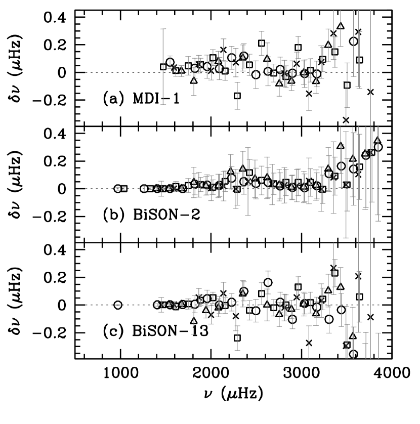
Figure 1: Frequency differences between the BiSON-1 set and: (a) the MDI-1 set; (b) the BiSON-2 set; (c) the BiSON-13 set. The differences are in the sense (BiSON-1$-$ other set. Circles show $\ell=0$, squares show $\ell=1$, triangles show $\ell=2$ and crosses show $\ell=3$ modes.

Panel (a) of Figure 1 shows frequency differences between the BiSON-1 set and the MDI-1 set, while panel (b) of the same figure shows differences between the BiSON-1 set and the BiSON-2 set. The differences in panels (a) and (b) both have the same basic structure. This structure comes from the fact that the BiSON-2 and MDI-1 sets were derived from fits to the oscillation power spectra that used a symmetric (Lorentzian) profile for each mode peak, while the BiSON-1 set came from fits made using a more accurate asymmetric profile. There is also likely to be a contribution to the BiSON-1 minus MDI-1 residuals from differences in the peak-bagging methodologies applied to Sun-as-a-star (BiSON) and resolved-Sun (MDI) data.

The MDI-1 mode set has fewer low-degree modes than the BiSON-1 set, and as a result we would expect to see differences between inversion results obtained by the MDI-1 set and those obtained with BiSON sets supplemented by $\ell\geq 4$ modes from the MDI-1 set. In order to judge the effect of the number of low-degree modes in the set, we have also inverted data using only those modes of the BiSON-1 set that are also present in the MDI-1 set. We call this restricted set the BiSON-1m set for ease of reference.

Differences between the BiSON-1 and 4752-day BiSON-13 set, shown in panel (c) of Figure 1, are on the whole very small because both sets came from asymmetric-profile fits. There are a few $>1\sigma$ outliers, which probably reflect the impact on the fitting of different realization noise in the two sets of data. The observed differences do also increase in size to above $1\sigma$ at high frequencies. This is the part of the oscillation spectrum where the mode peaks are very wide (the modes are heavily damped), meaning the peaks of mode components, and modes, adjacent in frequency begin to overlap. Some modest bias in the estimation of the frequencies can result, and this will be more severe in the shorter BiSON-1 set than in the longer BiSON-13 set because of the inferior frequency resolution of the 360-day BiSON-1 data.

Panel (a) of Figure 2 shows frequency differences between the BiSON-1 and the 1997 “Best set”. As can be seen in the figure, the new BiSON-1 set has filled up some of the gaps in the $\ell-n$ space. Also, the new set extends to somewhat lower as well as higher frequencies. The frequency differences shown in panel (b) of the same figure have a definite structure as a function of frequency, which has a similar pattern to the structure in panels (a) and (b) of Figure 1. These differences are again largely due to the fact that the “Best set” was derived from fits that used a symmetric profile for the mode peaks. It should be noted that some of the difference in the frequencies probably also comes from other improvements to the peak-bagging routines that have been implemented since the mid 1990s.

Since the overall differences are not random, we might again expect to find some differences in the inferred structure of the solar core

3 The inversion technique

Inversion for solar structure is complicated because the problem is inherently non-linear. The inversion generally proceeds through a linearization of the equations of stellar oscillations, using their variational formulation, around a known reference model (see e.g., Dziembowski et al. 1990; Däppen et al. 1991; Antia & Basu 1994; Dziembowski et al. 1994, etc.). The differences between the structure of the Sun and the reference model are then related to the differences in the frequencies of the Sun and the model by kernels. Nonadiabatic effects and other errors in modeling the surface layers give rise to frequency shifts which are not accounted for by the variational principle. In the absence of any reliable formulation, these effects have been taken into account by including an arbitrary function of frequency in the variational formulation (e.g., Dziembowski et al. 1990).

The fractional change in frequency of a mode can be expressed in terms of fractional changes in the structure of model characteristics, for example, the adiabatic sound speed $c$ and density $\rho$, and a surface term. The frequency differences can be written in the form (e.g., Dziembowski et al. 1990):

$${\delta\nu_{i}\over\nu_{i}}=\int_{0}^{R_{\odot}}K_{c^{2},\rho}^{i}(r){\delta c^{2}(r)\over c^{2}(r)}\;{\rm d}r+\int_{0}^{R_{\odot}}K_{\rho,c^{2}}^{i}(r){\delta\rho(r)\over\rho(r)}\;{\rm d}r+{F_{\rm surf}(\nu_{i})\over I_{i}}$$ (2)

Here $\delta\nu_{i}$ is the difference in the frequency $\nu_{i}$ of the $i$th mode between the data and the reference model, where $i$ represents the pair ($n,\ell$), $n$ being the radial order and $\ell$ the degree. The kernels $K_{c^{2},\rho}^{i}$ and $K_{\rho,c^{2}}^{i}$ are known functions that relate the changes in frequency to the changes in the squared sound speed $c^{2}$ and density $\rho$ respectively, and $I_{i}$ is the mode inertia. The kernels for the $(c^{2},\rho)$ combination can be easily converted to kernels for others pairs of variables like $(\rho,\Gamma_{1})$, with no extra assumptions (Gough 1993). The term $F_{\rm surf}$ is the “surface term”, and takes into account the near-surface errors in modeling the structure.

Equation (2) constitutes the inverse problem that must be solved to infer the differences in structure between the Sun and the reference solar model. We carried out the inversions using the Subtractive Optimally Localized Averages (SOLA) technique (Pijpers & Thompson 1992; 1994). The principle of the inversion technique is to form linear combinations of equation 2 with weights $w_{i}(r_{0})$ chosen such as to obtain an average of $\delta c^{2}/c^{2}$ localized near $r=r_{0}$ (the ‘target radius’) while suppressing the contributions from $\delta\rho/\rho$ and the near-surface errors. In addition, the statistical errors in the combination must be constrained. If successful, the result may be expressed as

$$\int{\cal K}(r_{0},r){\delta f_{1}(r)\over f_{1}(r)}{\rm d}r\simeq\sum w_{i}(r_{0}){\delta\omega_{i}\over\omega_{i}}\;,$$ (3)

where the ${\cal K}(r_{0},r)$, the averaging kernel at $r=r_{0}$, is defined as

$${\cal K}(r_{0},r)=\sum w_{i}(r_{0})K_{1,2}^{i}(r)\;,$$ (4)

of unit integral, and determines the extent to which we have achieved a localized measure of $\delta c^{2}/c^{2}$. In particular, the width in $r$ of ${\cal K}(r_{0},r)$, here calculated as the distance between the first and third quartile point, provides a measure of the resolution. Although we attempt to obtain averaging kernels at the target radius $r_{0}$ this is not always possible, and in the core very often the kernel is localized at a different point. This point, unless the averaging kernel is really non-localized, coincides with the second quartile point of the averaging kernel. As a result all our results are plotted as a function of the 2nd quartile points of the averaging kernels obtained at the end of the inversion process. Details of how SOLA inversions are carried out and how various parameters of the inversion are selected were given by Rabello-Soares et al. (1999).

Since the solar core is difficult to invert for, we also inverted the data using the Regularized Least Squares (RLS) technique. Given the complementary nature of the RLS and SOLA inversions (see Sekii 1997 for a discussion), we can be more confident of the results if the two inversions agree. Details on RLS inversions and parameter selections can be found in Antia & Basu (1994) and Basu & Thompson (1996). In this work we invert for the relative difference of the squared sound speed, i.e. $\delta c^{2}/c^{2}$ between the Sun and the reference solar model using $(c^{2},\rho)$ kernel pairs, and for the relative density difference $\delta\rho/\rho$ between the Sun and reference model using $(\rho,\Gamma_{1})$ kernel pairs.

Our main reference model is model BP04 of Bahcall et al. (2005). We also use two other models in the discussion of our results, model S of Christensen-Dalsgaard et al. (1996), and model BSB(GS98) of Bahcall et al. (2006), which in this paper we refer to as simply model BSB. All the models are standard solar models, but have been constructed with somewhat difference input physics. The characteristics and physics inputs of the models are listed in Table 2.

Most of the structure inversion results found in the literature have been obtained with model S as the reference model. However, the input physics in model S is now somewhat outdated, in particular the equation of state is known to have problems under the conditions found in the solar core. The opacities are also somewhat outdated. As a result we use BP04 as our reference model. Model BP04 is very similar to model S, but it is constructed with an improved equation of state and newer opacities. Model BSB is in contrast quite different from the other two models. In particular it uses OP opacities (Badnell et al. 2005) instead of OPAL opacities (Iglesias & Rogers 1996). The OP opacities are somewhat smaller than OPAL opacities for conditions expected in the solar core, but somewhat larger than OPAL opacities at the base of the convection zone. The core structure has also been affected by the new and lower ¹⁴N($p$,$\gamma$)¹⁵O reaction rate (Formicola et al. 2004).

It should be noted that all the models that we use are high-$Z/X$ models, with $Z/X$ values adopted from either Grevesse & Noels (1993) or from Grevesse & Sauval (1998). Asplund et al. (2005) compiled a table of solar abundance determinations based on new techniques that showed that solar metallicity is about 30% lower than previous estimates. This led to large changes in the structure of standard solar models, and in particular, made the agreement between the Sun and solar models much worse [see Basu & Antia (2008) for a review of the problem]. Since the aim of this paper is to take a fresh look into the structure of the Sun rather than study solar models, we restrict ourselves to models that are known to agree well with the Sun.

4 Results

4.1 Sound speed

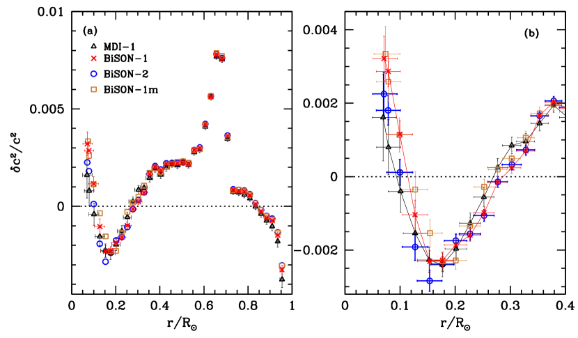
Figure 3: The relative difference in the squared sound-speed between the Sun and reference model BP04 obtained by inverting the different data sets marked in the figure. SOLA inversion results are shown. Panel (a) shows the entire radius range, while panel (b) focuses on the core. The vertical error bars are a measure of the errors in the inversion and come from the uncertainties in the frequencies propagated through the inversion process. The horizontal error bars are a measure of the resolution of the inversions, and are the distance distance between the first and third quartile points of the averaging kernels obtained from the inversions. Only two sets of errors are shown in panel (a) for the sale of clarity. In panel (b) we have joined the points corresponding to MDI-1 and BiSON-1 sets to guide the eye.

The relative differences in the squared sound speed between the Sun and model BP04, as obtained with the different BiSON sets, are plotted in Figure 3. Also plotted is a close-up of the differences in the core. We can see from the figure that the 1-year BiSON sets combined with $\ell\geq 4$ modes from the MDI 360 day set give very similar results, but that the results are different from those obtained with the MDI-1 set, which is the MDI 360-day set for all degrees. The differences between the MDI-1 and BiSON sets are seen below about $0.35R_{\odot}$, where the $\ell=3$ modes begin to influence the results. While we were able to get smaller errors in the inversion results, we were not able to push the inversions much deeper without increasing the errors.

The differences between the MDI and BiSON results are not merely a result of having more modes. If that were so, the result of inverting set BiSON-1m would have been similar to the MDI-1 result. While this is indeed true between about $0.2$ and $0.3R_{\odot}$, in deeper layers the BiSON-1m set gives very similar results to the other BiSON sets, pointing to the fact that the frequencies themselves, as well as the lower errors of the BiSON frequencies, play a rôle.

The sound-speed obtained with the symmetric BiSON-2 set is marginally higher than that obtained with the asymmetric BiSON-1 set, however, the results agree within errors. Since all the 1-year BiSON sets give similar results, and since peaks in the solar oscillation power spectrum are known to be asymmetric, in further discussion of the 360-d BiSON inversions we shall use the results from BiSON-1, not BiSON-2.

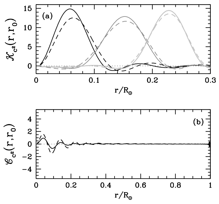
Figure 5: (a) The averaging kernels obtained from the SOLA inversions of the BiSON-13 (solid lines) and BiSON-1 sets (dashed lines). The innermost averaging kernels and two others are shown. (b) The cross-term kernels corresponding to the innermost averaging kernels for the BiSON-13 (solid) and BiSON-1 (dashed) sets.

As far as the BiSON-13 set is concerned, it lets us go marginally deeper into the core, with the innermost averaging kernel centered at 0.062${\rm R}_{\odot}$. We get lower sound speeds than BiSON-1 but higher speeds than MDI-1 in the deepest regions, as is seen in Figure 4. The BiSON-13 results above 0.2 $R_{\odot}$ lie between the BiSON-1 and MDI results; while between 0.1 and 0.2 $R_{\odot}$ they lie slightly above the BiSON-1 and MDI-1 results. Figure 5 shows the innermost averaging kernel, as well as two others obtained with the BiSON-13 and BiSON-1 sets. Also shown are the “cross-term” kernels corresponding to the innermost averaging kernels. Note that the peak of the BiSON-13 averaging kernel is closer to the centre.

Figure 6 shows the sound-speed difference obtained by the BiSON-1 set compared with that of the “Best set” of Basu et al. (1997). We see that the differences in structure are small. With the new set we can though push closer to the core, which we believe is a result of the lower-frequency modes in the new set. One point should be noted: in the Basu et al. (1997) paper, we had plotted the results against the “target” radius, instead of the 2nd quartile point as we have done here. Our experience with inversions in the intervening period leads us to believe that plotting the results against the 2nd quartile point is more correct, since they are the points where the averaging kernels are localized.

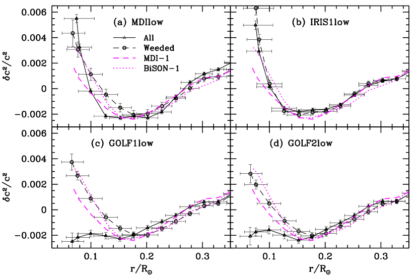
Figure 7: The relative difference in the squared sound-speed between the Sun and reference model BP04 obtained by inverting the low-degree modes obtained with other instruments. The results for MDI-1 and BiSON-1 are shown for comparison. We show two results for each external set: the “All” results are obtained using all the modes, the “Weeded” results are obtained after weeding out modes with large residuals. Since the same set of $\ell>3$ modes are used for all sets, we only focus on the core. Only SOLA inversion results are shown

The BiSON-1 and MDI-1 results are compared with the other data sets listed in Table 1 in Figure 7. For the external data sets, we show two inversions, one marked “All” and the other marked “Weeded.” The inversions marked “All” used all the $\nu<1800\mu$Hz modes in the sets, while the ones marked “Weeded” had a few modes removed, usually because they had large residuals in the RLS inversions. The MDIlow “All” results show a steeper rise in solar sound-speed near the core. However, RLS inversion of this set show that two modes ($\ell=2,n=6$ and $\ell=2,n=7$) had extremely large residuals (16 and 22$\sigma$ respectively). This problem had also been noted earlier by Basu et al. (2000a), who used different reference models. The weeded results are quite similar to the BiSON results. The IRISlow set was problematic in that many modes had high residuals. The worst offenders were the $\ell=1,n=7$, $\ell=1,n=10$ and $\ell=2,n=7$ modes. With these modes in place, the IRISlow data implied that the solar sound-speed increased enormously compared to the reference model at radii below $0.1R_{\odot}$. With these modes removed the results are still higher than the BiSON results, but within 1$\sigma$.

The results for the two GOLF sets are much more interesting. The unweeded results (“All”) show a marked departure from the BiSON and MDI results below 0.15$R_{\odot}$. These two GOLF sets contain very low-frequency detections that are controversial and extremely uncertain, which have not been verified independently by other data. The GOLF1low set set has an $\ell=0,n=5$ mode at $825.202\pm 0.005\mu$Hz and an $\ell=0,n=3$ mode at $535.743\pm 0.003\mu$Hz. The GOLF2low set has an $\ell=0,n=3$ at $535.729\pm 0.009\mu$Hz. The lowest BiSON-1 frequency, for comparison, is the $\ell=0,n=6$ mode at $972.613\pm 0.002\mu$Hz. We note that this mode has been observed in BiSON and GOLF data.

The $\ell=0,n=3$ mode changes the inversion results for the GOLF2low set completely. Given that there are no other modes in the set at comparably low frequencies, this raises a serious question mark over whether this is a real effect. In the absence of this mode, the GOLF2low results (“Weeded” in Figure 7) match the BiSON-1 results almost exactly. The situation is the same with the GOLF1low results. Note that the same inversion parameters have been used for both the “Weeded” and “All” sets. The $\ell=0,n=3$ mode appears to exert a disproportionate influence, the $\ell=0,n=5$ less so, but it also pulls down the solution. Without these two modes, the sound-speed difference obtained is again very similar to that of the BiSON-1 set. We discuss the issue of low-frequency modes further in § 4.2. Thus, if for the moment we ignore the effect of the $\ell=3$, $n=3,5$ modes, it appears that the solar sound-speed still shows a dip in the sound-speed difference with respect to the solar model around $0.2R_{\odot}$ and rises to positive values at radii below $0.1R_{\odot}$. The effect of the two very low-frequency modes in lowering the estimated sound speed in the core has also been noted by Turck-Chieze et al. (2001). The changes between the “All” and “Weeded” results are caused by differences in the inversion coefficients. For SOLA inversions, the modes that were weeded out changed the inversion coefficients of the neighbouring low-degree modes by a large amount. The changes were much smaller in the case of RLS inversions, and because the low-degree modes have large residuals, the changes did not affect the solution.

4.2 Density

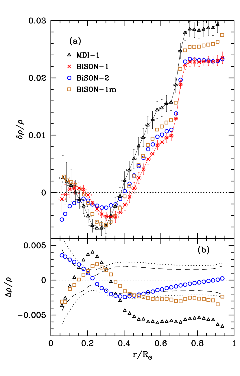
Figure 8: Panel (a): Relative density differences between the Sun and reference model BP04 obtained by inverting the data sets marked in the figure. Only two sets of error bars are shown for the sake of clarity. The errors on the other points are similar to those on the BiSON-1 set. Panel (b): The relative differences in the inferred solar density obtained from the different data sets. The differences are taken with respect to the solar density inferred by using the BiSON-1 set. The dotted line shows the 1$\sigma$ error limit for the MDI-1 set, the dashed line is for the other BiSON sets. Note that there are significant differences in the results. Only SOLA inversion results are shown for the sake of clarity.

The density differences between the Sun and model BP04, as obtained by the different BiSON sets, are shown in Figure 8(a). Also shown in the figure is the result of inverting the MDI-1 set. As can be seen from the figure, the BiSON sets give fairly similar results, within errors. However, the MDI results are different at all radii, not just close to the core. At first glance this is surprising since the only difference between the MDI and BiSON sets are the $\ell<4$ modes, and one would expect differences only in the core, as was found for the sound-speed difference. However, the result is not really surprising. Density inversions are carried out by imposing the condition that the mass of the reference model is the same as that of the Sun. Thus the density differences must integrate out to zero, i.e.,

$$\int 4\pi r^{2}\delta\rho=\int 4\pi r^{2}\rho{\delta\rho\over\rho}=0.$$ (5)

The density $\rho$ in the core is large, and thus a small relative difference $\delta\rho/\rho$ in the core will lead to a large difference in the regions where the density is small. The higher number of low-degree models in the BiSON sets allows us determine the core structure much better than with the MDI set: we find a smaller difference in the core, which implies a smaller difference at all radii. That said, the difference between the BiSON and MDI results is not merely a matter of the larger BiSON mode set. If we only use BiSON frequencies of those modes that are present in the MDI set (i.e., set BiSON-1m), the result lies between the MDI and the other BiSON sets. This can be seen in Figure 8(a). These results show us that when we attempt to infer the solar density it is not enough to have good intermediate and high-degree modes: it is more important to have reliable data on low-degree modes. Given that the BiSON low-degree sets still have gaps and do not yet have very low-frequency modes, we can be sure that solar density results will change if we get better low-degree sets.

In Figure 8(b) we show the relative differences in the inferred solar density obtained from the different sets. The differences are shown with respect to the results obtained with the BiSON-1 set. As can be seen, the differences are completely systematic, even when within errors as is the case for BiSON-2. Judging by the difference between the results of the MDI-1 set and the results of the BiSON sets, we estimate that despite the small statistical errors, solar density inversions are uncertain at a level of about 0.6%. Figure 9 shows the density differences obtained with the BiSON-13 set compared to those obtained with the BiSON-1 and MDI sets. The BiSON-13 set seems to imply a low-density solar core.

Figure 10 compares the density differences obtained using the “Best set” of Basu et al. (1997) and the BiSON-1 set. Note that the density differences obtained with the “Best set” are larger in general, and in the core they imply that the density in the Sun appears to be much greater than in the reference model. This result is in seeming contradiction to the result reported by Basu et al. (1997) (even though that was for a different reference model, the model S), which was that the solar density was found to be much lower than the density in the reference model.

This discrepancy appears to be a result of the use of the $(\rho,Y)$ kernel combination by Basu et al. (1997). Density difference results obtained for the “Best set” using model S as the reference and with $(\rho,\Gamma_{1})$ and $(\rho,Y)$ kernels are shown in Figure 11. With $(\rho,\Gamma_{1})$ kernels we see that the inferred density difference between the Sun and the model is positive in the core. Transformation to kernels involving $Y$ requires the assumption that the equation of state and the heavy element abundance are known exactly. Basu & Christensen-Dalsgaard (1997) showed that the density results obtained with these $(\rho,Y)$ kernels are sensitive to errors in the equation of state assumed for the reference model. Model S was constructed with an equation of state that was found to be deficient for conditions found in the solar core (Elliott & Kosovichev 1998), and as a result we believe that the results obtained using the $(\rho,\Gamma_{1})$ variable combination are more robust than those obtained with $(\rho,Y)$, even though it is at the expense of larger statistical errors. Basu et al. (1997) had discussed the possibility of systematic errors in the density results caused by the particular choice of kernels, but had not tested the results obtained using other sets of kernels.

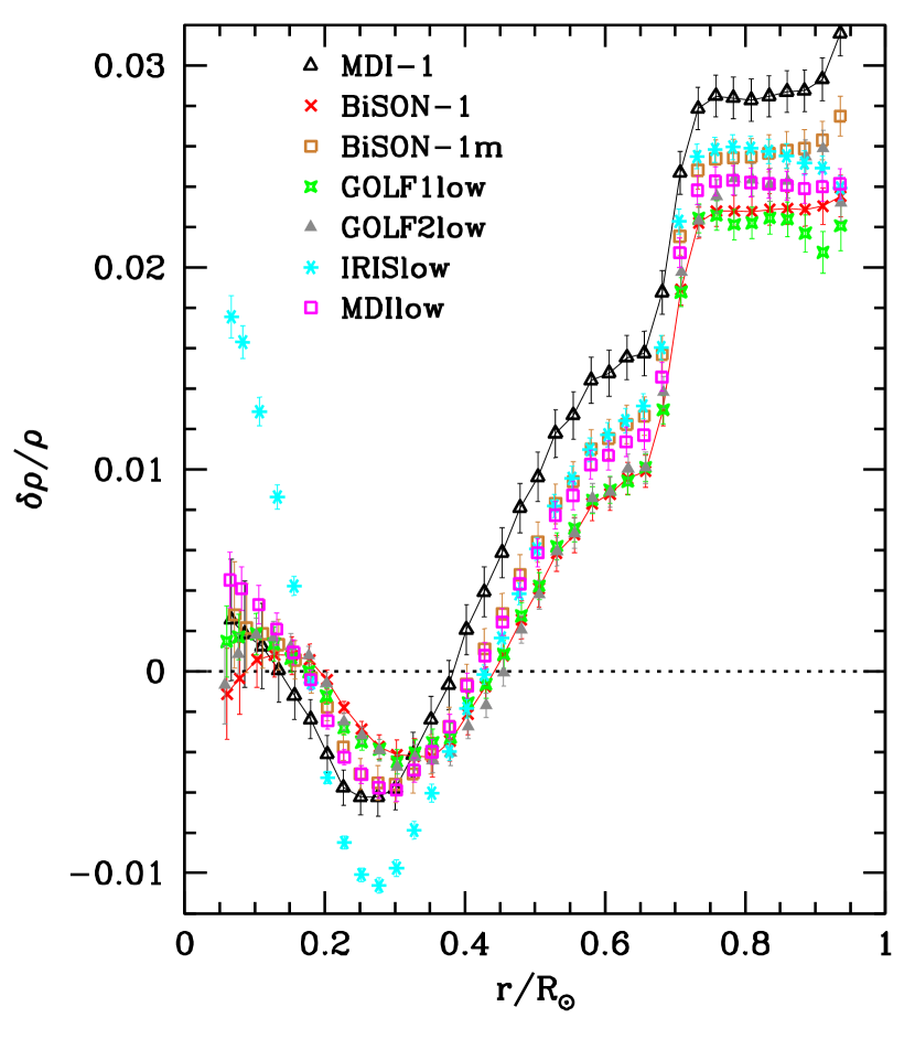
Figure 12: The relative difference in the density between the Sun and reference model BP04 obtained by inverting the low-degree modes obtained with other instruments. The results for MDI-1 and BiSON-1 are shown for comparison. Only the results obtained with the weeded sets are shown. Lines have been drawn through the BiSON-1 and MDI results to guide the eye. Only SOLA inversion results are shown.

Figure 12 shows the density differences obtained for the four external sets — MDILow, IRISLow, GOLF1Low, and GOLF2low. We only show the results of the weeded sets. Although there are differences in the results obtained by the various sets, only set IRISlow gives completely discrepant results, probably implying that some of the frequencies are not accurate. While all other differences lie within a few $\sigma$ there are systematic trends as expected from the conservation of mass constraint (see above). The two GOLF results are again interesting. Although the results obtained from the weeded sets shown in Figure 12 are very similar to those obtained using the BiSON sets, the unweeded results are troublesome. Figure 13 shows both the weeded and unweeded results obtained with the GOLF sets. We show both SOLA and RLS results. The striking feature of the unweeded results is that the SOLA results do not match the RLS results at all. This again leads us to believe that there could be some problems with the very low-frequency $\ell=0$ modes that were weeded out from the two sets. One of the drawbacks of the SOLA method is the implicit assumption that the frequency differences and the errors associated with them are correct. However, sometimes the observational errors can be either under- or over-estimated, or the modes may have unusual characteristics (e.g., much smaller line widths than modes adjacent in frequency), in which case the inversion results can be misleading. RLS inversions are less prone to be affected by such outliers, and hence we are more inclined to believe the RLS results, which agree with the weeded SOLA results.

5 Discussion

We have used a number of BiSON low-$\ell$ data sets, combined with $\ell>3$ data from the MDI 360-day set, to obtain sound speed and density differences between our reference model BP04 and the Sun. We find that we are able to go slightly deeper into the core than we had been able to do with earlier BiSON sets. While the sound-speed results are similar to what we had seen earlier (e.g., Basu et al. 1997), the density results show larger differences. Since the new sets of BiSON frequencies have more modes, and smaller estimated uncertainties, we believe that our current results are more reliable.

Differences in inversion results obtained by using as input frequencies estimated from symmetric and asymmetric fits to the oscillation power spectra are within errors. This is what had also been found for GOLF data by Basu et al. (2000a). Similarly the inversion results obtained from frequencies with and without Sun-as-a-star corrections are very similar. The differences in density results are larger, but although they are systematic, the differences are still within errors. The BiSON-13 set, which has low frequency data from a 4752-day long spectrum, allows us to get results with somewhat smaller errors. The solar sound-speed and density results obtained with this set are tabulated in Table 3.

The sound-speed results are very similar to what has been obtained before, except that we go slightly deeper in the core and the errors are slightly smaller. From Figure 3 we can still see a discrepancy in the sound-speed difference around $0.2{\rm R}_{\odot}$, a large positive difference just below the base of the convection zone, and a gentle fall in the convection zone itself. Of these features, the discrepancy at the base of the convection zone is easiest to interpret. This feature is usually taken as evidence for mixing in the Sun below the base of the convection zone, mixing that is absent in the models (see e.g., Gough et al. 1996; Basu et al. 1996. 1997; etc.). This supposition is supported by inversions for the helium profile of the Sun (Antia & Chitre 1997). Support for this interpretation also comes from the fact that models that incorporate mixing below the base of the convection zone show a reduced discrepancy with respect to the Sun (see e.g., Gough et al. 1996; Basu et al. 2000b). There is also a mismatch in the position of the convection zone base in the Sun ($0.713{\rm R}_{\odot}$; Christensen-Dalsgaard et al. 1991; Basu 1998) and our reference model ($0.7146{\rm R}_{\odot}$), and this also contributes to the discrepancy.

The discrepancy close to the core is more difficult to interpret, but is believed to be related to weak mixing at some time during the Sun’s evolution (see e.g. Gough et al. 1996). The third apparent discrepancy is for $r>0.8R_{\odot}$. Basu et al. (2003) noted that for their reference model, the discrepancy decayed with depth from the surface at a rate roughly proportional to $c^{-1}$. Since they could not find any physical reason for such a discrepancy in what is essentially an adiabatically stratified region, they believed that the feature was a systematic error in the inversions caused by imperfect suppression of the near-surface errors.

Before we try to interpret the features in the sound-speed difference between the Sun and our models, it is instructive to look at differences between different standard solar models and the differences these models show with respect to the Sun. Figure 14 shows the relative sound-speed and density differences between model S and BP04, and between model BSB and BP04. These are exact differences, but convolved with the averaging kernels obtained from inverting set BiSON-1. Convolution with the averaging kernels makes it easier to compare these differences with those obtained from the inversions using the BiSON data. Figures 15 and 16 show the sound speed differences, respectively for all radii and just for the core — between the Sun and models S and BSB; while Figure 17 shows the density differences between these models and the Sun. The first thing to note from Figure 14(a) is that the sound-speed difference between BSB and BP04 has the same type of behavior at $r>0.8R_{\odot}$ as does the sound-speed difference between the Sun and model BP04 (and model S), and in fact the sound-speed differences between the Sun and model BSB are flatter in this region (Figure 15). Yet the model differences are exact and therefore should not suffer from imperfect suppression of near-surface errors. There is a small difference between the convolved and the unconvolved differences that points to effects of the finite resolution of the averaging kernels, but the effect of finite resolution is to reduce the sound-speed difference for $r>0.8R_{\odot}$. The difference between the sound-speed profiles of BSB and BP04 in the convection zone is a result of using different low-temperature opacities (Ferguson et al. 2005 in BSB and Alexander & Ferguson 2004 in BP04). Although, the bulk of the convection zone is stratified adiabatically, the structure closer to the surface is affected by differences in low-temperature opacities, which is manifested as the observed sound-speed differences in the convection zone of these models. This occurs predominantly because of differences in the mixing length parameter needed to model the present-day Sun. In particular, we find that the mixing length parameter is 2.19 when OPAL opacities are used in conjunction with the low-temperature opacities of Ferguson et al. (2005); is 2.21 when OPAL opacities are replaced by OP opacities; and is 2.11 when we use a combination of OP opacities and the Alexander & Ferguson (1994) low-temperature opacities. Therefore, we conclude that the differences in sound-speed between the Sun and our models in the convection are most likely to be due to deficiencies of our models and not merely due to limitations of our inversion techniques.

The next prominent feature in Figure 14(a) is the increased difference just below the base of the convection zone. While at first glance this is reminiscent of the increase in Figures 3 and 15, a careful look shows that the difference actually occurs over a wider radius range, and is also smaller than the difference between the Sun and BP04. The differences between the models can basically be attributed to differences in opacity. In the case of model S and BP04, both the convection-zone heavy element abundance and the opacity tables used are different. BP04 effectively has lower opacity (and hence a shallower convection zone) than model S. While BP04 and BSB have the same convection-zone metallicity, BSB used OP rather than OPAL opacities. OP opacities are marginally larger than OPAL opacities for conditions present at the base of the convection zone and that caused the small spike in the sound-speed difference between these two models. These differences do not explain the larger, and more localized, sound-speed difference between the Sun and the three models. Mixing below the solar convection zone remains the best explanation, and as mentioned earlier, there is other evidence for mixing in this region (e.g., Antia & Chitre 1997).

Going back to the sound-speed differences between the Sun and models BP04, S and BSB at the core, we can see the solar sound-speed differences against all three models show a localized dip around $0.2{\rm R}_{\odot}$, implying that the solar sound-speed is lower than that of the models. At even smaller radii the sound-speed in the Sun appears to be larger than the sound-speed in the models, at least for the case of models S and BP04. This feature, particularly in the case of model S, has been used as evidence for possible mixing at some time in the Sun’s past (see Gough et al. 1996). While mixing in the past is a possibility, the evidence is somewhat less compelling when models with more updated physics are used. For example, if we look at the sound-speed differences between the Sun and model BSB, the large, positive difference in the core is reduced in size. However, the deficit around $0.2{\rm R}_{\odot}$ remains, although it is shifted inwards and is closer to $0.15{\rm R}_{\odot}$. Basu et al. (2000a) had claimed that the dip in the sound-speed difference is independent of the reference model and hence intrinsic to the Sun, but it appears that their result was due to the fact their various reference models used very similar physics inputs. The difference in the reaction rates and opacities in BSB compared to those in models S and BP04 are evidently large enough to shift the position of the deficit. Thus, we might expect models with newer inputs to show other changes. Also notable is that the sound speed difference between BSB and BP04 (see Figure 14) shows a larger sound-speed in model BSB at low radii, and a lower sound speed around $0.3{\rm R}_{\odot}$. These differences are purely due to changes in input microphysics, i.e., opacities as well as nuclear reaction rates.

Of course, the conjecture that there may have been mixing in the solar core was not based on sound-speed inversions alone. Gough et al. (1996) used the density inversion results as corroboration. One should note, however, that the density difference that Gough et al. (1996) used was obtained with $(\rho,Y)$ kernels, and like the $(\rho,Y)$ result shown in Figure 11, showed that density of the solar core is less than the density in model S in the core. Gough et al. (1996) argued that the relatively steep positive gradient in $\delta\rho/\rho$ in the core and immediately beneath the convection zone imply that the magnitude of the negative gradient of density is too high in the model. However, our more robust inversions show that the gradient of $\delta\rho/\rho$ is not steep for any of the three models, and not positive for models BP04 and BSB.

Thus, we find that even with improved data, interpreting the sound-speed and density differences against different models is not completely straightforward. Improvements in solar models need to go hand-in-hand with improvements in the observational data. To be able to invert closer to the solar core we require reliable frequency estimates of very low-$n$, low-degree modes. Since these modes have large amplitudes close to the core, they will help (even in the absence of g-modes) to get a better handle on the innermost layers if the Sun. As we have seen in this paper, changes in the low-degree mode set can lead to large variations in estimated density differences between reference solar models and the Sun. There is therefore a clear need for very low-frequency modes if we are to obtain robust, precise density estimates for the Sun.

Table 1: Frequency datasets used for the inversions

Dataset	Comments	Reference
MDI-1	$0\leq l\leq 150$	Schou et al. (1998)
BiSON-1	1 yr, asymmetric fitting
BiSON-1m	Same as BiSON-1, but restricted to the
	same low-$\ell$ modes as MDI-1
BiSON-2	1 yr, symmetric fitting
BiSON-13	13 yr, asymmetric fitting, solar-cycle corrected
GOLF1low	$\nu\leq 1800\,\rm\mu Hz$	Bertello et al. (2000)
GOLF2low	$\nu\leq 1800\,\rm\mu Hz$	Garcia et al. (2001), Table V
MDIlow	$\nu\leq 1800\,\rm\mu Hz$	Toutain et al. (1998)
IRISlow	$\nu\leq 1800\,\rm\mu Hz$	Fossat et al. (2003)

Table 2: Inputs and characteristics of reference solar models

		Model
	BP04	S	BSB
Inputs:
Mass	$1.989\times 10^{33}$g	$1.989\times 10^{33}$g	$1.989\times 10^{33}$g
Radius	$6.9598\times 10^{10}$cm	$6.96\times 10^{10}$cm	$6.9598\times 10^{10}$cm
Luminosity	$3.8418\times 10^{33}$ erg/s	$3.846\times 10^{33}$ erg/s	$3.8418\times 10^{33}$ erg/s
(Z/X)sur	0.0229	0.0245	0.0229
	Grevesse & Sauval (1998)	Grevesse & Noels (1993)	Grevesse & Sauval (1998)
Eq. of State	OPAL	OPAL	OPAL
	Rogers & Nayfonov (2002)	Rogers et al. (1996)	Rogers & Nayfonov (2002)
Opacity	OPAL	OPAL	OP
	Iglesias & Rogers (1996)	Rogers & Iglesias (1992)	Badnell et al. (2005)
	Alexander & Ferguson (1994)	Kurucz (1991)	Ferguson et al. (2005)
Reaction rates	Bahcall &	Bahcall &	Bahcall &
	Pinsonneault (2004)	Pinsonneault (1995)	Pinsonneault (2004)
			Formicola et al. (2004)
Diffusion rates	Thoul et al. (1994)	Proffitt &	Thoul et al. (1994)
		Michaud(1991)
Characteristics:
$Y_{\rm CZ}$	0.243	0.247	0.243
$R_{\rm CZ}$	0.7146	0.7129	0.7138

Table 3: Solar sound-speed and density profiles as derived from BiSON-13

$r/R_{\odot}$	$c$ (cm $s^{-1}$)	$\sigma_{c}$ (cm $s^{-1}$)	$r/R_{\odot}$	$\rho$ (g cm-3)	$\sigma_{\rho}$ (g cm-3)
6.1949E-02	5.1170E+07	9.2178E+03	5.8884E-02	1.2078E+02	1.1601E-01
7.4948E-02	5.1169E+07	4.3834E+03	7.7225E-02	1.0532E+02	7.7585E-02
1.0052E-01	5.0803E+07	4.9108E+03	1.0208E-01	8.5937E+01	5.1525E-02
1.2733E-01	4.9858E+07	4.4274E+03	1.2706E-01	6.9226E+01	3.1670E-02
1.5208E-01	4.8559E+07	4.4193E+03	1.5162E-01	5.5510E+01	2.0105E-02
1.7636E-01	4.7033E+07	3.5829E+03	1.7709E-01	4.3772E+01	1.2053E-02
2.0184E-01	4.5316E+07	3.4470E+03	2.0233E-01	3.4221E+01	6.9189E-03
2.2746E-01	4.3569E+07	3.0592E+03	2.2730E-01	2.6514E+01	4.6064E-03
2.5253E-01	4.1897E+07	2.8858E+03	2.5277E-01	2.0234E+01	4.3910E-03
2.7771E-01	4.0301E+07	2.5884E+03	2.7803E-01	1.5355E+01	4.5718E-03
3.0320E-01	3.8798E+07	2.4506E+03	3.0333E-01	1.1570E+01	3.9911E-03
3.2847E-01	3.7395E+07	2.3018E+03	3.2879E-01	8.6838E+00	3.2633E-03
3.5370E-01	3.6090E+07	2.1119E+03	3.5403E-01	6.5346E+00	2.5846E-03
3.7912E-01	3.4866E+07	1.9529E+03	3.7946E-01	4.9123E+00	1.9819E-03
4.0439E-01	3.3710E+07	1.8638E+03	4.0474E-01	3.7160E+00	1.5338E-03
4.2970E-01	3.2629E+07	1.7383E+03	4.3006E-01	2.8201E+00	1.1410E-03
4.5504E-01	3.1604E+07	1.6411E+03	4.5535E-01	2.1521E+00	8.9351E-04
4.8031E-01	3.0634E+07	1.5152E+03	4.8063E-01	1.6517E+00	6.7778E-04
5.0566E-01	2.9712E+07	1.4385E+03	5.0592E-01	1.2737E+00	5.4124E-04
5.3096E-01	2.8822E+07	1.3808E+03	5.3121E-01	9.8850E-01	4.1931E-04
5.5630E-01	2.7972E+07	1.3146E+03	5.5651E-01	7.7054E-01	3.3861E-04
5.8160E-01	2.7130E+07	1.2604E+03	5.8181E-01	6.0445E-01	2.6438E-04
6.0693E-01	2.6311E+07	1.1919E+03	6.0711E-01	4.7634E-01	2.1495E-04
6.3223E-01	2.5483E+07	1.1390E+03	6.3243E-01	3.7756E-01	1.6995E-04
6.5754E-01	2.4637E+07	1.0619E+03	6.5772E-01	3.0095E-01	1.4047E-04
6.8283E-01	2.3706E+07	1.0045E+03	6.8304E-01	2.4197E-01	1.1334E-04
7.0811E-01	2.2614E+07	9.3680E+02	7.0838E-01	1.9685E-01	9.3937E-05
7.3337E-01	2.1257E+07	8.9853E+02	7.3371E-01	1.6281E-01	7.8683E-05
7.5869E-01	1.9881E+07	8.7096E+02	7.5903E-01	1.3311E-01	6.5124E-05
7.8404E-01	1.8495E+07	7.7763E+02	7.8435E-01	1.0703E-01	5.4001E-05
8.0934E-01	1.7089E+07	7.3027E+02	8.0967E-01	8.4315E-02	4.3385E-05
8.3464E-01	1.5649E+07	6.8648E+02	8.3499E-01	6.4667E-02	3.4486E-05
8.5995E-01	1.4156E+07	6.1451E+02	8.6031E-01	4.7800E-02	2.6671E-05
8.8527E-01	1.2582E+07	5.7896E+02	8.8564E-01	3.3507E-02	1.9704E-05
9.1060E-01	1.0881E+07	5.9297E+02	9.1096E-01	2.1657E-02	1.4339E-05
9.3590E-01	8.9771E+06	5.5548E+02	9.3628E-01	1.2157E-02	9.5495E-06
9.5661E-01	7.1388E+06	4.9286E+02	9.5754E-01	5.9835E-03	6.2548E-06

Figure 4: The relative difference in the squared sound-speed between the Sun and reference model BP04 obtained by inverting set BiSON-13. SOLA inversion results are shown. For comparison, we also show results from sets MDI-1 and BiSON-1.

Figure 6: The relative difference in the squared sound-speed between the Sun and reference model BP04 obtained by inverting the “Best set”. SOLA inversion results are shown. For comparison, we also show results from set BiSON-1.

Figure 9: Panel (a): Relative density differences between the Sun and reference model BP04 obtained by inverting set BiSON-13. Results for MDI-1 and BiSON-1 are shown for comparison. Panel (b): The relative differences in the inferred solar sound speed obtained using the BiSON-1 set and the BiSON-13 set. Results for MDI-1 are shown for comparison. The dotted line shows the 1$\sigma$ error limit for the MDI-1 set, the dashed line is for the BiSON-13 set. Only SOLA inversion results are shown.

Figure 10: The relative difference in the density between the Sun and reference model BP04 obtained by inverting the “Best set”. The results obtained from BiSON-1 are shown for comparison. Only SOLA inversion results are shown.

Figure 11: The relative difference in the density between the Sun and reference model S obtained by obtaining by inverting the “Best set”. Two results are shown, one obtained using the $(\rho,Y)$ kernel combination, the other using the $(\rho,\Gamma_{1})$ kernel combination. Note the striking differences between the two results, especially in the core. Only SOLA inversion results are shown.

Figure 13: The relative difference in the density between the Sun and reference model BP04 obtained by inverting the two GOLF sets. Both RLS (lines) and SOLA (points) inversion results are shown. Note that for the weeded sets the RLS and SOLA results match, while there is a large difference between RLS and SOLA results when all the modes are used. It should be noted that the same inversion parameters were used for both the “Weeded” and “All’ sets.

Figure 14: The relative differences in squared sound speed (panel a) and density (Panel b), between model S and BP04 and model BSB and BP04. The results are in the sense S$-$BP04 and BSB$-$BP04. The lines are the exact differences. The points are the exact differences convolved with the averaging kernels obtained by inverting BiSON-1. Thus, the points are what we would expect to see if we inverted the frequency differences between the models. The differences between the points and the lines are caused by the finite width of the averaging kernels as well as by any non-local features that they may have.

Figure 15: The relative differences in squared sound speed between the Sun and model S (panel a) and model BSB (panel b) obtained by inverting the MDI-1, Bison-1 and BiSON-13 sets. Only SOLA inversion results are shown.

Figure 16: The same as Figure 15, but focusing on the solar core. Only SOLA inversion results are shown.

Figure 17: The relative density differences between the Sun and model S (panel a) and the Sun and model BSB (panel b), obtained from different data sets. Only SOLA inversion results are shown.