Measurement of optical turbulence in free atmosphere above Mt.Maidanak in 2005-2007

Abstract

Results of 2005-2007 campaign of measurement of the optical turbulence vertical distribution above Mt. Maidanak are presented. Measurements are performed with the MASS (Multi-Aperture Scintillation Sensor) device which is widely used in similar studies during last years at several observatories across the world. The data analysis shows that median seeing in free atmosphere (at altitudes above 0.5km) is $0\hbox{$.\!\!^{\prime\prime}$}46$ and median isoplanatic angle is $2\hbox{$.\!\!^{\prime\prime}$}47$. Given a rather long atmospheric coherence time (about 7 ms when the seeing is good) such conditions are favorable for adaptive optics and interferometry in the visible and near-IR.

Accepted for publication in Astronomy Letters, Volume 35, 2009

Key words: astroclimate, seeing, adaptive optics

 
^∗ e-mail: $<$victor@sai.msu.ru$>$

1 INTRODUCTION

Studies of atmospheric optical turbulence have progressed significantly in the last decade. This was stimulated by new programs of site testing for extra-large telescopes. It was also realized that the potential of existing observatories may be further enhanced by the use of adaptive optics (AO) systems.

It is well known that knowledge of only the integral turbulence on the line of sight is not enough for correct prediction of AO efficiency at a given site. Information on the vertical distribution of turbulence is needed for the development of a particular kind of AO (see for example, Vernin et al., 1991; Roddier, 1999; Wilson et al., 2003; Fuensalida et al., 2004; Tokovinin et al., 2003a). It is also well known that atmospheric limits on photometric and astrometric precision are directly linked to the vertical profile of turbulence (Dravins et al., 1997; Kenyon et al., 2006; Shao & Colavita, 1992). It is worth noting that the discussion of this issue in the 1970–80th was mainly related to the selection of optimal height of telescope towers.

Astroclimate parameters of Maidanak observatory were studied for many years. One such campaign was conducted in 1998–99, as reported by Ilyasov et al. (1999) and Ehgamberdiev et al (2000). First estimates of the contribution of free atmosphere to seeing were made by (Kornilov & Tokovinin, 2001) based on stellar scintillation analysis. It turned out that this contribution was quite significant, about 30%.

The development of an effective technique to study vertical turbulence distribution by stellar scintillations (Tokovinin & Kornilov, 2002; Kornilov et al., 2003; Tokovinin et al., 2003b) and of respective instrumentation allowed us to initiate in 2005 the project of turbulence monitoring at Mt. Maidanak during 2–3 years, completed in 2007. Here we report its main results.

2 MEASUREMENT METHOD AND MULTI-APERTURE SCINTILLATION SENSOR (MASS)

The measurement of the altitude distribution optical turbulence is based on the fact that amplitude of stellar scintillation produced by a turbulent layer depends on its height in a different way when observed through different apertures.

As well described in Tatarskiy (1967); Roddier (1981), stellar scintillation is produced by phase fluctuations of a light wave passing through optically turbulent layers of atmosphere, and subsequent propagation. The strength and spatial spectrum of amplitude fluctuations produced by the atmosphere depend on the propagation length.

Scintillation is quantified by the scintillation index $s^{2}$ representing the relative variance of flux in some aperture. Tokovinin (1998) generalizes this concept to the case of simultaneous measurement of fluxes in two different apertures. The two kinds of scintillation indices – so called “normal” and differential – can be directly measured. On the other hand, these indices equal integrals of the turbulence distribution along the line of sight with some weighting functions. The weights are computed from the known aperture sizes and spectral energy distribution of the light. It should be noted that the validity of the small-perturbations method and of the Kolmogorov turbulence spectrum is essential here. In typical conditions of astronomical observations, both these assumptions are usually valid.

Further development of this method is described in papers by Kornilov et al. (2003) and Tokovinin et al. (2003b), where specific algorithms of restoration of turbulence along the line of sight are presented and various instrumental factors are accounted for. As dedicated studies show (Tokovinin & Kornilov, 2007; Kornilov et al., 2007), the precision of turbulence strength representation by a set of six altitude layers is definitely better than 10%. An independent cross-check of these results at some observatories (Fuensalida et al., 2007; Sadibekova et al., 2006) was made with a SCIDAR device (Scintillation detection and ranging, Azouit & Vernin, 1980; Fuchs et al., 1998).

Table 1: MASS entrance aperture diameters ( $d_{I}$ — inner diameter, $d_{O}$ — outer diameter).

Channel	Segmentator mirrors		Effective aperture
MASS	$d_{I}$, mm	$d_{O}$, mm	$d_{I}$, cm	$d_{O}$, cm
A	—	1.03	—	1.60
B	1.05	1.90	1.62	2.93
C	1.95	3.60	3.00	5.54
D	3.65	6.75	5.62	10.4

The MASS device is simply a fast 4-channel photometer which measures fluctuations of the light flux from some reasonably bright star in four concentric apertures from 2 to 10 cm diameters. Detailed description of the device is given by Kornilov et al (2003). Any 5- to 6-inch telescope of about 3m focal distance and without central obscuration may be used as a feeding optics.

A natural drawback of the MASS method is its insensitivity to turbulence near the ground. In order to include it for accessing complete turbulence integral along the line of sight (giving the seeing measure), one has to use some other method, for example differential image motion monitor (DIMM, Sarazin & Roddier, 1990). It is worth recalling here that image quality (seeing) is defined as a full-width at half-maximum of a long-exposure stellar image created by a large aberration-free telescope. Seeing produced by the whole atmosphere without a contribution from the ground layer is referred to as free atmosphere seeing $\beta_{free}$. A reliable estimate of this quantity is normally obtained for turbulence above $h=0.5\mbox{km}$ (Kornilov et al., 2003; Tokovinin et al., 2003b).

The altitude distribution of turbulence above Mt. Maidanak was studied with help of so-called original MASS device of first generation which was designed and built in 2001–2002 in the Sternberg Astronomical Institute in collaboration with the Cerro Tololo and European Southern observatories.

3 MAKING MEASUREMENTS AND SUPPLEMENTARY STUDIES

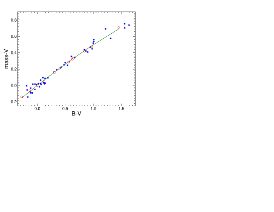
Figure 1: Colour equation of MASS at the refractor telescope AFR-2. Asterisks – real stars, a solid curve – parabolic approximation, circles – computed colour dependencies for a set of used typical spectral energy distributions after the applied response curve correction.

The observations with the MASS were made from August 2005 to November 2007. The device was attached to the photographic refractor telescope AFR-2 of 23 cm aperture and f/no 10. Valid data are only obtained after a proper adjustment of the Fabry lens which sets the sizes of effective work apertures projected onto the telescope entrance aperture plane (Kornilov et al., 2003, 2007). The respective magnification factor equal to 15.4 was measured after installation and was confirmed by repetitive measurements in 2006. The physical sizes of the MASS segmentator and the effective apertures of respective channels are given in Table 1. One can see that aperture size for the channel A is smaller than a typical Fresnel radius $\sqrt{\lambda H}$ = 3 – 7 cm depending on turbulence height while the D-channel aperture is larger which is a must for successful application of profiles restoration algorithms.

The weighting functions converting the turbulence distribution along the line of sight into scintillation indices depend on spectrum of light. Correct account of this factor is implemented using typical energy distributions in spectra of program stars and carefully the measured response curve of the device. While the device itself is well studied in a laboratory, the refractor lens introduces significant absorption in the blue and hence strongly violates the actual response. Correction of this effect was made using photometric measurements of some 50 stars taken 15 and 16 October 2006.

Using the obtained atmospheric extinction coefficient ($0^{m}\!.27$ in the MASS bandpass), the colour equation $mass-V$ vs $B-V$ was constructed (Fig. 1). The slope of this relation allowed us to correct the response of the system given an assumed typical glass selective absorption law. The original MASS response curve and those after correction are shown in Fig. 2.

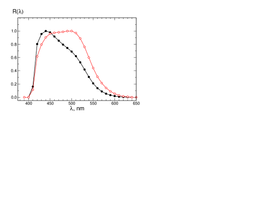
Figure 2: Original (black dots) and corrected (empty circles) spectral response curves of a MASS $+$ telescope system.

Unbiased estimation of turbulence strengths, especially when it is weak, is only possible given the correctly measured detector non-poissonity factors $p$ in A and B channels. The flux in C and D apertures is normally strong enough to neglect this effect. Non-poissonity measurements involve the control light source which is built into the device (Kornilov et al., 2007; Tokovinin & Kornilov, 2007). Control measurements give also the non-linearity (dead-time) measure $\tau$ which, contrary to $p$, is most important for C and D channels where bright stars may develop more than $10^{6}$ counts per second. The results of these supplementary measurements made in two separate nights of 2006 are given in Table 2.

Table 2: The device parameters $p$ (non-poissonity) and $\tau$ (non-linearity) by channels measured in 2006.

Channel	$p$	$\sigma_{p}$	$\tau$, ns	$\sigma_{\tau}$, ns
A	1.010	0.001	22.8	3.5
B	1.012	0.001	21.4	1.4
C	1.008	0.001	21.0	0.3
D	1.007	0.001	19.4	0.2

The statistics of observation time distribution by seasons is given in Table 3. A total of 280 nights was occupied by measurements of which a small fraction (25 nights) were instances of short estimates of less than half an hour duration. Total measurement time is 1022 hours. The gap in June – September 2006 is due to device temporal failure.

Table 3: Measurement duration in nights and hours by months of 2005 – 2007

Season	2005		2006		2007
Months	nights	hours	night	hours	night	hours
January	—	—	—	—	1	0.1
February	—	—	8	20.5	4	15.5
March	—	—	12	27.2	6	8.8
April	—	—	17	71.6	6	15.7
May	—	—	23	84.1	10	23.5
June	—	—	—	—	2	4.8
July	—	—	—	—	26	72.5
August	14	58.8	—	—	25	87.8
September	30	210.0	—	—	21	105.1
October	23	73.8	14	15.9	20	61.4
November	5	34.2	5	9.6	7	18.5
December	—	—	—	—	—	—

Inspite of significant gaps in measurement periods, the observation time distribution follows more or less a typical seasonal clear nights allocation at Mt. Maidanak except for December and January when, by various reasons, no scintillation was measured. The pronounced grouping of measurements in the five periods is well seen: fall 2005, spring and autumn 2006 and the ones of 2007.

An example of MASS measurement results is shown in Fig. 3 for a typical night of September 9, 2005. The sporadic, usually quite short-term, increase of turbulence strength is seen in different layers (altitudes). The turbulence evolved from the evening time gradually declining in altitude. The end of night is dominated by the turbulence at 4 km.

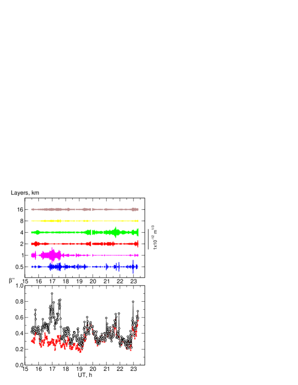
Figure 3: The September 9, 2005 results. Top: six fixed altitude layer representation of turbulence (see section 4). The stripe width is proportional to the layer power which scale is shown by the vertical bar to the right of the graph. Bottom: free atmosphere seeing $\beta_{free}$ behavior (circles) during the night; crosses depict seeing $\beta_{2}$ formed above 2 km.

During the campaign the Maidanak observatory differential image motion monitor (DIMM) was mainly used in other sites of Uzbekistan. Simultaneous measurements with both devices were made in 2005 from 17 of September to 5 of November (18 nights), in 2006 – from 11 of February to 31 of May (24 nights) and continuously during 24 nights from 25 of August to 16 of September of 2007. The results of MASS and DIMM data inter-comparison will be presented in a separate paper.

4 BASIC MEASUREMENT RESULTS

The MASS device is working under the Turbina program control (Kornilov et al., 2003) which operates under Linux OS. Although the functionality of this program includes not only the measurement control but also the real-time data processing spanning from scintillation indices calculation to the restoration of a current altitude turbulence profile, the repetitive off-line data reprocessing allows one to obtain more reliable and homogeneous results. This improvement is related to temporal drifts of the device parameters over 2 – 3 year period and, more importantly, to the continuous software update throughout the campaign time.

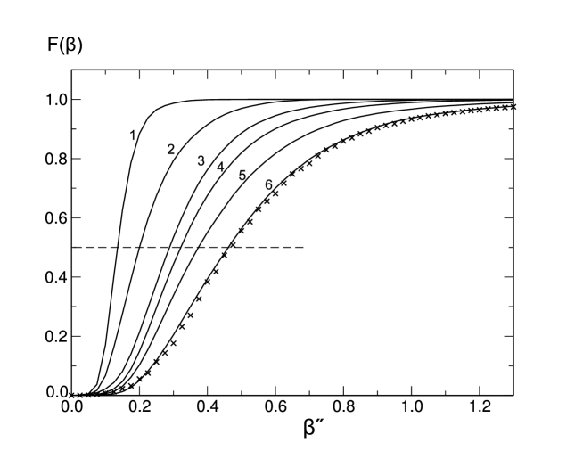
Figure 4: Cumulative distribution of the atmosphere layers input into the image quality: 1 — 16 km layer, 2 — 8 km layer and above, 3 — 4 km and above, 4 — 2 km and above, 5 — 1 km and above, 6 — all atmosphere from 0.5 km and above ($\beta_{free}$). Crosses — $\beta_{free}$ distribution obtained directly from scintillation indices without profile restoration.

Such a reprocessing was performed with help of a special version of an Atmos program which is part of Turbina software, and a set of shell-scripts which filter out the input data glitches and invalid output. Although observations were performed with data accumulation time for a single profile restoration equal to 20 s due to imperfect tracking of AFR-2, the data reprocessing has regrouped the input into commonly accepted 1 min accumulation time.

As an outcome, more than 50 thousand integral atmosphere parameters sets and altitude profiles were computed. Each profile is quantified by turbulence intensities of six layers which are centered at 0.5, 1, 2, 4, 8 and 16 km. It should be stressed that provided values are not $C_{n}^{2}(h_{i})$ but the integrated ones: $J_{i}=C_{n}^{2}(h_{i})\Delta h_{i}$. Hence the input of each layer into the image quality $\beta$ is defined by the following relation: $\beta_{i}=2.0\times 10^{7}\cdot J_{i}^{3/5}$ for wavelength $\lambda=500$ nm. The seeing of $1\hbox{$.\!\!^{\prime\prime}$}0$ corresponds to the integral turbulence strength $J=6.8\times 10^{-13}\mbox{m}^{1/3}$, and $\beta=0\hbox{$.\!\!^{\prime\prime}$}5$ is produced by $J=2.14\times 10^{-13}\mbox{m}^{1/3}$.

In Fig. 4 we show the cumulative distributions of the inputs of different atmosphere parts into the image quality. In other words, it shows the seeing for an observer at a given altitude above the site. Additionally the free atmosphere seeing $\beta_{free}$ distribution is shown, which was calculated as integral atmosphere parameter without profile restoration. One can see that these distributions are statistically indistinguishable.

The median layers contributions are given in Table 4. As a good comparison, the last column shows the median turbulence distribution for a Cerro Tololo observatory quoted from a paper by Tokovinin et al (2003a).

Table 4: Median contribution of atmosphere layers into the image quality (arcseconds).

Layer	Median $\beta$	2005A	2006S	2006A	2007S	2007A	CTIO’03
0.5 km and above	0.46	0.43	0.57	0.41	0.49	0.43	0.55
1 km and above	0.37	0.35	0.46	0.32	0.41	0.34	—
2 km and above	0.32	0.30	0.41	0.27	0.35	0.28	0.43
4 km and above	0.29	0.27	0.38	0.25	0.32	0.25	0.37
8 km and above	0.20	0.19	0.28	0.18	0.22	0.16	0.29
16 km and above	0.14	0.14	0.15	0.12	0.14	0.12	0.16

An overall $\beta_{free}$ measurement median is $0\hbox{$.\!\!^{\prime\prime}$}46$. A somewhat smaller value of $0\hbox{$.\!\!^{\prime\prime}$}40$ was obtained for the Cerro Pachon observatory (Tokovinin & Travouillon, 2006) in 2003 and 2005, while those value for Las Campanas site campaign is $0\hbox{$.\!\!^{\prime\prime}$}48$ (Thomas-Osip et al., 2008).

Interestingly, the formal median value precision for such a voluminous data set is only 0.01. Such an estimate of uncertainty is not adequate due to non-stationary nature of the considered phenomenon. The characteristic variation of a median seeing is illustrated by five seasonal medians.

5 ISOPLANATIC ANGLE AND ATMOSPHERIC TIME CONSTANT

Isoplanatic angle $\theta_{0}$ is involved to characterize a correlation of wavefront distortions in different directions (see Roddier, 1999). It is computed from scintillation data as an integral parameter. Cumulative $\theta_{0}$ distribution is presented in Fig. 5 where the overall data distribution is accompanied by seasonal ones. The median overall measurement is $2\hbox{$.\!\!^{\prime\prime}$}19$ while it varies from $2\hbox{$.\!\!^{\prime\prime}$}35$ in fall to $1\hbox{$.\!\!^{\prime\prime}$}92$ in spring. Maximal median value was observed in autumn 2007 — $2\hbox{$.\!\!^{\prime\prime}$}47$. As a reference it is worth to note the GSM estimate of 1998 – 1999 (Ehgamberdiev et al., 2000) equal to $2\hbox{$.\!\!^{\prime\prime}$}48$ while Kornilov and Tokovinin (2001) measured isoplanatic angle within $2\hbox{$.\!\!^{\prime\prime}$}12$ to $2\hbox{$.\!\!^{\prime\prime}$}40$ range.

In practice, the most interesting is a $\theta_{0}$ value in weak turbulence conditions. In Fig. 5 the $\theta_{0}$ distribution is shown for that half of measurements when seeing is less than median: $\beta_{free}<0\hbox{$.\!\!^{\prime\prime}$}46$. The median of such a scope of $\theta_{0}$ is $2\hbox{$.\!\!^{\prime\prime}$}57$.

It is natural that $\theta_{0}$ is vastly determined by the upper atmosphere turbulence. In this respect its value should be typical for majority of sites located at 2.5 km elevation above the sea level (Tokovinin et al., 2003a).

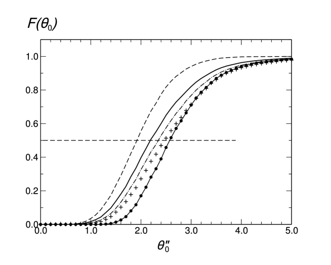
Figure 5: Cumulative isoplanatic angle $\theta_{0}$ distribution for various seasons and conditions: solid line — total scope distribution, dashed – in springs, dot-dashed — falls, crosses — fall 2007, circles — isoplanatic angle when $\beta_{free}$ is better than median.

Equally important for adaptive optics performance, apart from isoplanatic angle, is an atmospheric time constant (widely also called a coherence time) $\tau_{0}$ which is another by-product of scintillation measurement (Tokovinin, 2002). The dedicated study shows that the time constant from MASS estimation is systematically (factor of $\sim 1.3$) lower than observed by other methods. Meanwhile we present uncorrected values hereafter.

Median of $\tau_{0}$ distribution shown in Fig.6 equals to 3.94 ms for the total campaign and 2.82 ms and 4.44 ms for springs and autumns, respectively. When restricted to $\beta_{free}<0\hbox{$.\!\!^{\prime\prime}$}46$ conditions one obtains a 5.41 ms median. If we apply an empiric correction mentioned above, we come to the time constant about 7 ms in good conditions. The latter coincides with the median time constant at Antarctic plateau Dome C obtained with MASS device in 2004 (Kenyon et al., 2006).

One can recall the $\tau_{0}=12$ ms estimate of Ehgamberdiev et al (2000) derived during the international astroclimate campaign of 1998 at Maidanak. Meanwhile, this value was based on a relatively short-term scope of measurements.

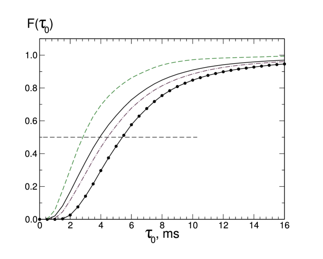
Figure 6: Cumulative distributions of atmospheric coherence time $\tau_{0}$: spring seasons — dotted line, autumns — dash-dotted, full data scope distribution — solid. Black circles depict distribution when $\beta_{free}$ is better than median.

6 PARTICULAR TURBULENCE PROPERTIES OF FREE ATMOSPHERE ABOVE MT. MAIDANAK

In order to study the role of different atmosphere layers, we build the dependence of the relative layers intensity $J_{layer}/J_{total}$ on the total turbulence strength $J_{total}$ according to MASS measurements (i.e. excluding the ground layer). These ratios are shown in Fig. 7 being averaged over 400 profiles. The layer input behavior differs strongly for the boundary layer (0.5 – 1 km) and the upper atmosphere (8 – 16 km). The former shows its input nearly proportional to the total power while the role of the upper atmosphere diminishes with the total growth of turbulence. Most representative here is the 16 km layer for which the relation is practically inversely proportional. This means that its intensity is almost invariable and absolutely insensitive to processes in the boundary layer. Similar phenomenon is noticed by Tokovinin and Travouillon (2006) and in a paper by Thomas-Osip et al (2008).

On the opposite, the boundary turbulence is responsible for image degradation at Maidanak. Keeping in mind the values $J=0.2\times 10^{-12}\mbox{m}^{1/3}$ equivalent to $0\hbox{$.\!\!^{\prime\prime}$}5$ seeing, we are mostly interested in the graph beginnings up to values $0.5\times 10^{-12}\mbox{m}^{1/3}$. At the 2 km height the turbulence intensity is seemingly lower than at other altitudes.

Figure 7: Relative input of atmosphere layers in a total turbulence as a function of latter

As a support for this fact of a key role of the boundary layer, we present the Fig. 8 where the cumulative distributions of layers intensities are shown for a good seeing data subset (image quality better than median). The prominent feature is a nearly absent lower (1 and 2 km) turbulence for 50% of cases. The median of intensity in 4- and 8 km layers is $1.3\div 1.5\times 10^{-14}\mbox{m}^{1/3}$ which is slightly more than the median value for the lowest 0.5 km layer ($1.1\times 10^{-14}\mbox{m}^{1/3}$). It is natural to think that at 0.5 km we see the development of the turbulence generated by a ground relief.

The special case here is again the upper atmosphere at 16 km. The steep rise of the cumulative distribution tells about nearly constant turbulence which is quite significant. In half a time its intensity is in a narrow span of $1.5\div 2.8\times 10^{-14}\mbox{m}^{1/3}$. Note that the high altitude turbulence is restored with a minimal error from the scintillation data.

Figure 8: Cumulative distribution of turbulence intensity in 0.5 km layer (solid line), at 1 km (short dashes), 2 km (long dashes), 4 km (dots), 8 km (short dash-dots) and 16 km (long dash-dots) for cases of good images ($\beta_{free}<0\hbox{$.\!\!^{\prime\prime}$}46$).

7 CONCLUSIONS

An estimation of a total turbulence power from DIMM measurements (Ilyasov et al., 1999) allows us to evaluate the dominating input of the ground turbulence (up to 500 m above surface) to be 65% on average and the first 200 – 300 m above surface give already about 50% contribution. The same contribution is found at Cerro Pachon by Tokovinin and Travouillon (2006).

In cases of exceptionally good images (25% quantile) the full image quality from DIMM measurements in 1996 to 1999 (Ehgamberdiev et al., 2000) constitutes $0\hbox{$.\!\!^{\prime\prime}$}55$. Comparing with data in Fig. 4 we come to the ground layer contribution of 60% in these conditions while the whole boundary layer inputs more than 70% leaving less than one third of a power to the rest of atmosphere.

In such a situation the development of an adaptive optics system working in the visible should be directed to correction of the low turbulence. It is hardly possible to achieve the Strehl ratio improvement factor more than 5 here, meanwhile the large corrected AO field of view (of the order of several arc-minutes, see Rigaut, 2002) will be a reasonable compensation. It is worth to note here that the maximum gain for the median Maidanak conditions (Fried radius $r_{0}=0.15\mbox{m}$ at wavelength 500 nm) at the 1.5 m telescope AZT-22 computed according to Roddier formula (1998) for optimal atmospheric distortions correction is equal to 32.

A profiting advantage of Maidanak observatory is a large time constant value $\tau_{0}\approx 7\mbox{ms}$. This lowers the critical demand of a system response time by a factor of nearly 2.5 and thus makes about three times more stars available for wavefront referencing compared to Cerro Tololo and Cerro Pachon observatories (Kenyon et al., 2006). Such a good $\tau_{0}$ also favours the development of optical interferometry at this site.

This research was supported by Russian Basic Research Foundation (grant 06-02-16902a). The staff of Maidanak observatory helped a lot in organization and conduction of measurements for which we express gratitude to all of them.

References

- Azouit & Vernin (1980) Azouit M., Vernin J., J. Atmos. Sci. 37, 1550 (1980).
- Dravins et al. (1997) Dravins D., Lindegren L., Mezey E., et al., PASP 109, 173 (1997).
- Ehgamberdiev et al. (2000) Ehgamberdiev S.A., Baijumanov A.K., Ilyasov S.P., et al., Astrophys. Space Sci. 145, 293 (2000).
- Fuchs et al. (1998) Fuchs A., Tallon M., and Vernin J., PASP 110, 86 (1998).
- Fuensalida et al. (2004) Fuensalida J., Chueca S., Delgado J.M., et al., Second Backaskog Workshop on Extremely Large Telescopes (Ed. A.L. Ardeberg, T. Andersen, Proc. of the SPIE, 5382, 2004), p. 619.
- Fuensalida et al. (2007) Fuensalida J.J., Garcia-Lorenzo B., Delgado J.M., et al., Workshop on Astronomical Site Evaluation (Ed. I. Cruz-Gonzalez, J. Echevarria, D. Hiriart, Rev. Mexicana de Astronomia y Astrofisica (Serie de Conferencias) 31, 2007), p. 86.
- Ilyasov et al. (1999) Il’yasov S.P., Baizhumanov A.K., Sarazin M., et al., Astronomy Letters 25, 122 (1999).
- Kenyon et al. (2006) Kenyon S.L., Lawrence J.S., Ashley M.C.B., et al., PASP 118, 924 (2006).
- Kornilov & Tokovinin (2001) Kornilov V., Tokovinin A., Astronomy Reports 45, 395 (2001).
- Kornilov et al. (2003) Kornilov V., Tokovinin A., Vozyakova O., et al., Adaptive Optical System Technologies II. (Ed. Wizinowich, P.L., Bonaccini, D., Proc. of SPIE 4839, 2003), p. 837.
- Kornilov et al. (2007) Kornilov V., Tokovinin A., Shatsky N., et al., MNRAS 382, 1268 (2007).
- Rigaut (2002) Rigaut F., Beyond conventional adaptive optics. ESO Topical Meeting (Ed. E. Vernet, R. Ragazzoni, N. Hubin, S. Esposito, Garching: ESO Conf. and Workshop Proc. 58, 2002), p. 11.
- Roddier (1981) Roddier F., Progress in Optics. (Amsterdam: North-Holland Publishing Co., 19, 1981), p. 281
- Roddier (1998) Roddier F., PASP 110, 837 (1998).
- Roddier (1999) Roddier F., Adaptive optics in astronomy, (Ed. F. Roddier, Cambridge, NY, Cambridge University Press, 1999).
- Sadibekova et al. (2006) Sadibekova T., Vernin J., Sarazin M., et al., Ground-based and Airborne Telescopes (Ed. L.M. Stepp, Proc. of the SPIE, 6267, 2006), p. 55.
- Sarazin & Roddier (1990) Sarazin M. and Roddier F., Astron. Astrophys. 227, 294 (1990).
- Shao & Colavita (1992) Shao M. and Colavita M.M., Astron. Astrophys. 262, 353 (1992).
- Tatarskiy (1967) Tatarskiy V.I., Waves propagation in turbulent media [in Russian] Moscow, Nauka, 1967.
- Thomas-Osip et al. (2008) Thomas-Osip J.E., Prieto G., Johns M., and Phillips M.M., Ground-based and Airborne Telescopes (Ed. L.M. Stepp, R. Gilmozzi, Proc. of the SPIE, 7012, 2008), p. 64.
- Tokovinin (1998) Tokovinin A., Astronomy Letters 24, 662 (1998).
- Tokovinin (2002) Tokovinin A., Appl. Optics 41, 957 (2002).
- Tokovinin & Kornilov (2002) Tokovinin A. and Kornilov V., Astronomical Site Evaluation in the Visible and Radio Range, (Ed. J. Vernin, Z. Benkhaldoun, and C. Muñoz-Tuñón, ASP Conf. Series 266, 2002), p.104.
- Tokovinin & Kornilov (2007) Tokovinin A. and Kornilov V., MNRAS 381, 1179 (2007).
- Tokovinin & Travouillon (2006) Tokovinin A. and Travouillon T., MNRAS 365, 1235 (2006).
- Tokovinin et al. (2003a) Tokovinin A., Baumont S., and Vasquez J., MNRAS 340, 52 (2003).
- Tokovinin et al. (2003b) Tokovinin A., Kornilov V., Shatsky N., et al., MNRAS 343, 891 (2003).
- Vernin et al. (1991) Vernin J., Caccia J.-L., Weigelt G., et al., Astron. Astrophys. 243, 553 (1991).
- Wilson et al. (2003) Wilson R.W., Wooder N.J., Rigal F., et al., MNRAS 339, 491 (2003).