Influence of inner and outer walls electromagnetic properties on the onset of a stationary dynamo.

Abstract

To study the onset of a stationary dynamo in the presence of inner or outer walls of various electromagnetic properties, we propose a simple 1D-model in which the flow is replaced by an alpha effect. The equation of dispersion of the problem is derived analytically. It is solved numerically for walls of different thicknesses and of electric conductivity and magnetic permeability different from those of the fluid in motion. We also consider walls in the limit of infinite conductivity or permeability.

1 Introduction

A number of experimental devices have been built in the last years aiming at producing dynamo action (for reviews see e.g. Gailitis02 and Radler02 ). Such a device is generally made of a container in which some liquid metal is put into motion. In a previous study Avalos03 we considered the influence of the electromagnetic properties of the container outer wall onto the onset of dynamo action for the Riga (Latvia) and Karlsruhe (Germany) experiments. The results depend on which type of dynamo instability is obtained. For stationary solutions like in the Karlsruhe experiment Stieglitz01 Muller04 , the reduction of the dynamo instability threshold is monotonic versus the conductivity and the permeability of the outer wall. For oscillatory solutions like in the Riga experiment Gailitis00 Gailitis01 , there are additional eddy currents in the outer wall. These currents produce an additional dissipation opposed to the reduction of the threshold. In that case, the reduction of the dynamo instability threshold versus the conductivity and the permeability of the outer wall is not monotonic anymore.
These results are consistent with other studies aiming at studying the influence of the thickness of a stagnant outer layer conducting fluid (or equivalently of an outer wall with the same conductivity as the fluid) on the dynamo threshold. Various inner flow geometries have been considered leading to either stationary Ravelet05 Sarson96 or oscillatory Kaiser99 Frick02 solutions. In Fig. 1 we give a synthesis of these results. For that we plot the threshold reduction rate $\Gamma$ versus $e/R$ where $\Gamma=1-R_{m}(e/R)/R_{m}(0)$, $e$ is the thickness of the stagnant outer layer, $R$ the radius of the fluid container and $R_{m}$ the magnetic Reynolds number defined by $R_{m}=UR/\eta$ where $U$ is a characteristic flow intensity and $\eta$ the magnetic diffusivity. The stationary solutions correspond to the full curves (a-d) and are increasing monotonically versus $e/R$. The non-stationary solutions correspond to the dashed curves (e-i) and reach a maximum versus $e/R$ (though not obvious for the curves (f) and (h) it is actually the case). The influence of the electric conductivity of an inner core has also been investigated Schubert01 . Again the same conclusions as Avalos03 have been found: for stationary (resp. oscillating) solutions, the dynamo threshold decreases monotonically (resp. reaches a minimum) when increasing the conductivity of the inner core.

$\Gamma$
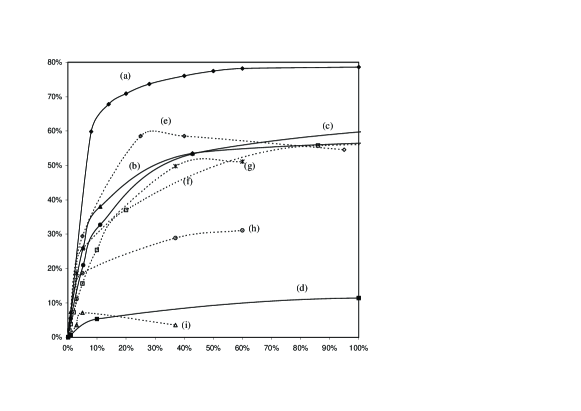
	$e/R$

Figure 1: Threshold reduction rate $\Gamma$ versus $e/R$ for (a) the Von Karman sodium experiment Ravelet05 , the Kumar and Roberts flow for (b) $R_{m}>0$ and (c) $R_{m}<0$ Sarson96 , (d) the Karlsruhe experiment Avalos03 , (e) the Perm experiment Frick02 , (f) the Riga experiment Avalos03 , the s1t1 flow with $\epsilon=$ (g) 0.35, (h) 0.3, (i) 0.25 Kaiser99 .

Given the high difficulties to build a dynamo experiment, reducing the threshold by changing the electromagnetic boundary conditions is of course of high interest for the experimenter. The influence of electromagnetic boundary conditions onto dynamo action has also been the object of different studies relevant to planets, and stars. In the case of Earth-like planets for example, the influence of a conducting solid inner core onto the dynamo action produced by the outer core fluid motion has been studied by different ways, using either a prescribed $\alpha^{2}$-effect Schubert01 , a prescribed $\alpha$-effect and buoyancy Hollerbach95 or a direct resolution of the full convective dynamo model Wicht02 . The main issue of these studies was to identify whether the inner core has a stabilizing effect on the reversals of the dipole component of the magnetic field. So far there is no definite answer to this problem as these different studies lead to contradictory results. In the case of Solar-like stars, it has been shown Thelen00 how some magnetic features (like the PDF of the magnetic field strength) observed at the surface of the star could give some indications on the relevant magnetic boundary conditions of a turbulent convective dynamo model.
Magnetic boundary conditions may also be important in the case of Fast Breeder Reactors (FBR). Indeed, though these industrial installations have not being designed to produce dynamo action, they share some common features with the Karlsruhe experiment. In the core of a FBR, the liquid sodium flows in an array of a large number of parallel straight tubes called assemblies. In each of them the flow geometry is again composed of a periodic array of single helical vortices. One has shown Plunian99 the existence of an $\alpha$-effect similar to the Karlsruhe experiment in each assembly. Though such an $\alpha$-effect is not sufficient to generate a dynamo instability for a core with homogeneous electromagnetic properties, the question remains when the walls of the assemblies are made, for example, of ferromagnetic steel (relative permeability of the order $10^{3}$ and relative conductivity of order 1) Soto99 and when the array of assemblies is surrounded by a belt of ferromagnetic material (as it is the case in the FBR Phenix). In that case both inner and outer walls electromagnetic properties may be important. Indeed a reduction of the dynamo threshold leading to some dynamo instability within the core of the FBR could imped the right working of the reactor and lead for example to an emergency breakdown.

In the present paper we consider a simple 1D-model of a stationary dynamo in order to evaluate the relative importance of inner and outer wall electromagnetic properties onto the onset of dynamo action. For that we consider two types of boundary conditions: either an outer wall and isolating medium outside or periodic inner walls. In both cases we not only vary the relative conductivity and permeability of the walls but also their thicknesses.

2 A simple 1D-model

2.1 An anisotropic $\alpha$-effect

We use the kinematic approach consisting in solving the induction equation for a given motion. This equation reads

$$\frac{\partial\boldsymbol{\rm B}}{\partial t}=\nabla\times(\boldsymbol{\rm U}\times\boldsymbol{\rm B})+\eta\nabla^{2}\boldsymbol{\rm B},\;\;\;\;\nabla.\boldsymbol{\rm B}=0,$$ (1)

where, again, $\eta$ means the magnetic diffusivity of the fluid, $\boldsymbol{\rm B}$ the magnetic field and $\boldsymbol{\rm U}$ the fluid velocity.
As we are not interested by a flow geometry in particular but only by the influence of the boundary conditions onto the onset of dynamo action, we assume that the interactions of the flow with the magnetic field can be represented by an anisotropic $\alpha$-effect like in the Karlsruhe experiment Plunian02 Radler02b or in the core of a FBR Plunian99 . Following the lines of mean–field dynamo theory Krause80 the magnetic field $\boldsymbol{\rm B}$ and the fluid velocity $\boldsymbol{\rm U}$ are expressed as sums of mean fields, $\overline{\boldsymbol{\rm B}}$ and $\overline{\boldsymbol{\rm U}}$, and fluctuating fields, $\boldsymbol{\rm B}^{\prime}$ and $\boldsymbol{\rm U}^{\prime}$. Here the mean is defined by a space average of the original field. Assuming $\overline{\boldsymbol{\rm U}}$ = 0, the mean part of the induction equation (1) writes

$$\frac{\partial\overline{\boldsymbol{\rm B}}}{\partial t}=\nabla\times{\cal E}+\eta\nabla^{2}\overline{\boldsymbol{\rm B}},\;\;\,\,\,\,\;\;\,\,\,\,\nabla.\overline{\boldsymbol{\rm B}}=0,$$ (2)

where ${\cal E}$ is a mean electromotive force due to the fluid motion given by

$${\cal E}=\overline{\boldsymbol{\rm U}^{\prime}\times\boldsymbol{\rm B}^{\prime}}.$$ (3)

We may consider ${\cal E}$ as a functional of $\boldsymbol{\rm U}^{\prime}$ and $\overline{\boldsymbol{\rm B}}$. Let us accept the assumption usually adopted in the mean-field context that ${\cal E}$ in a given point in space and time depends on $\overline{\boldsymbol{\rm B}}$ only via the components of $\overline{\boldsymbol{\rm B}}$ and their first spatial derivatives in this point. This is reasonable for sufficiently small variations of $\overline{\boldsymbol{\rm B}}$ in space and time. For a first approximation, on which we restrict ourselves here, we consider no other contributions to ${\cal E}$ than that describing the $\alpha$-effect, that is, we ignore all contributions to ${\cal E}$ containing derivatives of $\overline{\boldsymbol{\rm B}}$. In addition, the $\alpha$-effect is assumed to act in the $xy$-plane only, where $x$, $y$ and $z$ are the Cartesian coordinates. This corresponds to a flow for example independent of $z$. Then (2) writes in the form

$$\frac{\partial\overline{\boldsymbol{\rm B}}}{\partial t}=-\nabla\times[\alpha(\overline{\boldsymbol{\rm B}}-(\hat{\boldsymbol{\rm z}}.\overline{\boldsymbol{\rm B}})\hat{\boldsymbol{\rm z}})]+\eta\nabla^{2}\overline{\boldsymbol{\rm B}},\;\;\,\,\,\,\nabla.\overline{\boldsymbol{\rm B}}=0$$ (4)

where $\alpha$ is a scalar quantity. Such a model has proved to be sufficiently realistic for both cases, the Karlsruhe experiment Plunian02 Radler02b and the FBR core Plunian99 . However for the latter case, there is an additional mean flow $\overline{\boldsymbol{\rm U}}$ along the $z$-direction which affects the model. The corresponding discussion is postponed to section 5.

2.2 Model parameters

We consider three regions $l$ (=1, 2 or 3) symmetric with respect to the plane $x=0$ and infinite in the $y$ and $z$ directions. They are defined by their respective size along $x$ ($\pm x\leq R$, $R\leq\pm x\leq R+e$ and $\pm x\geq R+e$), conductivity ($\sigma_{1}$, $\sigma_{2}$, $\sigma_{3}$), permeability ($\mu_{1}$, $\mu_{2}$, $\mu_{3}$) and $\alpha$-effect ($\alpha_{1}=\alpha$, $\alpha_{2}=0$, $\alpha_{3}=0$) where $\alpha$ is a steady scalar quantity which does not depend on $x$, $y$ nor $z$.
We also consider two types of boundary conditions in the $x$-direction (see Fig. 2). The problem in which the region 3 is an insulator ($\sigma_{3}=0$) and extends to infinity with $\overline{\boldsymbol{\rm B}}(x)\rightarrow 0$ when $x\rightarrow\infty$ is called the non-periodic problem. In that case the region 2 corresponds to an outer wall. The problem in which the region 3 does not exists and $\overline{\boldsymbol{\rm B}}(x=R+e)=\overline{\boldsymbol{\rm B}}(x=-R-e)$ is called the periodic problem. In that case the region 2 corresponds to periodic inner walls like the walls of the assemblies of a FBR.

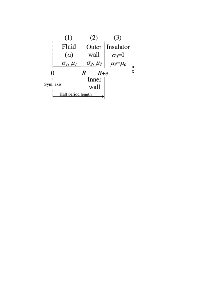
Figure 2: Scheme of the 3 regions of the non periodic problem (above) and of the 2 regions of the periodic problem (below).

2.3 Reduction of the basic equations

The solutions of (4) can be represented as series of Fourier modes proportional to $\exp(ijy+ikz)$. As $\alpha$ does not depend neither on $y$ nor $z$, each ($j,k$)-mode is independent from each other. As $\alpha$ is steady we may expect solutions varying like $\exp(pt)$ in time, with the real part of $p$ being the growth rate of the magnetic field. In the rest of the paper we consider only the mode $j=0$, for sake of simplicity. Then, for a given $k$, we may look for $\overline{\boldsymbol{\rm B}}$ in the form

$$\overline{\boldsymbol{\rm B}}=\Re[\boldsymbol{\rm b}(x)\exp(pt+ikz)]\;\;\;\mbox{with}\;\;\;\boldsymbol{\rm b}=(-ika,b,\partial_{x}a),$$ (5)

$a$ and $b$ being functions of $x$ only. Replacing (5) in (4), we find the following equations

$$(\eta_{l}\Delta-p)a_{l}-\alpha_{l}b_{l}=0$$ (6)

$$(\eta_{l}\Delta-p)b_{l}-\alpha_{l}k^{2}a_{l}=0$$ (7)

where $\eta_{l}=1/\sigma_{l}\mu_{l}$, $\Delta=\partial_{x^{2}}-k^{2}$ and $l=1,2,3$ ($l=1,2$) for the non-periodic (periodic) problem.
We can show that there exists two sets of independent solutions depending on the parity of $a_{1}(x)$ and $b_{1}(x)$. Indeed, from (6) and (7) $a_{1}$ is solution of $L(a_{1})=0$ with $L=(\eta_{1}\Delta-p)^{2}-\alpha^{2}k^{2}$. This operator $L$ is linear and leaves the parity of the function unchanged. Therefore writing $a_{1}$ as the sum of an odd and even functions $a_{1}=a_{1}^{o}+a_{1}^{e}$ we find that $L(a_{1}^{o})=L(a_{1}^{e})=0$. Consequently, $a_{1}^{o}$ and $a_{1}^{e}$ are two independent solutions of $L$. From (6) and (7), it is easy to show that $b_{1}$ has the same parity as $a_{1}$. Therefore it is sufficient to solve (6) and (7) for each parity, the general solution being a linear combination of them. The solution at $x=0$ is given by $\boldsymbol{\rm b}=(0,0,b_{z})$ if $a_{1}(x)$ is odd and $\boldsymbol{\rm b}=(0,b_{y},b_{z})$ if $a_{1}(x)$ is even.

3 Method of resolution

3.1 General solutions

The general form of the solutions of equations (6) and (7) write:

$$a_{1} = \frac{1}{k}(A_{1c}^{+}\cosh\omega_{1}^{+}x+A_{1c}^{-}\cosh\omega_{1}^{-}x$$

$$+\;\;A_{1s}^{+}\sinh\omega_{1}^{+}x+A_{1s}^{-}\sinh\omega_{1}^{-}x)$$

$$b_{1} = B_{1c}^{+}\cosh\omega_{1}^{+}x+B_{1c}^{-}\cosh\omega_{1}^{-}x$$ (8)

$$+ B_{1s}^{+}\sinh\omega_{1}^{+}x+B_{1s}^{-}\sinh\omega_{1}^{-}x$$

$$a_{2} = \frac{1}{k}(A_{2c}\cosh\omega_{2}x+A_{2s}\sinh\omega_{2}x)$$

$$b_{2} = B_{2c}\cosh\omega_{2}x+B_{2s}\sinh\omega_{2}x$$

$$a_{3} = \frac{A_{3}}{k}\exp(-\omega_{3}x)$$

$$b_{3} = B_{3}\exp(-\omega_{3}x)$$

with

$$(\omega_{1}^{\pm})^{2} = k^{2}+\frac{p\pm\alpha k}{\eta_{1}},\;\;(\omega_{2})^{2}=k^{2}+\frac{p}{\eta_{2}},$$ (9)

$$(\omega_{3})^{2} = k^{2}+\frac{p}{\eta_{3}}\;\;\;\mbox{and}\;\;\;\Re(\omega_{3})>0$$

and where $a_{3}$ and $b_{3}$ are the solutions in the region 3 for the non periodic problem only. In that case we applied the condition $\boldsymbol{\rm b}_{3}\rightarrow 0$ when $r\rightarrow\infty$. Furthermore, for sake of generality, we shall replace $\sigma_{3}$ by 0 only in the numerical applications.
Applying the appropriate symmetry conditions in $x=0$, the following relations are found for the even solutions:

$$A_{1s}^{+}=A_{1s}^{-}=B_{1s}^{+}=B_{1s}^{-}=0.$$ (10)

From (6) we have the additional relations:

$$A_{1c}^{+}=B_{1c}^{+},\;\;\;\;\;A_{1c}^{-}=-B_{1c}^{-}$$ (11)

for both problems non-periodic and periodic. For the even solutions of the periodic problem the boundary condition $\boldsymbol{\rm b}_{2}(R+2e)=\boldsymbol{\rm b}_{2}(R)$ leads to the additional relations

$$A_{2c}\sinh\omega_{2}(R+e) = -A_{2s}\cosh\omega_{2}(R+e)$$

$$B_{2c}\sinh\omega_{2}(R+e) = -B_{2s}\cosh\omega_{2}(R+e).$$ (12)

For the odd solutions the same relations as (10) and (11) are found with inverted subscripts $s$ and $c$. For the odd solutions of the periodic problem the boundary conditions $\boldsymbol{\rm b}_{2}(R+2e)=-\boldsymbol{\rm b}_{2}(R)$ leads to the additional relations given by (12) with, again, inverted subscripts $s$ and $c$.

3.2 Boundary conditions

The normal component of $\overline{\boldsymbol{\rm B}}$, the tangential component of $\overline{\boldsymbol{\rm B}}/\mu$ and the $z$-component of the electric field $E_{z}=\eta(\nabla\times\overline{\boldsymbol{\rm B}})_{z}$ are continuous across each interface $x=R$ and $x=R+e$. We can show that this set of relations is sufficient to describe all the boundary conditions of the problem. They write for $l$=1, 2 ($l=1$) corresponding to the non-periodic (periodic) case:

$$a_{l}(x=x_{l}) = a_{l+1}(x=x_{l})$$

$$\frac{1}{\mu_{l}}b_{l}(x=x_{l}) = \frac{1}{\mu_{l+1}}b_{l+1}(x=x_{l})$$

$$\frac{1}{\mu_{l}}a^{\prime}_{l}(x=x_{l}) = \frac{1}{\mu_{l+1}}a^{\prime}_{l+1}(x=x_{l})$$

$$\eta_{l}b^{\prime}_{l}(x=x_{l}) = \eta_{l+1}b^{\prime}_{l+1}(x=x_{l})$$ (13)

where the prime denotes the $x$-derivative, $x_{1}=R$ and $x_{2}=R+e$.

3.3 Resolution

Replacing (8) into (13) and applying (10), (11) and (12), we find a system to solve. The solution is non trivial only if the determinant of the system is equal to zero. This determinant writes

$$1+\frac{M+S}{2}(X_{1}^{+}+X_{1}^{-})+MSX_{1}^{+}X_{1}^{-}=0$$ (14)

with $X_{1}^{\pm}=R\omega_{1}^{\pm}\tanh R\omega_{1}^{\pm}$ for the even solutions and $X_{1}^{\pm}=R\omega_{1}^{\pm}\coth R\omega_{1}^{\pm}$ for the odd solutions.
For both even and odd solutions of the non-periodic problem, $M$ and $S$ are defined by

$$M=\frac{m}{R\omega_{2}}\frac{1+\frac{n\omega_{3}}{\omega_{2}}\tanh e\omega_{2}}{\frac{n\omega_{3}}{\omega_{2}}+\tanh e\omega_{2}}\;,\;\;S=\frac{s}{R\omega_{2}}\frac{1+\frac{r\omega_{3}}{\omega_{2}}\tanh e\omega_{2}}{\frac{r\omega_{3}}{\omega_{2}}+\tanh e\omega_{2}}.$$ (15)

For the periodic problem, $M$ and $S$ are defined by

$$(M,S) = (m,s)\frac{\coth e\omega_{2}}{R\omega_{2}}\;\;\;\;\;\;\mbox{for even solutions,}$$ (16)

$$(M,S) = (m,s)\frac{\tanh e\omega_{2}}{R\omega_{2}}\;\;\;\;\;\;\mbox{for odd solutions,}$$ (17)

with

$$m=\frac{\mu_{2}}{\mu_{1}},\;\;\;n=\frac{\mu_{2}}{\mu_{3}},\;\;\;s=\frac{\sigma_{2}}{\sigma_{1}},\;\;\;r=\frac{\sigma_{2}}{\sigma_{3}}.$$ (18)

4 Results

4.1 General remarks

We can show that the growth rate $p$ has no imaginary part as shown in Appendix A. An additional and simple argument is that, as the $\alpha$-effect does not depend on $z$, there is no preferred way along the $z$-direction for a magnetic wave to travel. Therefore, the marginal instability solution corresponds to $p=0$. This leads to $\omega_{2}=\omega_{3}=k$.
The results are given in terms of the dimensionless quantities $m$, $n$, $s$, $r$ defined in (18) and of $\hat{k}=kR$, $\hat{p}=pR^{2}/\eta_{1}$, $\hat{\omega_{l}}=R\omega_{l}$, $\hat{e}=e/R$ and $R_{\alpha}=R\alpha/\eta_{1}$. The hat is dropped in the rest of the paper for sake of clarity. Then for a given set of the parameters $m,n,s,r,k,e$ we seek solutions such that $p=0$ and $R_{\alpha}$ is minimum.
From (9) we see that replacing $R_{\alpha}$ by -$R_{\alpha}$ is the same as replacing $k$ by $-k$ and also the same as replacing $\omega_{1}^{+}$ by $\omega_{1}^{-}$. As (14) is symmetric in $\omega_{1}^{+}$ and $\omega_{1}^{-}$, it is then sufficient to consider only positive values of $k$ and $R_{\alpha}$.
For the non-periodic problem we set $\sigma_{3}=0$ (the region 3 being insulating). This corresponds to the limit $r\rightarrow\infty$ . It leaves (14) unchanged but $\omega_{3}=k$ and $S=s\frac{\tanh\omega_{2}e}{\omega_{2}}$.

4.2 Influence of wall thickness

In Fig. 3 the marginal curves $\log_{10}(R_{\alpha})$ versus $\log_{10}(k)$ are given for $s=10$, $m=n=1$ and different values of $e$. The marginal curves of the odd solutions are located between the curves (d) and (e) and therefore always above the marginal curves of the even solutions located between the curves (a) and (c). Therefore only the even solutions are present at the onset of the dynamo action unless $k$ is large. The same comments apply when varying $s$, $m$ or $n$. Therefore in the subsequent subsections we shall focus only on the even solutions.
The marginal curves of the non-periodic problem are located between the curves (c) and (b). They are always above those of the periodic problem located between the curves (a) and (b). Then the periodic problem appears to be always more unstable than the non-periodic problem. However in the limit of large $ke$ both problems have the same marginal curve (b). Indeed taking $ke>>1$ in (15) and (16) leads to $(M,S)=(m,s)/k$ for both problems. Also taking $ke>>1$ means that the fluid is embedded between walls of infinite thickness (compared to the vertical wave length of the field). Then no distinction can be found between both problems. From asymptotic estimates, we can show that

$$\lim_{ke\rightarrow\infty,k\rightarrow 0}R_{\alpha}=(ms)^{-1/2}$$ (19)

which corresponds to the asymptotic left part of the curve (b).
The curve (a) is obtained for $e=0$ for the periodic problem (even solutions). We can show that it is given by

$$R_{\alpha}=k.$$ (20)

which has already been obtained in other periodic problems (without walls) in which an anisotropic $\alpha$-effect is the dynamo mechanism (see e.g. Plunian99 Plunian02 ).
The curve (c) is obtained for $e=0$ for the non-periodic problem (even solutions). From asymptotic estimate we can show that for $k<<1$ it is given by

$$R_{\alpha}=\sqrt{3n/mk}.$$ (21)

In the limit of small or large values of both $k$ and $ke$, asymptotic expansions in $k$ of $R_{\alpha}$ have been calculated. A synthesis of these expansions is given in table 1.

	$R_{\alpha}$	$k<<1$ and $ke<<1$	$k>>1$ and $ke>>1$
even	n.p.	$\sqrt{\frac{n/m}{se+1/3}}\frac{1}{\sqrt{k}}+\frac{1}{\sqrt{k}}O(1)$	$k+(\frac{\pi}{2})^{2}\frac{1}{k}-$
	per.	$\sqrt{(1+e/m)(1+e/s)}\;k+O(k)$	$(\frac{\pi}{2})^{2}\sqrt{2}\frac{m+s+2\sqrt{2}ms}{m+s+\sqrt{2}}\frac{1}{k^{2}}+O(\frac{1}{k^{2}})$
odd		$\frac{c^{2}}{k}+\frac{1}{k}O(1)$	$k+\pi^{2}(\frac{1}{k}-\sqrt{2}\frac{m+s+2\sqrt{2}ms}{m+s+\sqrt{2}}\frac{1}{k^{2}})+O(\frac{1}{k^{2}})$

Table 1: Asymptotic expansion in $k$ of $R_{\alpha}$ for both problems non-periodic and periodic. The parameter $c$ ($\frac{\pi}{2}<c<\pi$) is solution of the equation $\frac{1}{2se}(\tan c+\tanh c)=-c$ for the non-periodic problem and $(\frac{m+s}{2}+msec\cot c)(\frac{m+s}{2}+msec\coth c)=(\frac{m-s}{2})^{2}$ for the periodic problem.

These expansions fit very well to the slopes of the curves of Fig. 3.

$\log_{10}(R_{\alpha})$
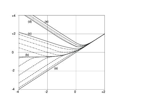
	$\log_{10}(k)$

Figure 3: The marginal curves $\log_{10}(R_{\alpha})$ versus $\log_{10}(k)$ for $m=n=1$, $s=10$ and different values of $e$. The dashed curves between (a) and (b) correspond to the periodic even solutions. From (a) to (b): $e$=0 (curve (a)),$e=1,10,10^{2},10^{3},10^{4}$ and $e\rightarrow\infty$ (curve (b)). The dotted-dashed curves between (b) and (c) correspond to the non-periodic even solutions. From (c) to (b): $e$=0 (curve (c)),$e=0.1,1,10,10^{2}$ and $e\rightarrow\infty$ (curve (b)). The dotted curves between (d) and (e) correspond to the odd solutions for both problems (periodic and non-periodic). They are obtained respectively in the limit of large $e$ (curve (d)) and for $e=0$ (curve (e)).

In the limit of small $ke$ and large $e$ these expansions also give $R_{\alpha}=O(e^{-1/2})$ for the non-periodic and $R_{\alpha}=O(e)$ for the periodic even solutions. Then for increasing $e$, the non-periodic problem gets more unstable whereas the periodic problem gets more stable. To get a qualitative explanation to this striking difference between both problems, we sketch in Fig. 4 the dimensionless dissipation rate $\cal{J}$ (ratio of the Joule dissipation to the magnetic energy, see details in Appendix B) versus $e$. We also sketch on the same figure the dimensionless rate of the work of the Lorentz forces $\cal{S}$. Then $R_{\alpha}$ is defined by $R_{\alpha}=\cal{J}/\cal{S}$.

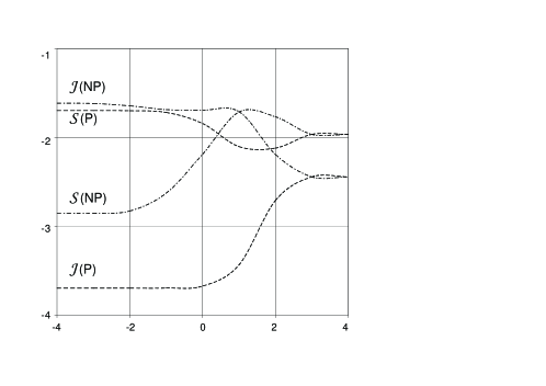
	$\log_{10}(e)$

Figure 4: Dissipation rate $\cal{J}$ and work of the Lorentz forces rate $\cal{S}$ versus $\log_{10}(e)$ for $m=n=1$, $s=10$ and $k=0.01$ for both problems periodic (P) and non-periodic (NP).

What is remarkable is that the decrease (increase) of $R_{\alpha}$ for the non-periodic (periodic) problem is not only due to a decrease (increase) of $\cal{J}$ but also to an increase (decrease) of $\cal{S}$. We also find that the dissipation in the wall in both cases is always negligible compared to the dissipation in the fluid. This shows that changing $e$ leads to a pure geometrical effect on the field and current lines, a consequence of it being the change of the dissipation in the fluid and work of the Lorentz forces. As an illustration we sketch in Fig.5 the isolines of $\Re[b(x)\exp(ikz)]$ for different values of $e$. These isolines correspond to the current density lines in the $(x,z)$-plane and also to the isolines of the $y$-component of the magnetic field. We see that increasing the thickness (from left to right) for both problems periodic (top) and non-periodic (bottom) changes indeed the geometry of these isolines. Increasing $e$ leads to a bending (flattening) of the current lines for the periodic (non-periodic) problem, enhancing (decreasing) Joule dissipation, consistently with Fig.4.

(a)	(b)	(c)	(d)
(e)	(f)	(g)	(h)

Figure 5: Isolines of $\Re[b(x)\exp(ikz)]$ in the $(x,z)$-plane ($0\leq x\leq 1$) for $m=n=1$, $s=10$, $k=0.01$, for both periodic ($0\leq kz\leq\pi/100$) and non-periodic ($0\leq kz\leq\pi$) problems and different values of $e$. The isolines of the periodic problem are given for (a) $e=10^{-1}$, (b) $e=1$, (c) $e=10$ and (d) $e=10^{2}$. The isolines of the non-periodic problem are given for (e) $e=0$, (f) $e=10^{-2}$, (g) $e=10^{-1}$ and (h) $e=1$.

4.3 Influence of wall conductivity and permeability

The expansions of table 1 for small values of both $k$ and $ke$ also give the dependency of $R_{\alpha}$ versus $m$ and $s$. For large (resp. small) value of $m$ and $s$, $R_{\alpha}=O((ms)^{-1/2})$ for the non-periodic (resp. periodic) even solutions. This means that the dynamo onset is easier to reach with walls of higher permeability and/or conductivity. This is true also outside the previous asymptotic limits as depicted in Fig. 6, Fig. 7 and Fig. 8.

$R_{\alpha}$
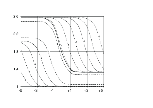
	$\log_{10}(s)$

Figure 6: The marginal curves $R_{\alpha}$ versus $\log_{10}(s)$ for $k=m=n=1$ and different values of $e$. The dashed (dotted-dashed) curves correspond to the periodic (non-periodic) even solutions. The labels indicate $\log_{10}(e)$. The full line is common to both problems in the limit of large $e$.

$R_{\alpha}$
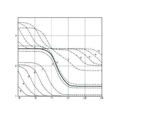
	$\log_{10}(m)$

Figure 7: The marginal curves $R_{\alpha}$ versus $\log_{10}(m)$ for $k=s=1$, $n=m$ and different values of $e$. The dashed (dotted-dashed) curves correspond to the periodic (non-periodic) even solutions. The labels indicate $\log_{10}(e)$. The full line is common to both problems in the limit of large $e$.

$\log_{10}(m)$
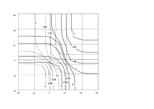
	$\log_{10}(s)$

Figure 8: Isolines of $R_{\alpha}$ in the ($\log_{10}(s)$, $\log_{10}(m)$)-plane for $k=1$, $e=0.1$ and $n=m$. The dashed (full) curves correspond to the periodic (non-periodic) even solutions.

In Fig. 6 the marginal curves $R_{\alpha}$ versus $\log_{10}(s)$ are given for $k=1$, $m=n=1$ and different values of $e$. The dashed (dotted-dashed) curves correspond to the periodic (non-periodic) even solutions. Again, both problems (periodic and non-periodic) have a common solution corresponding to the full curve of Fig. 6 in the limit of large $e$. The monotonic decrease of $R_{\alpha}$ versus $s$ is in agreement with the stationary solutions of Avalos03 for the outer wall problem and of Schubert01 for the inner wall problem.
In Fig. 7 the marginal curves $R_{\alpha}$ versus $\log_{10}(m)$ are given for $k=1$, $s=n=1$ and different values of $e$. The dashed (dotted-dashed) curves correspond to the periodic (non-periodic) even solutions. Again, both problems (periodic and non-periodic) have a common solution corresponding to the full curve of Fig. 7 in the limit of large $e$. This curve coincides with the full curve of Fig. 6. Indeed for a given $k$ and in the limit of large $e$ we find from (15) and (16) that $(M,S)=(m,s)/k$ for both problems. As (14) is symmetric in $M$ and $S$, the full curves of Fig. 6 and Fig. 7 coincide. For the same reason the dashed curves corresponding to the periodic problem of Fig. 6 and Fig. 7 coincide. Again the monotonic decrease of $R_{\alpha}$ versus $m$ is in agreement with the stationary solutions of Avalos03
In Fig. 8 the isolines of $R_{\alpha}$ are sketched in the ($\log_{10}(s)$, $\log_{10}(m)$)-plane for $k=1$, $e=0.1$ and $n=m$. The isolines of the periodic even solutions (dashed curves) are symmetric to the straight line $m=s$ from the same symmetry arguments as above. This is not true for the non-periodic even solutions (full lines). In that case the asymmetry comes from the fact that $\sigma_{3}$ and $\mu_{3}$ do not play a symmetric role as $\sigma_{3}=0$ and $\mu_{3}\neq 0$. In table 2 we give the values of $R_{\alpha}$ for asymptotic values of $(s,m)$. We note that they do not depend on the type of the problem either periodic or non periodic.

	$s<<1$	$s>>1$
$m<<1$	3.5	2.04
$m>>1$	2.03	1

Table 2: Values of $R_{\alpha}$ for asymptotic values of $(s,m)$ and $k=1$, $e=0.1$, $n=m$ and both problems periodic and non periodic.

At that point we can make two conclusions. First in the non periodic case when varying the electromagnetic properties of the outer wall, the roles of the conductivity and permeability are different. In other words, a given jump of magnetic diffusivity $\eta=1/\sigma\mu$ between the fluid and the wall can lead to different results depending on the respective jumps of the conductivity and permeability. Second, for the periodic problem and $e=10^{-1}$, we see from Fig. 7 that when increasing $m$ from $1$ to $10^{3}$ the reduction of the threshold is small ($4.5\%$). Now we see from Fig. 8 that such a reduction at $m=10^{3}$ can be compensated by the decrease of $s$ from 1 to 0.89. In other words the threshold is the same ($\sim$ 1.1) for $(s,m)=(1,1)$ and $(s,m)=(0.89,10^{3})$. Then the reduction of the threshold when using ferromagnetic steel inner walls (with a relative conductivity of order 1) instead of non ferromagnetic materials is negligible. Therefore it does not seem likely that the dynamo action in a FBR can be favored by the use of ferromagnetic assemblies at least in the framework of this simplified study. This is in disagreement with more elaborate models Soto99 which show that the jump of $m$ from 1 to $10^{3}$ reduces the threshold significantly enough to start the dynamo action inside the core of a FBR. A reason of discrepancy may come from the fact that in Soto99 $s$ is kept constant. Also it may come from the idealized geometry of the flow inside each assembly in Soto99 which is helical instead of being replaced by some $\alpha$-effect as here. Now let us consider the influence of a ferromagnetic belt surrounding the core of a FBR. From Fig. 7 we see that, for the non periodic problem, from $m=1$ to $m=10^{3}$ the threshold reduction rate is significant (larger than $20\%$ for $e=10^{-1}$ and $e=1$). If now we assume that the ferromagnetic material is less conducting than the fluid then from Fig. 8 jumping from $(s,m)=(1,1)$ to $s\leq 1$ and $m=10^{3}$ leads to a minimum threshold reduction of $10\%$. Finally it is likely that an outer ferromagnetic belt can favour the dynamo action in the core of a FBR.

4.4 Influence of the fluid permeability

The influence of the fluid permeability can also be given by the expansions of table 1 for small values of both $k$ and $ke$. We see indeed that $R_{\alpha}=O((n/m)^{1/2})$ for the non-periodic even solutions and that $R_{\alpha}=O((1/m)^{1/2})$ in the limit of large $1/m$ for the periodic even solutions. Therefore for both problems a fluid with large permeability leads to higher $R_{\alpha}$. This is also confirmed by Fig.9 in which the marginal curves $R_{\alpha}$ versus $n/m$ are given for $k=1$, $s=n=1$ and different values of $e$. The dashed (dotted-dashed) curves correspond to the periodic (non-periodic) even solutions.

$R_{\alpha}$
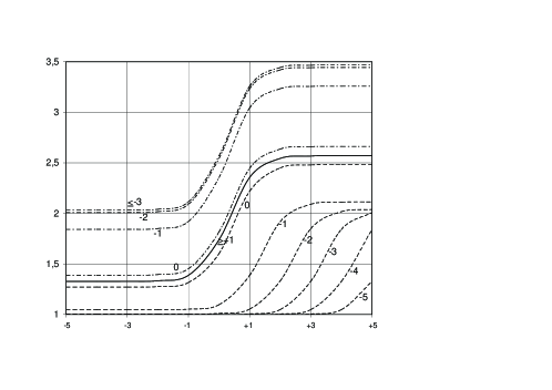
	$\log_{10}(n/m)$

Figure 9: The marginal curves $R_{\alpha}$ versus $\log_{10}(n/m)$ for $k=1$, $s=n=1$ and different values of $e$. The labels indicate $\log_{10}(e)$. The dashed (dotted-dashed) curves correspond to the periodic (non-periodic) even solutions.

Though $R_{\alpha}$ increases versus $n/m$ we must note however that $R_{\alpha}/\sigma_{1}\mu_{1}$ decreases versus $n/m$ (see also Avalos03 ). This means that, keeping $R_{\alpha}$ constant and using a fluid of high permeability allows the experimenter to reduce significantly the flow intensity or the size of the device. Assuming as in Fauve03 that the power to drive an experiment is dissipated by turbulence, leads to a power proportional to $U^{3}$. Therefore using a fluid of high permeability would imply a significant reduction of the driving power. This has also motivated some experimental studies Martin00 Frick02b .

4.5 Geometrical effects

Following the same idea as in section 4.2, we calculate the dissipation and work of the Lorentz force rates for each previous case (changing the conductivity or permeability of the wall or the fluid). We find again that the change of ${\cal J}$ is always accompanied by a change of ${\cal S}$ and that the dissipation in the wall is always negligible compared to the dissipation in the fluid. In table 3, we give some global informations on the behavior of ${\cal J}$ and ${\cal S}$ for the different previous cases. For the same reasons as in section 4.2 we conclude that adding outer or inner walls with different conductivity or permeability has a pure geometrical effect on the field and current lines.

		$e$ $\nearrow$	$s$ $\nearrow$	$m=n$ $\nearrow$	$1/m$ $\nearrow$
Non per.	$\cal S$	$\nearrow$ 7.7	$\nearrow$ 1.17	$\searrow$ 6.22	$\nearrow$ 6.22
	$\cal J$	$\searrow$ 6.76	$\searrow$ 1.65	$\searrow$ 11	$\nearrow$ 11
$R_{\alpha}=$	${\cal J/S}$	$\searrow$ 52	$\searrow$ 1.93	$\searrow$ 1.77	$\nearrow$ 1.77
Periodic	$\cal S$	$\searrow$ 2	$\nearrow$ 1.14	$\searrow$ 1.3	$\nearrow$ 1.3
	$\cal J$	$\nearrow$ 17	$\searrow$ 1.77	$\searrow$ 2.52	$\nearrow$ 2.52
$R_{\alpha}=$	${\cal J/S}$	$\searrow$ 34	$\searrow$ 2	$\searrow$ 1.94	$\nearrow$ 1.94

Table 3: Global information on the evolution of $\cal S$ and $\cal J$ versus $e$ (for $k=0.01$) and versus $s$, $m=n$ and $1/m$ (for $k=1$). The arrows indicate if the quantity grows or decays. The numbers indicate the factor of growth or decay.

4.6 Infinite conductivity or permeability

Two usual ways to simplify the dynamo problem are to solve the induction equation in region 1 only, with one of the following boundary conditions at $x=1$:

$$\boldsymbol{\rm B}\cdot\boldsymbol{\rm n}=\boldsymbol{\rm n}\times\boldsymbol{\rm E}=0,$$ (22)

or

$$\boldsymbol{\rm n}\times\boldsymbol{\rm B}=\boldsymbol{\rm j}\cdot\boldsymbol{\rm n}=0.$$ (23)

The first boundary condition (22) corresponds to region 2 being a perfect conductor whereas the second boundary condition (23) corresponds to region 2 having an infinite permeability. A priori we would expect to recover these two limits with our model taking the limit $s>>1$ or $m>>1$. Furthermore these limits should not depend on $e$ nor on the type of problem periodic or non periodic which is considered. As can be seen from Fig. 6 and Fig. 7 this is not true. In fact it is known Landau69 that considering an ordinary body of electric conductivity $\sigma$ and magnetic permeability $\mu$, the supraconductivity limit corresponds not only to $\sigma\rightarrow\infty$ but in addition to $\mu\rightarrow 0$ . Considering the double limit $s>>1$ and $m<<1$ in our model we indeed recover the boundary condition (22). A body of high permeability is also known to be a poor conductor and corresponds not only to $\mu\rightarrow\infty$ but in addition to $\sigma\rightarrow 0$ . Considering the double limit $m>>1$ and $s<<1$ in our model we indeed recover the boundary condition (23). For both double limits the dynamo threshold is found to be $R_{\alpha}\approx 2$ as given in table 2 .

5 Conclusions

For a stationary dynamo with either insulating or periodic boundary conditions, we showed that additional outer or inner walls change the geometry of the field and current lines in the fluid. This geometrical effect has an effect on the dynamo instability threshold. For given inner or outer walls, increasing their conductivity or permeability helps for dynamo action. In the other hand increasing the thickness of the inner wall plays against the dynamo action (contrary to the outer wall for which increasing the thickness helps for dynamo action). These conclusions are consistent with those obtained in other geometries for outer Avalos03 Ravelet05 Sarson96 as well as inner Schubert01 walls and we believe that they are generic in the sense that they do not depend on the generation process ($\alpha^{2}$ or else) as far as the solution stays stationary. The detailed mechanism of the geometrical effect is however non trivial as the dissipation in the fluid is changed as well as the work of the Lorentz forces. In any case the dissipation in the walls is always negligible.
The usual boundary conditions used to describe a perfectly conducting or high permeability outer wall are recovered with a double limit on $s$ and $m$, stressing that a supraconductor outer wall would correspond to $s\rightarrow\infty$ and $m\rightarrow 0$ and a high permeability outer wall to $m\rightarrow\infty$ and $s\rightarrow 0$.
As mentioned in section 2.1, an additional mean flow $\overline{\boldsymbol{\rm U}}$ like in the core of a fast breeder reactor might lead to oscillatory dynamo solutions. Then in this case as shown in Avalos03 for the Riga dynamo experiment, some additional eddy currents in the walls may lead to significant dissipation in the walls reminiscent to a skin effect. Then the previous behavior of $R_{\alpha}$ versus $e$, $s$ or $m$ would not be monotonic anymore. For the specific case of the core of a FBR, the conclusions of section 4.3 should then be revised with respect to this additional mean flow $\overline{\boldsymbol{\rm U}}$. It is not clear a priori what would be the main effect of $\overline{\boldsymbol{\rm U}}$, either increasing or decreasing the dynamo threshold.

R. Avalos-Zuñiga acknowledges the Mexican CONACYT for financial support.

Appendix A. Proof that $p$ has no imaginary part

Taking (7) and the complex conjugate of (6), we easily find

$$\eta_{l}a_{l}\underline{a}_{l}^{\prime\prime}-(\eta_{l}k^{2}+\underline{p}){|a_{l}|}^{2}-\alpha_{l}\underline{b}_{l}a_{l}=0$$ (A.1)

$$\eta_{l}b_{l}^{\prime\prime}\underline{b}_{l}-(\eta_{l}k^{2}+p){|b_{l}|}^{2}-\alpha_{l}k^{2}\underline{b}_{l}a_{l}=0$$ (A.2)

where an underlined quantity means the complex conjugate of this quantity. Integrating by part and using the boundary conditions (13) we can show that

$$\int_{x_{l-1}}^{x_{l}}a_{l}\underline{a}_{l}^{\prime\prime}dx = -\frac{\mu_{l}}{\mu_{l-1}}a_{l-1}\underline{a}_{l-1}^{\prime}(x_{l-1})+a_{l}\underline{a}_{l}^{\prime}(x_{l})$$ (A.3)

$$- \int_{x_{l-1}}^{x_{l}}|a_{l}^{\prime}|^{2}dx$$

$$\int_{x_{l-1}}^{x_{l}}b_{l}^{\prime\prime}\underline{b}_{l}dx = -\frac{\eta_{l-1}\mu_{l}}{\eta_{l}\mu_{l-1}}b_{l-1}^{\prime}\underline{b}_{l-1}(x_{l-1})+b_{l}^{\prime}\underline{b}_{l}(x_{l})$$ (A.4)

$$- \int_{x_{l-1}}^{x_{l}}|b_{l}^{\prime}|^{2}dx$$

where $x_{0}=a_{0}=b_{0}=0$. For the non-periodic case $x_{3}=+\infty$ and $a_{3}(x=+\infty)=b_{3}(x=+\infty)=0$. For the periodic case the periodicity implies that $a_{2}\underline{a}_{2}^{\prime}(x=R+e)=b^{\prime}_{2}\underline{b}_{2}(x=R+e)=0$. The previous relations do not depend on the parity of $a_{1}$ nor $b_{1}$. Combining the integral of relations (A.1) and (A.2), we find:

$$0=\sum_{l}\frac{1}{\mu_{l}}\int_{x_{l-1}}^{x_{l}}( - \eta_{1}k^{2}|a_{l}^{\prime}|^{2}+\eta_{l}|b_{l}^{\prime}|^{2}-\eta_{1}k^{4}|a_{l}|^{2}$$

$$+ \eta_{l}k^{2}|b_{l}|^{2}-\frac{\eta_{1}}{\eta_{l}}k^{2}\underline{p}|a_{l}|^{2}+p|b_{l}|^{2})dx.$$

Then it is straightforward to show that $\Im(p)=0$.

Appendix B. Expression of the dissipation rate

Multiplying (4) by $\overline{\boldsymbol{\rm B}}/\mu$ we obtain the following equation (where underlying means complex conjugate):

$$\frac{\partial}{\partial t}(\frac{|\boldsymbol{\rm b}|^{2}}{2\mu})=\frac{\partial}{\partial x}(\frac{\underline{\boldsymbol{\rm b}}\times\boldsymbol{\rm e}}{\mu})-\alpha(\boldsymbol{\rm b}-(\hat{\boldsymbol{\rm z}}.\boldsymbol{\rm b})\hat{\boldsymbol{\rm z}})\cdot\underline{\boldsymbol{\rm j}}-\frac{|\boldsymbol{\rm j}|^{2}}{\sigma}$$ (B.1)

with $\boldsymbol{\rm b}=(-ika,b,a^{\prime})$, $\boldsymbol{\rm j}=\frac{1}{\mu}(-ikb,-\Delta a,b^{\prime})$, $\boldsymbol{\rm e}=\boldsymbol{\rm j}/\sigma+\alpha(\boldsymbol{\rm b}-(\hat{\boldsymbol{\rm z}}.\boldsymbol{\rm b})\hat{\boldsymbol{\rm z}})$. Applying the boundary conditions (13) we can show that $\int_{0}^{\Gamma}\frac{\partial}{\partial x}(\frac{\underline{\boldsymbol{\rm b}}\times\boldsymbol{\rm e}}{\mu})dx=0$ where $\Gamma=R+e\;\;(=+\infty)$ for the periodic (non-periodic) problem. At the dynamo onset $\frac{\partial}{\partial t}(|\boldsymbol{\rm b}|^{2}/2\mu)=0$ and the Joule dissipation $|\boldsymbol{\rm j}|^{2}/\sigma$ is equal to the alpha-dynamo source $-\alpha(\boldsymbol{\rm b}-(\hat{\boldsymbol{\rm z}}.\boldsymbol{\rm b})\hat{\boldsymbol{\rm z}})\cdot\underline{\boldsymbol{\rm j}}$. In that case (at the onset) the expressions of the dimensionless dissipation $\cal{J}$ and work of the Lorentz forces $\cal{S}$ rates are given by

$${\cal J}=\frac{\int_{0}^{1+\hat{e}}\frac{\hat{\eta}}{\hat{\mu}}((\hat{k}^{2}+\frac{R_{\alpha}^{2}}{\hat{\eta}^{2}})|\hat{b}|^{2}+|\hat{b}^{\prime}|^{2})d\hat{x}}{\int_{0}^{\hat{\Gamma}}\frac{1}{2\hat{\mu}}(\hat{k}^{2}|a|^{2}+|\hat{b}|^{2}+|a^{\prime}|^{2})d\hat{x}},$$ (B.2)

$${\cal S}=\frac{\int_{0}^{1}\frac{1}{\hat{\mu}}(\hat{b}a^{\prime\prime}-2k^{2}a\hat{b})d\hat{x}}{\int_{0}^{\hat{\Gamma}}\frac{1}{2\hat{\mu}}(\hat{k}^{2}|a|^{2}+|\hat{b}|^{2}+|a^{\prime}|^{2})d\hat{x}},$$ (B.3)

where $\hat{x}=x/R$, $\hat{\eta}=\eta/\eta_{1}$, $\hat{\mu}=\mu/\mu_{1}$, $\hat{k}=Rk$ and $\hat{b}=Rb$.

References

- (1) A. Gailitis, O. Lielausis, E. Platacis, G. Gerbeth, F. Stefani, Rev. Mod. Phys. 74, No.4, 973–990 (2002)
- (2) K.–H Rädler and A. Cebers, Special issue on MHD Dynamo Experiments, 28(1-2) (Magnetohydrodynamics, 2002)
- (3) R. Avalos-Zuñiga, F. Plunian, A. Gailitis, Phys. Rev. E 68, 066307–066314 (2003)
- (4) R. Stieglitz and U. Müller, Phys. Fluids 13 3, 561–564 (2001)
- (5) U. Müller, R. Stieglitz, S. Horanyi, J. Fluid Mech., 498, 31–71 (2004)
- (6) A. Gailitis, O. Lielausis, S. Dementiev, E. Platacis, A. Cifersons, G. Gerbeth, Th. Gundrum, F. Stefani, M. Christen, H. Hänel, G. Will, Phys. Rev. Lett. 84, 4365–4368 (2000)
- (7) A. Gailitis, O. Lielausis, E. Platacis, S. Dementiev, A. Cifersons, G. Gerbeth, Th. Gundrum, F. Stefani, M. Christen, G. Will, Phys. Rev. Lett. 86, 3024–3027 (2001)
- (8) F. Ravelet, A. Chiffaudel, F. Daviaud, J. Léorat, submitted to Phys. of Fluids
- (9) G.R. Sarson, D. Gubbins, J. Fluid Mech. 306, 223–265 (1996)
- (10) R. Kaiser, A. Tilgner, Phys. Rev. E 60, 2949–2952 (1999)
- (11) P. Frick, V. Noskov, S. Denisov, S. Khripchenko, D. Sokoloff, R. Stepanov, A. Sukhanovsky, Magnetohydrodynamics 38, 143–162 (2002)
- (12) G. Schubert, K. Zhang ApJ 557, 930-942 (2001)
- (13) R. Hollerbach, C.A. Jones Phys. Earth Planet. Inter. 87, 171-181 (1995)
- (14) J. Wicht Phys. Earth Planet. Inter. 132, 281-302 (2002)
- (15) J.-C. Thelen, F. Cattaneo Mon. Not. R. Astron. Soc. 315, 13-17 (2000)
- (16) F. Plunian, P. Marty, A. Alemany, J. Fluid Mech. 382, 137–154 (1999)
- (17) J. Soto, Ph.D. thesis, I.N.P.G., 1999
- (18) F. Plunian, K.–H. Rädler, Geophys. Astrophys. Fluid Dynamics 96 2, 115–133 (2002)
- (19) K.–H. Rädler, M. Rheinhardt, E. Apstein, H. Fuchs Nonlin. Proc. Geophys. 9, 171–187 (2002)
- (20) F. Krause, K.-H. Rädler, Mean–Field Magnetohydrodynamics and Dynamo Theory (Akademie-Verlag, Berlin, 1980)
- (21) S. Fauve, F. Pétrélis, in Peyresp lectures on nonlinear phenomena, edited by J. Sepulchre (World Scientific, 1-64, 2003)
- (22) A. Martin, P. Odier, J.-F. Pinton, S. Fauve, Eur. Phys. J. B/Fluids 18, 337–341 (2000)
- (23) P. Frick, S. Khripchenko, S. Denisov, J.-F. Pinton, D. Sokoloff, Eur. Phys. J. B/Fluids 25, 399–402 (2002)
- (24) L. Landau, E. Lifchitz, Electrodynamique des milieux continus (Ed. MIR, Moscou, 1969)
- (25) W.V.R. Malkus, M.R.E. Proctor, J. Fluid Mech. 67, 417–443 (1975)