Momentum distribution of the insulating phases of the extended Bose-Hubbard model

Abstract

We develop two methods to calculate the momentum distribution of the insulating (Mott and charge-density-wave) phases of the extended Bose-Hubbard model with on-site and nearest-neighbor boson-boson repulsions on $d$-dimensional hypercubic lattices. First we construct the random phase approximation result, which corresponds to the exact solution for the infinite-dimensional limit. Then we perform a power-series expansion in the hopping $t$ via strong-coupling perturbation theory, to evaluate the momentum distribution in two and three dimensions; we also use the strong-coupling theory to verify the random phase approximation solution in infinite dimensions. Finally, we briefly discuss possible implications of our results in the context of ultracold dipolar Bose gases with dipole-dipole interactions loaded into optical lattices.

I Introduction

Ultracold atomic gases loaded into optical lattices have been proven to be ideal systems for studying Hubbard-type Hamiltonians jaksch , the most successful of which has been the Bose-Hubbard (BH) model. This model has three terms fisher : a kinetic energy term which allows for the tunneling of the bosons between nearest-neighbor lattice sites, a potential energy term which is given by the repulsion between bosons that occupy the same lattice site, and a chemical potential term which fixes the number of bosons. The phase diagram of this model has been known for a long time fisher ; freericks-1 ; freericks-2 ; stoof ; prokofiev-1 ; prokofiev-2 . The competition between the kinetic and potential energy terms leads to two phases: a Mott insulator (Mott) when the kinetic energy is much smaller than the potential energy and a superfluid otherwise. The Mott phase has an excitation gap and is incompressible, and therefore, the bosons are localized and incoherent, so that a slight change in the chemical potential does not change the number of bosons on a particular lattice site. The superfluid phase, however, is gapless and compressible, and the bosons are delocalized and move coherently. Both of these phases, as well as the transition between the two, have been successfully observed with ultracold point-like Bose gases loaded into optical lattices greiner ; spielman-1 ; spielman-2 ; bloch .

The on-site BH model takes only the on-site boson-boson repulsion into account, i.e. the interaction is short-ranged. A more general extended BH model is required when longer-ranged interactions are not negligible, e.g. Coulomb or dipole-dipole interactions. For instance, an ultracold dipolar Bose gas can be realized in many ways with optical lattices goral : (ground-state) heteronuclear molecules which have permanent electric dipole moments, Rydberg atoms which have very large induced electric dipole moment, or Chromium-like atoms which have large intrinsic magnetic moment, etc. can be used to generate sufficiently strong long-ranged dipole-dipole interactions. The qualitative phase diagram of this model has also been known for a long time bruder ; parhat ; otterlo ; kuhner ; kovrizhin ; menotti ; iskin , and it has two additional phases: a charge-density wave (CDW) as shown in Fig. 1 and a supersolid. Similar to the Mott phase, the CDW phase is an insulator with an excitation gap and it is incompressible. The main difference is that an integer number of bosons occupy every lattice site in the Mott phase, while the CDW phase has a crystalline order in the form of staggered boson numbers (different occupancy on different sublattices). As the name suggests, a supersolid phase leggett , however, has both the superfluid and crystalline orders, i. e. both CDW and superfluid phases coexist. There is some evidence that this phase exists only in dimensions higher than one otterlo ; kuhner .

There has been experimental progress in constructing ultracold dipolar gases of molecules, namely ground-state K-Rb molecules, from a mixture of fermionic ⁴⁰K and bosonic ⁸⁷Rb atoms ye-1 ; ye-2 . While this K-Rb is a fermionic molecule, similar principles will allow one to also create bosonic dipolar molecules by simply changing the atomic isotopes. Motivated by these achievements, in this paper, we analyze the momentum distribution of the insulating phases of the extended BH model, which is the most common probing technique used in atomic systems to identify different phases.

The remainder of this paper is organized as follows. After introducing the model Hamiltonian in Sec. II, we develop two methods in Sec. III to calculate the momentum distribution of the insulating (Mott or charge-density-wave) phases of the extended Bose-Hubbard model. First we use the random phase approximation (RPA) in Sec. III.1, and then we perform a power series expansion in the hopping $t$ via the strong-coupling perturbation theory in Sec. III.2. The numerical analysis of the momentum distribution obtained from these methods are discussed in Sec. III.3, and a brief summary of our conclusions is presented in Sec. IV. Finally in Appendix A, we comment on some of the issues regarding the Wannier functions in the CDW phase.

II Extended Bose-Hubbard Model

We consider the following extended BH Hamiltonian with on-site and nearest-neighbor boson-boson repulsions

$$H= -\sum_{i,j}t_{ij}b_{i}^{\dagger}b_{j}+\frac{U}{2}\sum_{i}\widehat{n}_{i}(\widehat{n}_{i}-1)$$

$$+\sum_{i,j}V_{ij}\widehat{n}_{i}\widehat{n}_{j}-\mu\sum_{i}\widehat{n}_{i},$$ (1)

where $t_{ij}$ is the tunneling (or hopping) matrix between sites $i$ and $j$, $b_{i}^{\dagger}$ ($b_{i}$) is the boson creation (annihilation) operator at site $i$, $\widehat{n}_{i}=b_{i}^{\dagger}b_{i}$ is the boson number operator, $U>0$ is the strength of the on-site and $V_{ij}$ is the longer-ranged boson-boson repulsion between bosons at sites $i$ and $j$, and $\mu$ is the chemical potential. In this paper, we assume $t_{ij}$ is a real symmetric matrix with elements $t_{ij}=t$ for $i$ and $j$ nearest neighbors and $0$ otherwise and similarly for $V_{ij}$ (equal to $V>0$ for $i$ and $j$ nearest neighbors and zero otherwise), and consider a $d$-dimensional hypercubic lattice with $M$ sites. Note that we work on a periodic lattice without an external trapping potential. We also assume $U>zV$ where $z=2d$ is the lattice coordination number (number of nearest neighbors).

The ground-state phase diagram of this model Hamiltonian has been studied extensively in the literature including the mean-field bruder , quantum Monte Carlo parhat ; otterlo , density-matrix renormalization group kuhner , Gutzwiller ansatz kovrizhin ; menotti , and strong-coupling expansion and scaling theory iskin techniques. When $V\neq 0$, the ground state now has two types of insulating phases. The first one is the Mott phase where, similar to the on-site BH model, the ground-state boson occupancy is the same for every lattice site, i.e. $\langle\widehat{n}_{i}\rangle=n_{0}$. Here, $\langle...\rangle$ is the thermal average, and the average boson occupancy $n_{0}$ is chosen to minimize the ground-state energy for a given $\mu$. The second one is the CDW phase which has crystalline order in the form of staggered boson occupancies, i.e. $\langle\widehat{n}_{i}\rangle=n_{A}$ and $\langle\widehat{n}_{j}\rangle=n_{B}$ for $i$ and $j$ nearest neighbors. To describe the CDW, it is convenient to split the entire lattice into two sublattices $A$ and $B$ such that the nearest-neighbor sites belong to a different sublattice. A lattice for which this can be done is called a bipartite lattice, and we assume the number of lattice sites in each sublattice is the same ($M/2$). We also assume that the boson occupancies of the sublattices $A$ and $B$ are $n_{A}$ and $n_{B}$, respectively, such that $n_{A}\geq n_{B}$. The case with $n_{A}=n_{B}=n_{0}$ corresponds to the Mott phase.

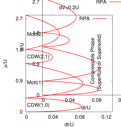
Figure 1: (Color online) We show the chemical potential $\mu$ (in units of $U$) versus hopping $t$ (in units of $U/d$) phase diagram within the random-phase approximation for $d$-dimensional hypercubic lattices (it becomes exact for $d\to\infty$). Here the nearest-neighbor repulsion scales inversely with $d$ such that $dV=0.2U$. The red solid line correspond to phase boundaries for the Mott insulator to superfluid and CDW insulator to supersolid states as obtained from Eq. (9).

When $t=0$, it turns out that the chemical potential width of all Mott and CDW lobes are $U$ and $zV$, respectively, and that the ground state alternates between the CDW and Mott phases as a function of increasing $\mu$ bruder ; parhat ; otterlo ; kuhner ; kovrizhin ; menotti ; iskin . For instance, the ground state is a vacuum $(n_{A}=0,n_{B}=0)$ for $\mu\leq 0$; it is a CDW with $(n_{A}=1,n_{B}=0)$ for $0\leq\mu\leq zV$; it is a Mott insulator with $(n_{A}=1,n_{B}=1)$ for $zV\leq\mu\leq U+zV$; it is a CDW with $(n_{A}=2,n_{B}=1)$ for $U+zV\leq\mu\leq U+2zV$; it is a Mott insulator with $(n_{A}=2,n_{B}=2)$ for $U+2zV\leq\mu\leq 2U+2zV$, and so on. As $t$ increases, the range of $\mu$ about which the ground state is insulating decreases, and the Mott and CDW phases disappear at a critical value of $t$, beyond which the system becomes compressible (superfluid or supersolid) as shown in Fig. 1.

Identification of these phases in atomic systems loaded into optical lattices is a real challenge, and the momentum distribution of particles has been the most commonly used probing technique to distinguish superfluid and Mott phases of the on-site BH model. Motivated by these experiments, next we analyze the momentum distribution of the insulating phases of the extended BH model, paying particular attention to what signatures one might see that can distinguish the CDW insulating phase.

III Momentum Distribution

The momentum distribution of the atoms is one of the few (and probably the easiest) physical quantity that can be directly probed in experiments with ultracold atomic gases. This is achieved by time-of-flight absorption imaging of freely expanding atoms that are released from the trap. Since ultracold gases are very dilute, atoms do not interact much with each other during this short time-of-flight, and therefore, the particle positions in the absorption image are strongly correlated with their velocity distribution given by their momentum distribution at the moment of release from the trap.

The momentum distribution $n(\mathbf{k})$ is also easy to calculate, and it is defined as the Fourier transform of the one-particle density matrix $\rho(\mathbf{r},\mathbf{r^{\prime}})=\langle\psi^{\dagger}(\mathbf{r})\psi(\mathbf{r^{\prime}})\rangle,$ such that

$$n(\mathbf{k})=\int d\mathbf{r}\int d\mathbf{r^{\prime}}\rho(\mathbf{r},\mathbf{r^{\prime}})e^{i\mathbf{k}\cdot(\mathbf{r}-\mathbf{r^{\prime}})},$$ (2)

where $\psi^{\dagger}(\mathbf{r})$ [$\psi(\mathbf{r})$] is the boson creation (annihilation) field operator, and $\mathbf{k}$ is the momentum. We expand the field operators in the basis set of Wannier functions such that $\psi(\mathbf{r})=(1/\sqrt{M})\sum_{\ell}W(\mathbf{r}-\mathbf{R_{\ell}})b_{\ell},$ where $M$ is the number of lattice sites, and the Wannier function $W(\mathbf{r}-\mathbf{R_{\ell}})$ is localized at site $\ell$ with position $\mathbf{R_{\ell}}$. Here the summation index $\ell\in\{A,B\}$ includes the entire lattice.

In this paper, we use two methods to calculate the momentum distribution of the insulating phases of the extended BH model. First we calculate $n(\mathbf{k})$ via the RPA theory in Sec. III.1, and its result corresponds to the exact result for the infinite-dimensional limit. Then, in Sec. III.2, we calculate $n(\mathbf{k})$ as a power series expansion in the hopping $t$ via the strong-coupling perturbation theory. We also verify that our strong-coupling expansion recovers the RPA result in the infinite-dimensional limit when the latter is expanded out in $t$ to the same order. This provides an independent cross-check of the algebra as discussed next in detail.

III.1 Random Phase Approximation (RPA)

Using the standard-basis operator method developed by Haley and Erdös haley , and following the recent works on the on-site BH model sheshadri ; sengupta ; menotti-rpa ; konabe ; ohashi , here we obtain the equation of motion for the insulating phases of the extended BH model. This approximation is a well-defined linear operation in which thermal averages of products of operators are replaced by the product of their thermal averages. In accordance with this approximation, the three-operator Green’s functions are reduced to two-operator ones haley . Therefore, the RPA method allows us to calculate the single-particle Green’s function $G(\mathbf{k},i\omega_{n})=-\langle\psi(\mathbf{k},i\omega_{n})\psi^{\dagger}(\mathbf{k},i\omega_{n})\rangle$ in momentum ($\mathbf{k}$) and Matsubara frequency ($i\omega_{n}$) space, from which the spectral function $A(\mathbf{k},\omega)=-(1/\pi){\rm Im}G(\mathbf{k},i\omega_{n}\to\omega+i\epsilon)$ can be extracted by analytical continuation. Here the angular brackets denote the standard trace over the density matrix. Notice that the spectral function should always satisfy the sum rule $\int_{-\infty}^{\infty}A(\mathbf{k},\omega)d\omega=1,$ due to the bosonic commutation relations of the creation and annihilation operators in the Heisenberg picture at equal times. Then the momentum distribution $n(\mathbf{k})=\langle\psi^{\dagger}(\mathbf{k})\psi(\mathbf{k})\rangle$ (at zero temperature) can be easily obtained from the spectral function $n(\mathbf{k})=-\int_{-\infty}^{0}A(\mathbf{k},\omega)d\omega,$ i.e.

$$n(\mathbf{k})=\frac{1}{\pi}\int_{-\infty}^{0}{\rm Im}G(\mathbf{k},i\omega_{n}\to\omega+i\epsilon)d\omega,$$ (3)

which measures the spectral weight of the hole excitation spectrum.

Expanding the field operators given in Eq. (2) in the basis set of Wannier functions, the momentum distribution becomes

$$n(\mathbf{k})=\frac{|W(\mathbf{k})|^{2}}{M}\sum_{\ell,\ell^{\prime}}\langle b_{\ell}^{\dagger}b_{\ell^{\prime}}\rangle e^{-i\mathbf{k}\cdot(\mathbf{R_{\ell}}-\mathbf{R_{\ell^{\prime}}})},$$ (4)

where $W(\mathbf{k})=\int d\mathbf{r}W(\mathbf{r})e^{i\mathbf{k}\cdot\mathbf{r}}$ is the Fourier transform of $W(\mathbf{r})$. Here the summation indices $\ell\in\{A,B\}$ and $\ell^{\prime}\in\{A,B\}$ include the entire lattice. Since $W(\mathbf{k})$ is a nonuniversal property of the lattice potential, and it has nothing to do with the extended BH model on a discrete periodic lattice, we ignore this function in this paper by setting it to unity.

But before beginning the discussion of our formal treatment of the theory, we want to comment further on the subtle features that arise for the momentum distribution $n(\mathbf{k})$ in an ordered phase, when the lattice periodicity is further broken by the spontaneous appearance of the CDW phase with a lower lattice periodicity. This system becomes that of a lattice with a basis, as the $A$ and $B$ sublattices now have a different occupancies of particles on them. When examining $n(\mathbf{k})$ on the lattice, we evaluate the one-particle density matrix at each lattice site $\rho({\bf r},{\bf r}^{\prime})\rightarrow\rho({\bf R}_{i},{\bf R}_{j})=\rho_{ij}$ (see the appendix for a further discussion of how one goes from the continuum to the lattice and how Wannier functions enter into the calculation). The integral in Eq. (2) is replaced by a summation that extends over all lattice sites of the original lattice (before the CDW order occurred). We can break this summation up into terms that involve solely the $A$ sublattice, solely the $B$ sublattice, and terms that mix the $A$ and $B$ sublattices. One can immediately see that the terms restricted to one of the sublattices are periodic with the periodicity of the reduced Brillouin zone, while the mixed terms are only periodic with respect to the full Brillouin zone. If we assume the Wannier functions are identical for the $A$ and $B$ sublattices, then this uniform weighting of the different contributions yields the correct momentum distribution; in general, one potentially has different weightings of the three different components. A full discussion of this issue is beyond this work, where we focus on the properties of the pure discrete lattice system, not on the experimental systems which have the additional real-space structure arising from the spatial continuum.

The fluctuations are not fully taken into account in the RPA method, however it goes beyond the mean-field approximation for low-dimensional systems, and it becomes exact for infinite-dimensional bosonic systems recovering the mean-field theory. The RPA method has recently been applied to describe the superfluid and Mott phases of the on-site BH model sengupta ; menotti-rpa , and its results showed good agreement with the experiments. Motivated by these earlier works, here we generalize this method to describe the insulating phases of the extended BH model.

Keeping in mind our two-sublattice system, the single-particle Green’s function in momentum and frequency space can be written as $G(\mathbf{k},i\omega_{n})=(1/2)\sum_{S,S^{\prime}}G_{SS^{\prime}}(\mathbf{k},i\omega_{n}),$ where the indices $S$ and $S^{\prime}$ label sublattices $\{A,B\}$, and $G_{SS^{\prime}}(\mathbf{k},i\omega_{n})=(2/M)\sum_{\ell\in S,\ell^{\prime}\in S^{\prime}}G_{\ell\ell^{\prime}}(i\omega_{n})e^{-i\mathbf{k}\cdot(\mathbf{R_{\ell}}-\mathbf{R_{\ell^{\prime}}})}$ is the Fourier transform. Here the summation indices $\ell\in$ $A$ or $B$ and $\ell^{\prime}\in$ $A$ or $B$ include only one sublattice and the Green’s function is defined only at the different lattice positions. Since there are $M/2$ lattice sites in one sublattice, a factor of 2 appears in this expression. Note that this is just a rewriting of the summation over all lattice sites that explicitly shows the contributions from the different sublattices. The RPA equations have the following form in position and frequency space $G_{\ell\ell^{\prime}}(i\omega_{n})=G_{\ell}^{0}(i\omega_{n})\left[\delta_{\ell\ell^{\prime}}+\sum_{\ell^{\prime\prime}}J_{\ell\ell^{\prime\prime}}G_{\ell^{\prime\prime}\ell^{\prime}}(i\omega_{n})\right],$ where $G_{\ell}^{0}(i\omega_{n})$ and $J_{\ell\ell^{\prime\prime}}$ are given below Eq. (6). Here the indices $\ell$, $\ell^{\prime}$ and $\ell^{\prime\prime}$ $\in\{A,B\}$ include the entire lattice. Using the Fourier transforms, the RPA equation in momentum and frequency space becomes $G_{SS^{\prime}}(\mathbf{k},i\omega_{n})=G_{S}^{0}(\mathbf{k},i\omega_{n})\left[\delta_{SS^{\prime}}+\sum_{S^{\prime\prime}}J_{SS^{\prime\prime}}(\mathbf{k})G_{S^{\prime\prime}S^{\prime}}(\mathbf{k},i\omega_{n})\right].$ This expression defines a set of coupled equations for the functions $G_{AA}(\mathbf{k},i\omega_{n})$, $G_{AB}(\mathbf{k},i\omega_{n})$, $G_{BA}(\mathbf{k},i\omega_{n})$ and $G_{BB}(\mathbf{k},i\omega_{n})$. These equations can be easily solved to obtain

$$G(\mathbf{k},i\omega_{n})=\frac{[G_{A}^{0}(\mathbf{k},i\omega_{n})+G_{B}^{0}(\mathbf{k},i\omega_{n})]/2+[J_{AB}(\mathbf{k})+J_{BA}(\mathbf{k})-J_{AA}(\mathbf{k})-J_{BB}(\mathbf{k})]G_{A}^{0}(\mathbf{k},i\omega_{n})G_{B}^{0}(\mathbf{k},i\omega_{n})/2}{1-J_{AA}(\mathbf{k})G_{A}^{0}(\mathbf{k},i\omega_{n})-J_{BB}(\mathbf{k})G_{B}^{0}(\mathbf{k},i\omega_{n})-[J_{AB}(\mathbf{k})J_{BA}(\mathbf{k})-J_{AA}(\mathbf{k})J_{BB}(\mathbf{k})]G_{A}^{0}(\mathbf{k},i\omega_{n})G_{B}^{0}(\mathbf{k},i\omega_{n})},$$ (5)

which corresponds to the general single-particle Green’s function within the RPA.

We use Eq. (5) to obtain the single-particle Green’s function for the insulating (Mott and CDW) phases of the extended BH model. Since hopping is allowed between nearest-neighbor sites that belong to different sublattices, in Eq. (6) we find $J_{AA}(\mathbf{k})=J_{BB}(\mathbf{k})=0$ and $J_{AB}(\mathbf{k})=J_{BA}(\mathbf{k})=\varepsilon(\mathbf{k})$, where $\varepsilon(\mathbf{k})$ is the Fourier transform of the hopping matrix (also called the band structure). For $d$-dimensional hypercubic lattices considered in this paper, the energy dispersion becomes $\varepsilon(\mathbf{k})=-2t\sum_{i=1}^{d}\cos(k_{i}a),$ where $a$ is the lattice spacing. This then yields the following expression for the Green’s function:

$$G_{\rm Ins}(\mathbf{k},i\omega_{n})=\frac{G_{\rm avr}^{0}(i\omega_{n})+\varepsilon(\mathbf{k})G_{A}^{0}(i\omega_{n})G_{B}^{0}(i\omega_{n})}{1-\varepsilon^{2}(\mathbf{k})G_{A}^{0}(i\omega_{n})G_{B}^{0}(i\omega_{n})},$$ (6)

where $G_{\rm avr}^{0}(i\omega_{n})=\left[G_{A}^{0}(i\omega_{n})+G_{B}^{0}(i\omega_{n})\right]/2$. The $\mathbf{k}$-independent functions $G_{A}^{0}(i\omega_{n})$ and $G_{B}^{0}(i\omega_{n})$ correspond to the single-particle local Green’s functions for sublattices $A$ and $B$, respectively, at zeroth order in $t$. They have the familiar form

$$G_{A}^{0}(i\omega_{n}) =\frac{n_{A}+1}{i\omega_{n}-E_{A}^{\rm par}}-\frac{n_{A}}{i\omega_{n}+E_{A}^{\rm hol}},$$ (7)

$$G_{B}^{0}(i\omega_{n}) =\frac{n_{B}+1}{i\omega_{n}-E_{B}^{\rm par}}-\frac{n_{B}}{i\omega_{n}+E_{B}^{\rm hol}},$$ (8)

where $E_{A}^{\rm par}=Un_{A}+zVn_{B}-\mu$ and $E_{B}^{\rm par}=Un_{B}+zVn_{A}-\mu$ are the zeroth-order particle excitation spectrum in $t$ (the energy required to add one extra particle) for sublattices $A$ and $B$, respectively, and similarly $E_{A}^{\rm hol}=-U(n_{A}-1)-zVn_{B}+\mu$ and $E_{B}^{\rm hol}=-U(n_{B}-1)-zVn_{A}+\mu$ are the zeroth-order hole excitation spectrum in $t$ (the energy required to remove one particle). Notice that $G_{\rm Ins}(\mathbf{k},i\omega_{n})=G_{\rm avr}^{0}(i\omega_{n})$ at zeroth order in $t$, as one may expect.

The poles of $G_{\rm Ins}(\mathbf{k},i\omega_{n})$, i.e. the condition $1=\varepsilon^{2}(\mathbf{k})G_{A}^{0}(i\omega_{n})G_{B}^{0}(i\omega_{n})$, give the $\mathbf{k}$-dependence of the particle and hole excitation spectrum. The insulating phase becomes unstable against superfluidity when any of the excitation energies becomes negative at $\mathbf{k}=0$. In addition, the poles of $G_{\rm Ins}(\mathbf{k},i\omega_{n})$ at $(\mathbf{k}=\mathbf{0},i\omega_{n}=0)$, i.e. the condition $1=\varepsilon^{2}(\mathbf{0})G_{A}^{0}(0)G_{B}^{0}(0)$, gives the mean-field phase boundary between the incompressible (Mott or CDW) and the compressible (superfluid or supersolid) phases. This condition leads to

$$\frac{1}{z^{2}t^{2}} =\left(\frac{n_{A}+1}{E_{A}^{\rm par}}+\frac{n_{A}}{E_{A}^{\rm hol}}\right)\left(\frac{n_{B}+1}{E_{B}^{\rm par}}+\frac{n_{B}}{E_{B}^{\rm hol}}\right),$$ (9)

which is a quartic equation for $\mu$, and it coincides with our earlier result iskin . Notice that Eq. (9) reduces to the usual expression for the phase boundary of the on-site BH model when $n_{A}=n_{B}=n_{0}$ and $V=0$. Having discussed the general RPA formalism for the insulating phases of the extended BH model, next we analyze the momentum distribution of the Mott and CDW phases separately.

III.1.1 Mott Phase

The single-particle Green’s function for the Mott phase can be obtained from Eq. (6) by setting $n_{A}=n_{B}=n_{0}$. This leads to

$$G_{\rm Mott}(\mathbf{k},i\omega_{n})=\frac{G_{0}^{0}(i\omega_{n})}{1-\varepsilon(\mathbf{k})G_{0}^{0}(i\omega_{n})},$$ (10)

which has the same form with that of the Green’s function of the Mott phase in the on-site BH model sengupta ; ohashi ; menotti-rpa . Here, $G_{A}^{0}(i\omega_{n})=G_{B}^{0}(i\omega_{n})=G_{0}^{0}(i\omega_{n})$. The function $G_{\rm Mott}(\mathbf{k},i\omega_{n})$ has two poles at $i\omega_{n}=E_{0}^{\rm par}(\mathbf{k})$ and $i\omega_{n}=-E_{0}^{\rm hol}(\mathbf{k})$,

$$E_{0}^{\rm par}(\mathbf{k}) =E_{0}^{\rm par}-\left[U-\varepsilon(\mathbf{k})-E_{0}(\mathbf{k})\right]/2,$$ (11)

$$E_{0}^{\rm hol}(\mathbf{k}) =E_{0}^{\rm hol}-\left[U+\varepsilon(\mathbf{k})-E_{0}(\mathbf{k})\right]/2,$$ (12)

corresponding to the particle (the energy required to add one extra particle) and hole (the energy required to remove one particle) excitation spectrum, respectively, where $E_{0}(\mathbf{k})=\sqrt{\varepsilon^{2}(\mathbf{k})+2U(2n_{0}+1)\varepsilon(\mathbf{k})+U^{2}}.$ Notice that the Mott insulator becomes unstable against superfluidity when $E_{0}^{\rm par}(\mathbf{0})=0$ or $E_{0}^{\rm hol}(\mathbf{0})=0$, and these conditions coincide with the mean-field condition given in Eq. (9) when $n_{A}=n_{B}=n_{0}$.

Therefore, the Green’s function for the Mott phase can be written as

$$G_{\rm Mott}(\mathbf{k},i\omega_{n})=\frac{C_{0}^{\rm par}(\mathbf{k})}{i\omega_{n}-E_{0}^{\rm par}(\mathbf{k})}+\frac{C_{0}^{\rm hol}(\mathbf{k})}{i\omega_{n}+E_{0}^{\rm hol}(\mathbf{k})},$$ (13)

where the coefficients (or the spectral weights) are functions of the excitation spectrum

$$C_{0}^{\rm par}(\mathbf{k}) =\frac{E_{0}^{\rm par}(\mathbf{k})+Un_{0}+E_{0}^{\rm hol}}{E_{0}^{\rm par}(\mathbf{k})+E_{0}^{\rm hol}(\mathbf{k})},$$ (14)

$$C_{0}^{\rm hol}(\mathbf{k}) =\frac{E_{0}^{\rm hol}(\mathbf{k})-Un_{0}-E_{0}^{\rm hol}}{E_{0}^{\rm par}(\mathbf{k})+E_{0}^{\rm hol}(\mathbf{k})}.$$ (15)

Using the definition given above Eq. (3), the spectral function for the Mott phase can be easily obtained from Eq. (13), leading to $A_{\rm Mott}(\mathbf{k},\omega)=C_{0}^{\rm par}(\mathbf{k})\delta[\omega-E_{0}^{\rm par}(\mathbf{k})]+C_{0}^{\rm hol}(\mathbf{k})\delta[\omega+E_{0}^{\rm hol}(\mathbf{k})],$ where $\delta(x)$ is the Delta function defined by $\delta(x)=(1/\pi)\lim_{\epsilon\to 0}\epsilon/(x^{2}+\epsilon^{2}).$ Notice that this function satisfies the sum rule mentioned above Eq. (3), since the coefficients satisfy $C_{0}^{\rm par}(\mathbf{k})+C_{0}^{\rm par}(\mathbf{k})=1$. The momentum distribution measures the spectral weight of the hole excitation spectrum as defined in Eq. (3), and for the Mott phase it is given by

$$n_{\rm Mott}(\mathbf{k})=-C_{0}^{\rm hol}(\mathbf{k})=\frac{U(2n_{0}+1)+\varepsilon(\mathbf{k})}{2E_{0}(\mathbf{k})}-\frac{1}{2},$$ (16)

which is identical to the $n_{\rm Mott}(\mathbf{k})$ of the on-site BH model sengupta ; menotti-rpa . Therefore, at the RPA level, $n_{\rm Mott}(\mathbf{k})$ is independent of $V$ which is mainly because of the underlying mean-field Hamiltonian that is used in the RPA formalism (we remind that fluctuations are not fully taken into account within RPA). For instance, the mean-field phase boundary condition given in Eq. (9) shows that the Mott lobes are separated by $zV$, but their shapes and, in particular, the critical points are independent of $V$. This point will become more clear in Sec. III.2, where we analyze $n(\mathbf{k})$ via the strong-coupling perturbation theory up to second order in $t$. Notice that the momentum distribution is flat and equals the average filling fraction $n_{\rm Mott}(\mathbf{k})=n_{0}$ at zeroth order in $t$, corresponding to vanishing site-to-site correlations.

III.1.2 CDW Phase

In contrast to the Green’s function of the Mott phase, the single-particle Green’s function for the CDW phase $G_{\rm CDW}(\mathbf{k},i\omega_{n})$ has four poles. Two of them correspond to the particle and the other two to the hole excitation spectrum of sublattices $A$ and $B$. Unfortunately, general expressions for these poles are not analytically tractable since the condition $1=\varepsilon^{2}(\mathbf{k})G_{A}^{0}(i\omega_{n})G_{B}^{0}(i\omega_{n})$ defines a quartic equation for $i\omega_{n}$; they can be easily obtained numerically for any given CDW lobe as shown in Sec. III.3. Assuming that the excitation spectrum is known, the Green’s function for the CDW phase can be written as

$$G_{\rm CDW} (\mathbf{k},i\omega_{n})=\frac{C_{A}^{\rm par}(\mathbf{k})}{i\omega_{n}-E_{A}^{\rm par}(\mathbf{k})}+\frac{C_{A}^{\rm hol}(\mathbf{k})}{i\omega_{n}+E_{A}^{\rm hol}(\mathbf{k})}$$

$$+\frac{C_{B}^{\rm par}(\mathbf{k})}{i\omega_{n}-E_{B}^{\rm par}(\mathbf{k})}+\frac{C_{B}^{\rm hol}(\mathbf{k})}{i\omega_{n}+E_{B}^{\rm hol}(\mathbf{k})},$$ (17)

where $E_{A}^{\rm par}(\mathbf{k})$ and $E_{B}^{\rm par}(\mathbf{k})$ are the particle (the energy required to add one extra particle) and $E_{A}^{\rm hol}(\mathbf{k})$ and $E_{B}^{\rm hol}(\mathbf{k})$ are the hole (the energy required to remove one particle) excitation spectrum. The coefficients (or the spectral weights) are functions of the excitation spectrum, such that

$$C_{A}^{\rm par}(\mathbf{k})=\frac{D_{0}(\mathbf{k})+D_{1}(\mathbf{k})E_{A}^{\rm par}(\mathbf{k})+D_{2}(\mathbf{k})[E_{A}^{\rm par}(\mathbf{k})]^{2}+[E_{A}^{\rm par}(\mathbf{k})]^{3}}{[E_{A}^{\rm par}(\mathbf{k})-E_{B}^{\rm par}(\mathbf{k})][E_{A}^{\rm par}(\mathbf{k})+E_{B}^{\rm hol}(\mathbf{k})][E_{A}^{\rm par}(\mathbf{k})+E_{A}^{\rm hol}(\mathbf{k})]},$$ (18)

$$C_{B}^{\rm par}(\mathbf{k})=\frac{D_{0}(\mathbf{k})+D_{1}(\mathbf{k})E_{B}^{\rm par}(\mathbf{k})+D_{2}(\mathbf{k})[E_{B}^{\rm par}(\mathbf{k})]^{2}+[E_{B}^{\rm par}(\mathbf{k})]^{3}}{[E_{B}^{\rm par}(\mathbf{k})-E_{A}^{\rm par}(\mathbf{k})][E_{B}^{\rm par}(\mathbf{k})+E_{A}^{\rm hol}(\mathbf{k})][E_{B}^{\rm par}(\mathbf{k})+E_{B}^{\rm hol}(\mathbf{k})]},$$ (19)

$$C_{A}^{\rm hol}(\mathbf{k})=\frac{D_{0}(\mathbf{k})-D_{1}(\mathbf{k})E_{A}^{\rm hol}(\mathbf{k})+D_{2}(\mathbf{k})[E_{A}^{\rm hol}(\mathbf{k})]^{2}-[E_{A}^{\rm hol}(\mathbf{k})]^{3}}{[E_{B}^{\rm hol}(\mathbf{k})-E_{A}^{\rm hol}(\mathbf{k})][E_{A}^{\rm hol}(\mathbf{k})+E_{B}^{\rm par}(\mathbf{k})][E_{A}^{\rm hol}(\mathbf{k})+E_{A}^{\rm par}(\mathbf{k})]},$$ (20)

$$C_{B}^{\rm hol}(\mathbf{k})=\frac{D_{0}(\mathbf{k})-D_{1}(\mathbf{k})E_{B}^{\rm hol}(\mathbf{k})+D_{2}(\mathbf{k})[E_{B}^{\rm hol}(\mathbf{k})]^{2}-[E_{B}^{\rm hol}(\mathbf{k})]^{3}}{[E_{A}^{\rm hol}(\mathbf{k})-E_{B}^{\rm hol}(\mathbf{k})][E_{B}^{\rm hol}(\mathbf{k})+E_{B}^{\rm par}(\mathbf{k})][E_{B}^{\rm hol}(\mathbf{k})+E_{A}^{\rm par}(\mathbf{k})]}.$$ (21)

Here, the coefficients $D_{0}(\mathbf{k})$, $D_{1}(\mathbf{k})$, and $D_{2}(\mathbf{k})$ are functions of the zeroth-order excitation spectrum in $t$ defined below Eq. (8), and are given by

$$D_{0} (\mathbf{k})=-\left[E_{A}^{\rm par}E_{A}^{\rm hol}(Un_{B}+E_{B}^{\rm hol})+E_{B}^{\rm par}E_{B}^{\rm hol}\right.$$

$$\left.(Un_{A}+E_{A}^{\rm hol})\right]/2+\varepsilon(\mathbf{k})(Un_{A}+E_{A}^{\rm hol})(Un_{B}+E_{B}^{\rm hol}),$$ (22)

$$D_{1} (\mathbf{k})=\left[(E_{A}^{\rm hol}-E_{A}^{\rm par})(Un_{B}+E_{B}^{\rm hol})+(E_{B}^{\rm hol}-E_{B}^{\rm par})\right.$$

$$\left.(Un_{A}+E_{A}^{\rm hol})-E_{A}^{\rm par}E_{A}^{\rm hol}-E_{B}^{\rm par}E_{B}^{\rm hol}\right]/2$$

$$+\varepsilon(\mathbf{k})(Un_{A}+Un_{B}+E_{A}^{\rm hol}+E_{B}^{\rm hol}),$$ (23)

and

$$D_{2} (\mathbf{k})=\left(Un_{A}+Un_{B}-E_{A}^{\rm par}-E_{B}^{\rm par}\right)/2+E_{A}^{\rm hol}+E_{B}^{\rm hol}$$

$$+\varepsilon(\mathbf{k}).$$ (24)

Using the definition given above Eq. (3), the spectral function for the CDW phase can be easily obtained from Eq. (III.1.2), leading to $A_{\rm CDW}(\mathbf{k},\omega)=C_{A}^{\rm par}(\mathbf{k})\delta[\omega-E_{A}^{\rm par}(\mathbf{k})]+C_{A}^{\rm hol}(\mathbf{k})\delta[\omega+E_{A}^{\rm hol}(\mathbf{k})]+C_{B}^{\rm par}(\mathbf{k})\delta[\omega-E_{B}^{\rm par}(\mathbf{k})]+C_{B}^{\rm hol}(\mathbf{k})\delta[\omega+E_{B}^{\rm hol}(\mathbf{k})].$ Notice that this function satisfies the sum rule mentioned above Eq. (3), since the coefficients satisfy $C_{A}^{\rm par}(\mathbf{k})+C_{A}^{\rm hol}(\mathbf{k})+C_{B}^{\rm par}(\mathbf{k})+C_{B}^{\rm hol}(\mathbf{k})=1.$ The momentum distribution measures the spectral weight of the hole excitation spectrum as defined in Eq. (3), and for the CDW phase it is given by

$$n_{\rm CDW}(\mathbf{k})=-C_{A}^{\rm hol}(\mathbf{k})-C_{B}^{\rm hol}(\mathbf{k}).$$ (25)

This expression has a highly non-trivial dependence on $t$, and it has to be solved numerically together with the excitation spectrum. However, it can be analytically shown that the momentum distribution is flat and equals the average filling fraction $n_{\rm CDW}(\mathbf{k})=(n_{A}+n_{B})/2$ at zeroth order in $t$, corresponding to vanishing site-to-site correlations. To provide an independent check of the algebra (and to extend to finite dimensions), we next calculate $n(\mathbf{k})$ as a power series expansion in the hopping $t$ via the exact strong-coupling perturbation theory in $d$ dimensions.

III.2 Strong-coupling Perturbation Theory

To determine the momentum distribution of the insulating phases, we need the wavefunction of the insulating state $|\Psi_{\rm Ins}\rangle$ as a function of $t$. We use the many-body version of Rayleigh-Schrödinger perturbation theory in the kinetic energy term landau to perform the expansion (in powers of $t$) for $|\Psi_{\rm Ins}\rangle$ needed to carry out our analysis. A similar expansion for the ground-state energies was previously used to discuss the phase diagram of the on-site BH model freericks-1 ; freericks-2 , and it has recently been applied to the extended BH model iskin . For the on-site BH model, extrapolated results of these expansions showed an excellent agreement with recent quantum Monte Carlo simulations prokofiev-1 ; prokofiev-2 . A high-order strong-coupling expansion for the ground-state energies has now been extended to all dimensions and fillings holthaus , and a high-order expansion for the wavefunction has also been used to describe the Mott phase in one-dimensional systems damski .

For our purpose, we first need the ground-state wavefuntions of the Mott and CDW phases when $t=0$. To zeroth order in $t$, the insulator (Mott or CDW) wavefunction can be written as

$$|\Psi_{\rm Ins}^{(0)}\rangle = \prod_{\ell\in A,\ell^{\prime}\in B}^{M/2}\frac{(b_{\ell}^{\dagger})^{n_{A}}}{\sqrt{n_{A}!}}\frac{(b_{\ell^{\prime}}^{\dagger})^{n_{B}}}{\sqrt{n_{B}!}}|0\rangle,$$ (26)

where $M$ is the number of lattice sites, and $|0\rangle$ is the vacuum state (here, we remind that the lattice is divided equally into $A$ and $B$ sublattices). In principle, we can apply the perturbation theory on $|\Psi_{\rm Ins}^{(0)}\rangle$ to calculate $|\Psi_{\rm Ins}\rangle$ up to the desired order. However, since the number of intermediate states increases dramatically due to the presence of nearest-neighbor interactions, we perform this expansion only up to second order in $t$. The (unnormalized) wavefunction for the insulating state can then be written as

$$|\psi_{\rm Ins}\rangle =|\Psi_{\rm Ins}^{(0)}\rangle+\sum_{m\neq|\Psi_{\rm Ins}^{(0)}\rangle}\frac{T_{m0}}{E_{0m}}|\Psi_{\rm Ins}^{(0)}\rangle$$

$$+\sum_{\{m^{\prime},m\}\neq|\Psi_{\rm Ins}^{(0)}\rangle}\frac{T_{m^{\prime}m}T_{m0}}{E_{0m^{\prime}}E_{0m}}|\Psi_{\rm Ins}^{(0)}\rangle+O(t^{3}),$$ (27)

where $T_{m0}=-\sum_{S,S^{\prime}}\sum_{\ell\in S,\ell^{\prime}\in S^{\prime}}t_{\ell\ell^{\prime}}\langle m|b_{\ell}^{\dagger}b_{\ell^{\prime}}|\Psi_{\rm Ins}^{(0)}\rangle$ is the hopping matrix element between the first-order intermediate state $|m\rangle$ and the zeroth-order state $|\Psi_{\rm Ins}^{(0)}\rangle$, and $T_{mm^{\prime}}$ is between $|m\rangle$ and the second-order intermediate state $|m^{\prime}\rangle$, and $E_{0m}=E_{\rm Ins}^{(0)}-E_{m}^{(0)}$. Here the summation indices $\ell\in\{A,B\}$ and $\ell^{\prime}\in\{A,B\}$ include the entire lattice, and $S$ and $S^{\prime}$ label sublattices $\{A,B\}$. The $|m\rangle$ states are connected to $|\Psi_{\rm Ins}^{(0)}\rangle$ state with a single hopping, and similarly $|m^{\prime}\rangle$ states are connected to $|m\rangle$ states with a single hopping. However, the $|m^{\prime}\rangle$ state must be different from the $|\Psi_{\rm Ins}^{(0)}\rangle$ state.

To calculate the momentum distribution, we need the normalized wavefunction for the insulating state $|\Psi_{\rm Ins}\rangle=|\psi_{\rm Ins}\rangle/\sqrt{\langle\psi_{\rm Ins}|\psi_{\rm Ins}\rangle},$ where the normalization up to second order in $t$ is given by

$$\langle \psi_{\rm Ins}|\psi_{\rm Ins}\rangle=1+\frac{n_{A}(n_{B}+1)Mzt^{2}/2}{\left[U(n_{A}-n_{B}-1)+V(zn_{B}-zn_{A}+1)\right]^{2}}$$

$$+\frac{n_{B}(n_{A}+1)Mzt^{2}/2}{\left[U(n_{B}-n_{A}-1)+V(zn_{A}-zn_{B}+1)\right]^{2}}+O(t^{4}).$$ (28)

Here, $z=2d$ is the lattice coordination number. Since $\langle m|\Psi_{\rm Ins}^{(0)}\rangle=\langle m^{\prime\prime}|\Psi_{\rm Ins}^{(0)}\rangle=\langle m^{\prime}|m\rangle=0$, the first and third order terms in $t$ vanish in the normalization. In general, all odd-order terms in $t$ vanish.

A lengthy but straightforward calculation leads to the momentum distribution, [defined in Eq. (4)] $n(\mathbf{k})=(1/M)\sum_{\ell,\ell^{\prime}}\langle\Psi_{\rm Ins}|b_{\ell}^{\dagger}b_{\ell^{\prime}}|\Psi_{\rm Ins}\rangle e^{-i\mathbf{k}\cdot(\mathbf{R_{\ell}}-\mathbf{R_{\ell^{\prime}}})},$ up to second order in $t$ as

$$n_{\rm Ins}(\mathbf{k}) =\frac{n_{A}+n_{B}}{2}+\left[\frac{n_{A}(n_{B}+1)}{U(n_{A}-n_{B}-1)+V(zn_{B}-zn_{A}+1)}+\frac{n_{B}(n_{A}+1)}{U(n_{B}-n_{A}-1)+V(zn_{A}-zn_{B}+1)}\right]\varepsilon(\mathbf{k})$$

$$+\Big{\{}\frac{n_{A}(n_{B}+1)}{2\left[U(n_{A}-n_{B}-1)+V(zn_{B}-zn_{A}+1)\right]^{2}}+\frac{n_{B}(n_{A}+1)}{2\left[U(n_{B}-n_{A}-1)+V(zn_{A}-zn_{B}+1)\right]^{2}}$$

$$-\frac{n_{A}(n_{B}+1)}{U\left[U(n_{A}-n_{B}-1)+V(zn_{B}-zn_{A}+1)\right]}-\frac{n_{B}(n_{A}+1)}{U\left[U(n_{B}-n_{A}-1)+V(zn_{A}-zn_{B}+1)\right]}\Big{\}}$$

$$(n_{A}+n_{B}+1)\left[\varepsilon^{2}(\mathbf{k})-2dt^{2}\right]+O(t^{3}).$$ (29)

In the definition of the momentum distribution, the summation indices $\ell\in\{A,B\}$ and $\ell^{\prime}\in\{A,B\}$ include the entire lattice. Here $\varepsilon(\mathbf{k})=-(2/M)\sum_{\ell\in S,\ell^{\prime}\in S^{\prime}}t_{\ell\ell^{\prime}}e^{i\mathbf{k}\cdot(\mathbf{R_{\ell}}-\mathbf{R_{\ell^{\prime}}})}$ is the Fourier transform of the hopping matrix $t_{\ell,\ell^{\prime}}$ (energy dispersion), and $\varepsilon^{2}(\mathbf{k})-2dt^{2}=(2/M)\sum_{\{\ell,\ell^{\prime\prime}\}\in S,\ell^{\prime}\in S^{\prime}}t_{\ell\ell^{\prime}}t_{\ell^{\prime}\ell^{\prime\prime}}e^{i\mathbf{k}\cdot(\mathbf{R_{\ell}}-\mathbf{R_{\ell^{\prime\prime}}})},$ where the summation indices $\{\ell,\ell^{\prime\prime}\}\in$ $A$ (or $B$) and $\ell^{\prime}\in$ $B$ (or $A$) include only one sublattice. Since there are $M/2$ lattice sites in one sublattice, a factor of 2 appears in these expressions. To zeroth order in $t$, Eq. (III.2) shows that $n_{\rm Ins}(\mathbf{k})$ is flat and equals the average filling fraction $(n_{A}+n_{B})/2$. However, it develops a peak around $\mathbf{k}=\mathbf{0}$ and a minimum around $\mathbf{k}=\mathbf{\pi}$ at first order in $t$. These general observations are consistent with the RPA results shown in Eqs. (16) and (25).

Equation (III.2) is valid for the insulating phases of all $d$-dimensional hypercubic lattices. For instance, when $n_{A}=n_{B}=n_{0}$, Eq. (III.2) reduces to the momentum distribution for the Mott phase, i.e.

$$n_{\rm Mott} (\mathbf{k})=n_{0}-2n_{0}(n_{0}+1)\frac{\varepsilon(\mathbf{k})}{U-V}+n_{0}(n_{0}+1)$$

$$(2n_{0}+1)\left[\varepsilon^{2}(\mathbf{k})-2dt^{2}\right]\frac{3U-2V}{U(U-V)^{2}}+O(t^{3}).$$ (30)

This expression recovers the known result for the on-site BH model when $V=0$ freericks-3 ; hoffmann . In addition, in the $d\to\infty$ limit, we checked that Eqs. (III.2) and (III.2) agree with the RPA solutions (which are exact in this limit) given in Eqs. (25) and (16) when the latter are expanded out to second order in $t$, providing an independent check of the algebra. One must note that the terms $2V$ and $V$ that appear in the numerator and denominator of Eq. (III.2) vanish in the limit when $d\to\infty$ because $V\propto 1/d$. Next we compare the RPA results with those of the strong-coupling perturbation theory.

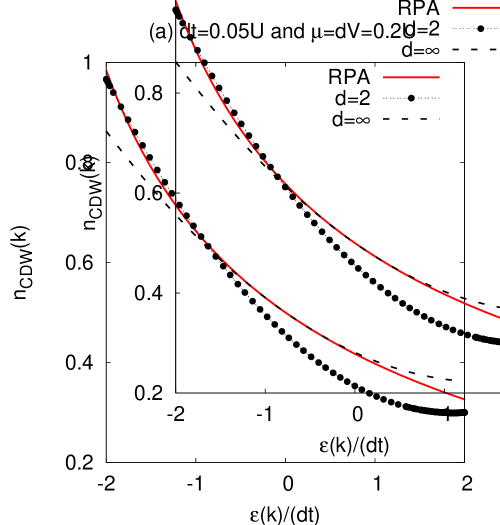
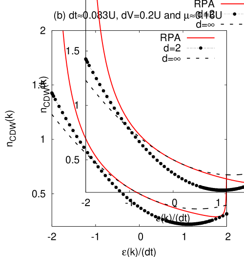
Figure 2: (Color online) Momentum distribution $n_{\rm CDW}(\mathbf{k})$ versus $\varepsilon(\mathbf{k})/(dt)$ for a $(d=2)$- and $(d\to\infty)$-dimensional hypercubic lattices. Panel (a) has the nearest-neighbor boson-repulsion satisfying $dV=0.2U$, the hopping satisfying $dt=0.05U$ and the chemical potential set by $\mu=0.2U$ corresponding approximately to the center of the first CDW lobe, and panel (b) has $dV=0.2U$, $dt\approx 0.083U$, and $\mu\approx 0.16$ corresponding approximately to the tip of the first CDW lobe. The solid (red) lines correspond to the RPA, and the dashed and circled lines to the second-order strong-coupling perturbation theory for different dimensions. The peak occurs at the zone corner only when the hopping is close to the tip of the CDW lobe.

III.3 Numerical Results

Since the momentum distribution of the CDW phase given in Eq. (25) has a highly nontrivial dependence on $t$, it has to be solved numerically together with the excitation spectrum. Next we set $dV=0.2U$ and solve this equation for the first CDW lobe. For this parameter, we remind that the $t=0$ chemical potential width of all Mott and CDW lobes are $U$ and $0.4U$, respectively, and that the ground state alternates between the CDW and Mott phases as a function of $\mu$. For instance, the ground state is a vacuum $(n_{0}=0)$ for $\mu\leq 0$; it is a CDW with $(n_{A}=1,n_{B}=0)$ for $0\leq\mu\leq 0.4U$; it is a Mott insulator with $(n_{0}=1)$ for $0.4U\leq\mu\leq 1.4U$; it is a CDW with $(n_{A}=2,n_{B}=1)$ for $1.4U\leq\mu\leq 1.8U$; it is a Mott insulator with $(n_{0}=2)$ for $1.8U\leq\mu\leq 2.8U$.

In Fig. 2, the results of the RPA calculation given in Eq. (25) are compared to those of the second-order strong-coupling perturbation theory given in Eq. (III.2) for a $(d=2)$- and $(d\to\infty)$-dimensional hypercubic lattices. In this figure, we show the momentum distribution $n_{\rm CDW}(\mathbf{k})$ as a function of $\varepsilon(\mathbf{k})/(dt)$ for two sets of parameters. In Fig. 2(a), we choose $dt=0.05U$ and $\mu=0.2U$ which approximately corresponds to the center of the first CDW lobe. For this parameter set, deep inside the CDW lobe, the momentum distribution has a peak at $\varepsilon(\mathbf{k})=-2dt$ corresponding to the $\mathbf{k}=\mathbf{0}$ point, and it has a minimum at $\varepsilon(\mathbf{k})=2dt$ corresponding to the $\mathbf{k}=(\pi,\pi,\ldots)$ point. This is very similar to what happens in the Mott phase. However, in Fig. 2(b), we choose $dt\approx 0.083U$ and $\mu\approx 0.16U$ which approximately corresponds to the tip of the first CDW lobe. For this parameter set, close to the CDW-supersolid phase transition, the momentum distribution has two peaks: a large peak at $\varepsilon(\mathbf{k})=-2dt$ corresponding to the $\mathbf{k}=\mathbf{0}$ point, and a smaller one at $\varepsilon(\mathbf{k})=2dt$ corresponding to the $\mathbf{k}=(\pi,\pi,\ldots)$ point. The second peak is unique to the CDW phase and it does not occur in a Mott phase. Notice that both the RPA and second-order strong-coupling expansion give qualitatively similar results (although the peak is much sharper and has lower weight in the exact solution).

One might have expected to always see the peak in the momentum distribution at the $\mathbf{k}=(\pi,\pi,\ldots)$ point due to the reduced periodicity of the CDW order. But because the momentum distribution involves four terms corresponding the the $AA$, $AB$, $BA$, and $BB$ sublattice combinations, only the first and last terms are periodic in the reduced Brillouin zone (see our discussion given in the appendix). Deep inside the CDW lobe, the presence of a large gap in the one-particle excitation spectrum produces an exponential decay of the one-particle correlations which suppresses this peak in the momentum distribution as can be seen in Fig. 2(a) (this point has already been discussed in Ref. rigol, ). This essentially occurs because there is a cancellation of the peak that arises from the $AA$ and $BB$ contributions with the results from the $AB$ and $BA$ pieces, similar to what happens in the Mott phase. However, close to the tip of the CDW lobe, the peak emerges in the exact solution of the RPA as shown in Fig. 2(b). To some extent, this peak also emerges in the solutions of the second-order strong-coupling perturbation theory. Notice that the peak is underemphasized in the strong-coupling theory since the theory is exact only deep inside the CDW lobe, and it becomes quantitatively inaccurate for large values of $dt/U$ close to the tip of the CDW lobe. We remark that an unphysical peak appears at $\mathbf{k}=(\pi,\pi,\ldots)$ in the strong-coupling perturbation theory for the Mott phase (not shown), which signals the breakdown of the second-order expansion.

As a further check of the accuracy of our second-order strong-coupling expansion, in Fig. 3 we compare the $d=2$ and $d\to\infty$ limits of Eq. (III.2) to the RPA method given in Eq. (25) which corresponds to the exact solution in the latter limit. In this figure, we show $n_{\rm CDW}(\mathbf{k}=\mathbf{0})$ and $n_{\rm CDW}(\mathbf{k}=\mathbf{\pi})$ as a function of $dt/U$ when $\mu=0.2U$. In $d=2$ dimensions, the RPA and second-order strong-coupling expansion gives qualitatively similar results for small values of $dt/U$, i.e. deep inside the CDW lobe. However, in the $d\to\infty$ limit, the results of the RPA and the second-order strong-coupling expansion match exactly for small values of $dt/U$ (as they must). Close to the tip of the CDW lobe, the RPA and strong-coupling results differ substantially from each other signalling the breakdown of the second-order expansion. However, both theories show that $n_{\rm CDW}(\mathbf{0})$ is an increasing function of $dt/U$ as one may expect. This is because the range of $\mu$ about which the ground state is a CDW decreases as $dt/U$ increases from zero, and the CDW phase become a supersolid at a critical value of $dt_{c}\sim 0.08U$. Beyond this point, $n(\mathbf{0})$ diverges due to the appearance of a condensate, corresponding to the macroscopic occupation of the $\mathbf{k}=\mathbf{0}$ state.

Note that we do not attempt to perform a scaling analysis of the momentum distribution for the CDW phase. The reasons why are twofold. First, we only have the series through second order, which probably is too short to be able to properly fit to a phenomenological scaling form, and second, we cannot extract the analytic scaling form from the RPA calculation anymore, so guessing an appropriate phenomenological form has less guidance than for the Mott phase. A scaled theory would be expected to be accurate for all values of $t$ within the insulating phases, as has been recently shown for the Mott phase of the on-site BH model freericks-3 .

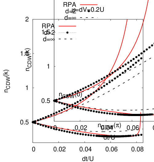
Figure 3: (Color online) Momentum ditributions at specific momentum points $n_{\rm CDW}(\mathbf{k}=\mathbf{0})$ and $n_{\rm CDW}(\mathbf{k}=\mathbf{\pi})$ versus $dt/U$ for $(d=2)$- and $(d\to\infty)$-dimensional hypercubic lattices. The chemical potential $\mu=dV$ corresponds to the first CDW lobe, and the nearest-neighbor repulsion is set to $dV=0.2U$. The solid line corresponds to the RPA and the dashed and circled lines to the second-order strong-coupling perturbation theory for different dimensions.

IV Conclusions

We developed two methods to calculate the momentum distribution of the insulating (Mott and charge-density-wave) phases of the extended Bose-Hubbard model with on-site and nearest-neighbor boson-boson repulsions on $d$-dimensional hypercubic lattices. First we analyzed the momentum distribution within the random phase approximation, which corresponds to the exact solution for the infinite-dimensional limit. Then we used the many-body version of the Rayleigh-Schrödinger perturbation theory in the kinetic-energy term, and derived the wavefunction for the insulating phases as a power series in the hopping $t$, to calculate the momentum distribution via the strong-coupling perturbation theory. A similar strong-coupling expansion for the ground-state energies was previously used to discuss the phase diagram of the on-site BH model freericks-1 ; freericks-2 , and it has recently been applied to the extended BH model iskin .

The agreement between the second-order strong-coupling expansion and that of RPA method is only qualitative in low-dimensional systems. This is not surprising since the fluctuations are not fully taken into account in the RPA method. However, we showed that our strong-coupling expansion matches exactly the RPA result (as it must) in the infinite-dimensional limit when the latter is expanded out in $t$ to the same order. We believe some of these results could potentially be tested with ultracold dipolar Bose gases loaded into optical lattices. This work can be extended in several ways if desired. For instance, one could calculate the momentum distribution up to third order in $t$, and develop a scaling theory with the help of the RPA results (or a good phenomenological guess for the scaling form of the momentum distribution). The scaled theory is expected to be accurate for all values of $t$ within the insulating phases, as has been recently shown for the Mott phase of the on-site BH model freericks-3 .

V Acknowledgements

We would like to acknowledge useful discussions with H. R. Krishnamurthy and M. Rigol. J. K. F. acknowledges support under the USARO Grant W911NF0710576 with funds from the DARPA OLE Program.

Appendix A Effective CDW Hamiltonian

In this Appendix, we comment on some of the subtle issues regarding Wannier functions in the CDW phase. When the particle occupancies show a CDW order, we can think of the combination of the CDW order plus the lattice potential as an effective lattice potential such that the effective potential is different for each sublattice. In other words, CDW order creates an effective potential which depends on the particle occupation of the sublattice. In fact, having different effective lattice potentials on two sublattices could be thought of as the reason for having a CDW order at the first place. Equivalently, this is like considering the mean-field Hamiltonian with CDW order as the starting point for determining the Wannier wavefunctions, with the symmetry explicitly broken between the $A$ and $B$ sublattices.

This observation suggests that in contrast to the Mott phase where all lattice sites are identical and the Wannier functions are exactly the same for both sublattices, i.e. $W_{A}(\mathbf{r})=W_{B}(\mathbf{r})=W_{0}(\mathbf{r})$, the Wannier functions depend on the sublattice when the CDW order exists, i.e. $W_{A}(\mathbf{r})\neq W_{B}(\mathbf{r})$. Throughout this paper, we assume that the Wannier functions are equal (or at least similar) in sublattices $A$ and $B$. However, depending on the CDW order (e.g. $n_{A}\gg n_{B}$) and the lattice potential, the Wannier functions of one sublattice may become substantially different from that of the other. In such a case, the field operator can be expanded as $\psi(\mathbf{r})=(1/\sqrt{M})\sum_{S}\sum_{\ell\in S}W_{S}(\mathbf{r}-\mathbf{R_{\ell}})b_{\ell},$ where $M$ is the number of lattice sites, $S$ labels sublattices $\{A,B\}$, and $W_{S}(\mathbf{k})=\int d\mathbf{r}W_{S}(\mathbf{r})e^{i\mathbf{k}\cdot\mathbf{r}}$ is the Fourier transform. Here the summation index $\ell\in\{A,B\}$ includes the entire lattice.

When $W_{A}(\mathbf{r})\neq W_{B}(\mathbf{r})$, the strength of the on-site boson-boson repulsion also depends on the sublattice, since the effective interaction $U_{S}^{\rm eff}=g\int d\mathbf{r}|W_{S}(\mathbf{r})|^{4}$ is larger for deeper potentials, where $g$ is the bare boson-boson repulsion of the continuum Hamiltonian. Therefore, the effective Hamiltonian that describes the CDW phase can be written as

$$H_{\rm CDW}^{\rm eff} =-t^{\rm eff}\sum_{\langle i,j\rangle}b_{i}^{\dagger}b_{j}-\mu\sum_{i\in\{A,B\}}\widehat{n}_{i}$$

$$+\frac{U_{A}^{\rm eff}}{2}\sum_{i\in A}\widehat{n}_{i}(\widehat{n}_{i}-1)+\frac{U_{B}^{\rm eff}}{2}\sum_{j\in B}\widehat{n}_{j}(\widehat{n}_{j}-1)$$

$$+V_{\rm AB}^{\rm eff}\sum_{\langle i\in A,j\in B\rangle}\widehat{n}_{i}\widehat{n}_{j},$$ (31)

where the notation $\langle i,j\rangle$ corresponds to nearest-neighbors. Here the effective hopping element $t_{AB}^{\rm eff}=t_{BA}^{\rm eff}=t^{\rm eff}$ between the two sublattices is given by $t^{\rm eff}=-\int d\mathbf{r}W_{A}^{*}(\mathbf{r}-\mathbf{R_{i}})[-\nabla^{2}/(2m)+V_{\rm OL}(\mathbf{r})]W_{B}(\mathbf{r}-\mathbf{R_{j}}),$ where $m$ is the mass of particles, and $V_{\rm OL}(\mathbf{r})$ is the lattice potential, and $V_{AB}^{\rm eff}=g\int d\mathbf{r}|W_{A}(\mathbf{\mathbf{r}-\mathbf{R_{i}}})|^{2}|W_{B}(\mathbf{\mathbf{r}-\mathbf{R_{j}}})|^{2}$ is the effective nearest-neighbor boson-boson repulsion.

When $W_{A}(\mathbf{r})\neq W_{B}(\mathbf{r})$, the momentum distribution given in Eq. (4) becomes

$$n_{\rm CDW}(\mathbf{k})=\frac{1}{M}\sum_{S,S^{\prime}}\sum_{\ell\in S,\ell^{\prime}\in S^{\prime}} W_{S}^{*}(\mathbf{k})W_{S^{\prime}}(\mathbf{k})$$

$$\langle b_{\ell}^{\dagger}b_{\ell^{\prime}}\rangle e^{-i\mathbf{k}\cdot(\mathbf{R_{\ell}}-\mathbf{R_{\ell^{\prime}}})},$$ (32)

since the boson creation and annihilation operators have different weights depending on their acting sublattice. Here the summation indices $\ell\in\{A,B\}$ and $\ell^{\prime}\in\{A,B\}$ include the entire lattice. This summation breaks up into terms that involve solely the $A$ sublattice, solely the $B$ sublattice, and terms that mix the $A$ and $B$ sublattices. One can immediately see that the terms restricted to one of the sublattices are periodic with the periodicity of the reduced Brillouin zone, while the mixed terms are only periodic with respect to the full Brillouin zone. In general, these terms have different weightings when Wannier functions differ on two sublattices. A detailed analysis of the CDW Hamiltonian given in Eq. (A) and its momentum distribution is beyond the scope of this paper and they will be addressed elsewhere.

References

- (1) D. Jaksch, C. Bruder, J. I. Cirac, C. W. Gardiner, and P. Zoller, Phys. Rev. Lett. 81, 3108 (1998).
- (2) M. P. A. Fisher, P. B. Weichman, G. Grinstein, and D. S. Fisher, Phys. Rev. B 40, 546 (1989).
- (3) J. K. Freericks and H. Monien, Europhys. Lett. 24, 545 (1994).
- (4) J. K. Freericks and H. Monien, Phys. Rev. B 53, 2691 (1996).
- (5) B. Capogrosso-Sansone, N. V. Prokof’ev, and B. V. Svistunov, Phys. Rev. B 75, 134302 (2007).
- (6) B. Capogrosso-Sansone, S. G. Söyler, N. Prokof’ev, and B. Svistunov, Phys. Rev. A 77, 015602 (2008).
- (7) D. van Oosten, P. van der Straten, and H. T. Stoof, Phys. Rev. A 63, 053601 (2001).
- (8) M. Greiner, O. Mandel, T. Esslinger, T.W. Hänsch, and I. Bloch, Nature (London), 415, 39 (2002).
- (9) I. B. Spielman, W. D. Phillips, and J. V. Porto, Phys. Rev. Lett. 98, 080404 (2007).
- (10) I. B. Spielman, W. D. Phillips, and J. V. Porto, Phys. Rev. Lett. 100, 120402 (2008).
- (11) F. Gerbier, S. Trotzky, S. Fölling, U. Schnorrberger, J. D. Thompson, A. Widera, I. Bloch, L. Pollet, M. Troyer, B. Capogrosso-Sansone, N. V. Prokof’ev, and B. V. Svistunov, Phys. Rev. Lett. 101, 155303 (2008).
- (12) K. Goral, L. Santos, and M. Lewenstein, Phys. Rev. Lett. 88, 170406 (2002).
- (13) C. Bruder, Rosario Fazio, and Gerd Schön, Phys. Rev. B 47, 342 (1993).
- (14) Parhat Niyaz, R. T. Scalettar, C. Y. Fong, and G. G. Batrouni, Phys. Rev. B 50, 362 (1994).
- (15) Anne van Otterlo, Karl-Heinz Wagenblast, Reinhard Baltin, C. Bruder, Rosario Fazio, and Gerd Schön, Phys. Rev. B 52, 16176 (1995).
- (16) Till D. Kühner, Steven R. White, and H. Monien, Phys. Rev. B 61, 12474 (2000).
- (17) D. L. Kovrizhin, G. Venketeswara Pai, and S. Sinha, Europhys. Lett. 72, 162 (2005).
- (18) C. Trefzger, C. Menotti, and M. Lewenstein, Phys. Rev. A 78, 043604 (2008).
- (19) M. Iskin and J. K. Freericks, to appear in Phys Rev. A [preprint, arXiv:0903.0845] (2009).
- (20) A. J. Leggett, Phys. Rev. Lett. 25, 1543 (1970).
- (21) S. Ospelkaus, A. Pe’er, K.-K. Ni, J. J. Zirbel, B. Neyenhuis, S. Kotochigova, P. S. Julienne, J. Ye, and D. S. Jin, Nature Physics 4, 622 (2008).
- (22) K.-K. Ni, S. Ospelkaus, M. H. G. de Miranda, A. Pe’er, B. Neyenhuis, J. J. Zirbel, S. Kotochigova, P. S. Julienne, D. S. Jin, and J. Ye, Science 322, 231 (2008).
- (23) Stephen Haley and Paul Erdös, Phys. Rev. B 5, 1106 (1972).
- (24) K. Sheshadri, H. R. Krishnamutry, R. Pandit, and T. V. Ramakrishnan, Europhys. Lett. 22, 257 (1993).
- (25) K. Sengupta and N. Dupuis, Phys. Rev. A 71, 033629 (2005).
- (26) C. Menotti and N. Trivedi, Phys. Rev. B 77, 235120 (2008).
- (27) S. Konabe, T. Nikuni, and M. Nakamura, Phys. Rev. A 73, 033621 (2006).
- (28) Y. Ohashi, M. Kitaura, and H. Matsumoto, Phys. Rev. A 73, 033617 (2006).
- (29) L. D. Landau and L. M. Lifshitz, Quantum Mechanics, Butterworth-Heinemann (1981).
- (30) N. Teichmann, D. Hinrichs, M. Holthaus, and A. Eckardt, Phys. Rev. B 79, 100503(R) (2009).
- (31) Bogdan Damski and Jakub Zakrzewski, Phys. Rev. A 74, 043609 (2006).
- (32) J. K. Freericks, H. R. Krishnamurthy, Yasuyuki Kato, Naoki Kawashima, and Nandini Trivedi, to appear in Phys. Rev. A [preprint, arXiv:0902.3435] (2009).
- (33) A. Hoffmann and A. Pelster, to appear in Phys. Rev. A [preprint, arXiv:0809.077] (2009). These authors have applied a similar second-order strong-coupling expansion to describe the momentum distribution of the Mott phase of the on-site BH model in three dimensions. Their coefficient for the second-order term is missing an overall factor of 3.
- (34) V. G. Rousseau, D. P. Arovas, M. Rigol, F. Hébert, G. G. Batrouni, and R. T. Scalettar, Phys. Rev. B 73, 174516 (2006). A similar peak at emerges for the same reason in the presence of a superlattice potential as shown in Fig. 9.