SISSA 26/2009/FM-EP

Decoupling A and B model in open string theory

Topological adventures in the world of tadpoles

Giulio Bonelli, Andrea Prudenziati, Alessandro Tanzini, and Jie Yang

International School of Advanced Studies (SISSA)
and
INFN, Sezione di Trieste
via Beirut 2-4, 34014 Trieste, Italy

ABSTRACT

In this paper we analyze the problem of tadpole cancellation in open topological strings. We prove that the inclusion of unorientable worldsheet diagrams guarantees a consistent decoupling of A and B model for open superstring amplitudes at all genera. This is proven by direct microscopic computation in Super Conformal Field Theory. For the B-model we explicitly calculate one loop amplitudes in terms of analytic Ray-Singer torsions of appropriate vector bundles and obtain that the decoupling corresponds to the cancellation of D-brane and orientifold charges. Local tadpole cancellation on the worldsheet then guarantees the decoupling at all loops. The holomorphic anomaly equations for open topological strings at one loop are also obtained and compared with the results of the Quillen formula.

1 Introduction

It is a classical result in open string theories that the condition of tadpole cancellation ensures their consistency by implementing the cancellation of gravitational and mixed anomalies [39]. It is also well known that topological string amplitudes calculate BPS protected sectors of superstring theory [4, 2, 3]. It is therefore natural to look for a corresponding consistency statement in the open topological string.

Closed topological strings on Calabi-Yau threefolds provide a beautiful description of the Kähler and complex moduli space geometry via the A- and B-model respectively [47]. However, D-branes naturally couple in these models to the wrong moduli [35], namely A-branes to complex and B-branes to Kähler moduli. This leads to new anomalies in the topological string due to boundary terms, as observed in [12] and constitutes an obstruction to mirror symmetry and to the realization of open/closed string duality in generic Calabi-Yau targets. A proper analysis of this problem is thus compelling. In this paper we will show how to cancel these new anomalies at all loops by including crosscap states. We will also find that from the target space viewpoint, this corresponds to the cancellation of D-brane and orientifold charges.

The first observation in this direction came from a different perspective in [45], where it was observed that the inclusion of unorientable worldsheet contributions is crucial to obtain a consistent BPS states counting for some specific geometries in the open A model [44, 26]. From this it was inferred that tadpole cancellation would ensure the decoupling of A and B model in loop amplitudes. In this paper we provide a Super Conformal Field Theory derivation of the above statements.

We also provide a target space geometric interpretation for unorientable one loop amplitudes in open B-model in terms of analytic Ray-Singer torsions [40]. This allows us to show explicitly that the decoupling of Kähler moduli corresponds to the cancellation of D-brane and orientifold charge.

Some analysis on the unoriented sector of the topological string have been performed in [42, 1, 13, 9] for local Calabi-Yau geometries. In these cases the issue of tadpole cancellation gets easily solved by adding anti-branes at infinity, as already noticed also in [12]. However, a more systematic study of this problem is relevant in order to analyze mirror symmetry with D-branes [43] and open/closed string dualities in full generality.

More in general, it is expected that the topological string captures D-brane instanton non perturbative terms upon Calabi-Yau compactifications to four dimensions [29, 11]. Therefore, the study of the geometrical constraints following from a consistent wrong moduli decoupling could shed light on the properties of BPS amplitudes upon wall crossing [25, 21, 36, 33, 16].

The structure of the paper is the following. In section 2 we consider tadpole cancellation at one loop in the simple case of target $T^{2}$ and rewrite the resulting amplitudes in terms of Ray-Singer torsions of suitable vector bundles. In section 3 we move to a generic Calabi-Yau target space by considering the complete set of holomorphic anomaly equations and discussing tadpole cancellation at one loop. In section 4 we continue the microscopic analysis by directly calculating unoriented one loop B-model amplitudes on a generic Calabi-Yau threefold in terms of analytic Ray-Singer torsions of appropriate vector bundles. We show that the requirement of decoupling of wrong moduli corresponds to tadpole cancellation. In section 5 we extend our arguments to all loops and show how local tadpole cancellation on the world-sheet absorbs the disk function anomaly observed in [12]. We leave our concluding observations for section 6.

2 One loop amplitudes on the torus, tadpole cancellation and Ray-Singer analytic torsion

In this section we investigate tadpole cancellation for open unoriented topological string amplitudes at zero Euler characteristic considering, as a warm up example, the B-model case when the target space is a $T^{2}$. We conclude by rewriting the amplitudes as Ray-Singer analytic torsions.

The relevant amplitudes are the cylinder, the Möbius strip and the Klein bottle coupled to a constant gauge field. In the operator formalism, as usual for one loop amplitudes, we have

$${\cal F}_{cyl}=\int_{0}^{\infty}\frac{ds}{4s}{\rm Tr}_{o}\left(F(-1)^{F}e^{-2\pi sH}\right),\>\>\>\>{\cal F}_{m\ddot{o}b}=\int_{0}^{\infty}\frac{ds}{4s}{\rm Tr}_{o}\left({\cal P}F(-1)^{F}e^{-2\pi sH}\right)$$

$${\cal F}_{kle}=\int_{0}^{\infty}\frac{ds}{4s}{\rm Tr}_{c}\left({\cal P}F(-1)^{F}e^{-2\pi sH}\right)$$ (2.1)

where ${\cal P}=\Omega\circ\sigma$ is the involution operator obtained by combining the worldsheet parity operator $\Omega$ and a target space involution $\sigma$, $F$ is the fermion number and $H$ is the Hamiltonian for worldsheet time translations. The trace is taken over all ( open or closed ) string states. In this section we consider D-branes wrapping the whole $T^{2}$ and take $\sigma$ to act trivially. From the Hamiltonian $H$ of the $\sigma$-model with Wilson lines for gauge groups $SO(N)$ or $Sp(N/2)$, we have (setting $\alpha^{\prime}=1$):

$${\cal F}_{cyl}=\sum_{n,m=-\infty}^{+\infty}\>\sum_{i,j=1}^{N}\int_{0}^{\infty}\frac{ds}{4s}\>e^{-\frac{2\pi s}{\sigma_{2}t_{2}}\left|n-\,\sigma m-u_{i,j}\right|^{2}}$$ (2.2)

$${\cal F}_{m\ddot{o}b}=\pm\sum_{n,m=-\infty}^{+\infty}\>\sum_{i=1}^{N}\int_{0}^{\infty}\frac{ds}{4s}\>e^{-\frac{2\pi s}{\sigma_{2}t_{2}}\left|n-\,\sigma m-2u_{i}\right|^{2}}$$ (2.3)

$${\cal F}_{kle}=\sum_{n,m=-\infty}^{+\infty}\int_{0}^{\infty}\frac{ds}{4s}\>e^{-\frac{2\pi s}{2\sigma_{2}t_{2}}\left|n-\,\sigma m\right|^{2}}$$ (2.4)

Here $u_{i,j}=u_{i}-u_{j}$ and $u_{i}=\phi_{i}+\sigma\theta_{i}$ with $\theta_{i}$ and $-\phi_{i}$ the $i$-th diagonal element of the Wilson lines along the two 1-cycles of the torus with complex structure $\sigma=\sigma_{1}+i\sigma_{2}=\frac{R_{2}e^{i\rho}}{R_{1}}$ and area $t_{2}=R_{1}R_{2}\sin(\rho)$. This means that if one parametrizes the target space torus with $z=R_{1}x_{1}+R_{2}e^{i\rho}x_{2}$, then the gauge field reads $A_{i}=\theta_{i}dx_{1}-\phi_{i}dx_{2}$. The topological amplitudes get contribution from classical momenta only, due to a complete cancellation between the quantum bosonic and fermionic traces. The shift in the classical momenta by the Wilson lines $u_{i}$ is the only effect of the coupling to the gauge fields. Note that the different coupling between the cylinder and the Möbius is due to the selection of diagonal ${\cal P}$ states for the Möbius. The $\pm$ in front of the Möbius corresponds to the $SO(N)$ and $Sp(N/2)$ theories respectively coming from the eigenvalues of the Chan-Paton states in the trace under ${\cal P}$.

These amplitudes suffer of two kinds of divergences: the first one is from the $s\rightarrow 0$ part of the integral and will be removed by tadpole cancellation. The second one comes from the series which turns out to diverge for vanishing Wilson lines [40]. In the superstring this second divergence is due to extra massless modes generated by gauge symmetry enhancement. We will start with tadpole cancellation and deal later with the second divergence.

In order to analyze the behaviour at $s\rightarrow 0$, we Poisson resum the $n,m$ sums in order to get an exponential going like $e^{-1/s}$. The result is:

$${\cal F}_{cyl}=\sum_{m,n=-\infty}^{+\infty}\>\sum_{i,j=1}^{N}\int_{0}^{\infty}ds\frac{t_{2}}{8s^{2}}\>e^{-\frac{\pi t_{2}}{2s\sigma_{2}}\left|n+\sigma m\right|^{2}}e^{2\pi i\left(m\phi_{i,j}-\,n\theta_{i,j}\right)}$$ (2.5)

$${\cal F}_{m\ddot{o}b}=\pm\sum_{m,n=-\infty}^{+\infty}\>\sum_{i=1}^{N}\int_{0}^{\infty}ds\frac{t_{2}}{8s^{2}}\>e^{-\frac{\pi t_{2}}{2s\sigma_{2}}\left|n+\sigma m\right|^{2}}e^{2\pi i\left(2m\phi_{i}-\,2n\theta_{i}\right)}$$ (2.6)

$${\cal F}_{kle}=\sum_{m,n=-\infty}^{+\infty}\>\int_{0}^{\infty}ds\frac{t_{2}}{4s^{2}}\>e^{-\frac{\pi t_{2}}{s\sigma_{2}}\left|n+\sigma m\right|^{2}}$$ (2.7)

In order to extract the tadpole divergent part, let us perform the change of variables $\frac{\pi}{s}\rightarrow s$, $\frac{\pi}{4s}\rightarrow s$, and $\frac{\pi}{2s}\rightarrow s$ respectively for cylinder, Möbius and Klein bottle . In the three cases the divergent parts come from the $n=m=0$ term and adding the three contributions we get

$$\int_{0}^{\infty}ds\frac{t_{2}}{8\pi}\>\left(N^{2}\>\>(cylinder)\>\>\ \pm 4N\>\>(M\ddot{o}bius)\>\>+4\>\>(Klein)\right).$$

The divergence is canceled by choosing $N=2$ and requiring $Sp(N/2)$ gauge group .

Once this divergence is removed, the Möbius strip with non-zero Wilson lines is finite and reads

$${\cal F}_{m\ddot{o}b}=+\frac{1}{2}log\prod_{i=1}^{N}\left|e^{\pi i(2\theta_{i})^{2}\sigma}\theta_{1}\left(2u_{i}|\sigma\right)\eta\left(\sigma\right)^{-1}\right|.$$ (2.8)

in terms of the standard modular functions $\theta_{1}$ and $\eta$.

As it is evident from (2.8), a further divergence arises at vanishing Wilson lines, where $\theta_{1}$ vanishes. In order to define a finite amplitude, notice that for small value of one of the $u_{i}$’s we can expand to first order inside the logarithm getting

$${\cal F}_{m\ddot{o}b}^{reg}=...+\frac{1}{2}log\left|e^{\pi i(2\theta_{i})^{2}\sigma}\theta_{1}\left(2u_{i}|\sigma\right)\eta\left(\sigma\right)^{-1}\right|+...\approx$$ (2.9)

$$\approx...+\frac{1}{2}log\left|0-2\pi i\eta\left(\sigma\right)^{2}\sqrt{\sigma_{2}}\frac{2u_{i}}{\sqrt{\sigma_{2}}}+...\right|+...$$ (2.10)

Notice that both $\eta\left(\sigma\right)^{2}\sqrt{\sigma_{2}}$ and $\frac{2u_{i}}{\sqrt{\sigma_{2}}}$ are separately modular invariant under the $SL(2,{\mathbb{Z}})$ transformations :

$$\sigma\rightarrow\frac{c+d\sigma}{a+b\sigma}\>\>\>\>\>\>\>\theta\rightarrow a\theta-b\phi\>\>\>\>\>\>\>\phi\rightarrow-c\theta+d\phi$$

From (2.10), it is clear that the remaining finite part is the $\eta\left(\sigma\right)^{2}\sqrt{\sigma_{2}}$ term in the logarithm. One can in fact compute it for vanishing Wilson lines starting from (2.3) by first regulating the integral as

$$\int_{\epsilon}^{\infty}\frac{dt}{t}e^{-kt}=C-log(k\epsilon)+O(\epsilon)\approx-log(k)+C$$ (2.11)

and discarding the $m=n=0$ term, which take care of the tadpole divergence. Then by using zeta-function regularization to deal with the infinite product over the $k$-factors in the logarithm one gets

$${\cal F}_{m\ddot{o}b}=+\frac{1}{4}log\prod_{i=1}^{N}\frac{\sigma_{2}t_{2}}{2\pi 4u_{i}\overline{u}_{i}}\left|e^{i\pi 2u_{i}}-e^{-i\pi 2u_{i}}\right|^{2}e^{2\pi i\sigma/12}e^{-2\pi i\overline{\sigma}/12}\times$$

$$\times\prod_{m=1}^{\infty}\left|\left(1-e^{2\pi i(m\sigma+2u_{i})}\right)\left(1-e^{2\pi i(m\sigma-2u_{i})}\right)\right|^{2}+C.$$ (2.12)

This is well behaved for $u_{i}\rightarrow 0$ giving, for each vanishing Wilson line element, a term

$$\frac{1}{2}log\left(\frac{\sqrt{\sigma_{2}t_{2}}}{\sqrt{2}}\left|\eta(\sigma)\right|^{2}\right)+\frac{1}{4}log(4\pi)+C.$$ (2.13)

The constant $C$ is arbitrary and can be chosen to reabsorb the term $\frac{1}{4}\rm log(4\pi)$. The extra dependence in (2.12) on the Kähler modulus $t_{2}$ is indeed separated in an overall additional term which decouples from the one-point amplitudes $\partial_{\sigma}{\cal F}$. Using this regularization scheme, that is deleting the tadpole term and, in case of vanishing Wilson lines, regulating the corresponding divergent series, we finally have:

$${\cal F}_{cyl}=-\sum_{i\neq j=1}^{N}\Theta(|u_{i,j}|^{2})\frac{1}{2}log\left|e^{\pi i(\theta_{i,j})^{2}\sigma}\theta_{1}\left(u_{i,j}|\sigma\right)\eta\left(\sigma\right)^{-1}\right|-$$

$$-\left(N+\sum_{i\neq j=1}^{N}(1-\Theta(|u_{i,j}|^{2}))\right)\frac{1}{2}log\left(\frac{\sqrt{\sigma_{2}t_{2}}}{\sqrt{2}}\left|\eta(\sigma)\right|^{2}\right)$$ (2.14)

$${\cal F}_{m\ddot{o}b}=+\sum_{i=1}^{N}\Theta(|u_{i}|^{2})\frac{1}{2}log\left|e^{\pi i(2\theta_{i})^{2}\sigma}\theta_{1}\left(2u_{i}|\sigma\right)\eta\left(\sigma\right)^{-1}\right|+$$

$$+\left(\sum_{i=1}^{N}(1-\Theta(|u_{i}|^{2}))\right)\frac{1}{2}log\left(\frac{\sqrt{\sigma_{2}t_{2}}}{\sqrt{2}}\left|\eta(\sigma)\right|^{2}\right)$$ (2.15)

$${\cal F}_{kle}=-\frac{1}{2}log\left(\sqrt{\sigma_{2}t_{2}}\left|\eta(\sigma)\right|^{2}\right)$$ (2.16)

where $\Theta(x)$ is the step function, zero for $x\leq 0$ and one for $x>0$.

Let us now make a couple of observations on the above results. First, notice that all the above free energies satisfy at generic values of the Wilson line a standard holomorphic anomaly equation in the form $\partial_{\sigma}\partial_{\bar{\sigma}}{\cal F}\sim\frac{1}{(\sigma-\bar{\sigma})^{2}}$ with a proportionality constant counting the number of states in the appropriate vacuum bundle. In particular, at vanishing Wilson lines, we recover the results stated in [45]. A more accurate discussion on the holomorphic anomaly equation for general target spaces is deferred to the next section.

The second comment concerns the interpretation of the amplitudes we just calculated in terms of the analytic Ray-Singer torsion [40].

This is defined as [38]

$$logT(V)=\frac{1}{2}\sum_{q=0}^{d}(-1)^{q+1}qlog~{}det^{\prime}\Delta_{V\otimes\Lambda^{q}T^{*}X}$$ (2.17)

where $d=dim_{{\mathds{C}}}X$. On an elliptic curve with complex structure $\sigma$ the analytic torsion of a flat line bundle ${\cal L}$ with constant connection $u$ is given by (as it can be found in Theorem 4.1 in [40])

$${\rm T}\left({\cal L}\right)=\begin{cases}\quad\left|e^{-\pi\frac{\left(Imu\right)^{2}}{Im\sigma}}\frac{\theta_{1}(u|\sigma)}{\eta(\sigma)}\right|&\mbox{if }u\not=0\\ \quad&\\ \quad\sqrt{Im\sigma}|\eta(\sigma)|^{2}&\mbox{if }u=0\end{cases}$$ (2.18)

where the second case corresponds to the trivial line bundle ${\cal O}$.

On an elliptic curve equipped with a flat vector bundle $E=\oplus_{i}{\cal L}_{i}$, an extension of the formula for the Ray-Singer torsion implies that

$${\cal F}_{cyl} = -\frac{1}{2}\sum_{i,j}log{\rm T}\left({\cal L}_{i}\otimes{\cal L}^{*}_{j}\right)=-\frac{1}{2}log{\rm T}\left(E\otimes E^{*}\right)$$

$${\cal F}_{m\ddot{o}b} = +\frac{1}{2}\sum_{i}log{\rm T}\left({\cal L}_{i}^{2}\right)=+\frac{1}{2}log{\rm T}\left(diag(E\otimes E)\right)$$

$${\cal F}_{kle} = -\frac{1}{2}log{\rm T}\left({\cal O}\right).$$ (2.19)

The possibility to rewrite one-loop topological string amplitudes for the B-model in terms of the analytic Ray-Singer torsion on the target space also for the unoriented open sector will be discussed in more detail in section 4.

Let us notice that the chamber structure in the amplitudes (2.19) reflects exactly the multiplicative properties of the Ray-Singer torsion under vector bundle sums $log{\rm T}(V_{1}\oplus V_{2})=log{\rm T}(V_{1})+log{\rm T}(V_{2})$ in the specific case of the torus. In fact, the limit of vanishing Wilson line corresponds to the gauge bundle $E=E^{\prime}\oplus{\cal O}$ and therefore one finds $log{\rm T}(E^{\prime}\oplus{\cal O})=log{\rm T}(E^{\prime})+log{\rm T}({\cal O})$.

3 Unoriented topological string amplitudes at one loop

3.1 Holomorphic anomaly equations

In last section we considered a B-model topological string on a torus. Now we will generalize the computation to a generic Calabi-Yau 3-fold. Namely, we will follow the standard BCOV’s computation [4] to derive holomorphic anomaly equations for the amplitudes of the cylinder, the Möbius strip, and the Klein bottle.

Firstly, we compute the cylinder amplitude ${\cal F}_{cyl}$. We fix the conformal Killing symmetry and the A- or B-twist on the cylinder by inserting a derivative with respect to the right moduli, that is, Kähler moduli for A-model and complex structure moduli for B-model of Calabi-Yau moduli space. We get the anomaly equation for the unoriented string amplitude

$$\frac{\partial}{\partial\bar{t}^{\bar{i}}}\frac{\partial}{\partial t^{j}}{\cal F}_{cyl}=\frac{1}{4}\int^{\infty}_{0}ds\left\langle\int d^{2}z\left\{(G^{+}+\overline{G}^{-}),\bar{\phi}^{[1]}_{\bar{i}}\right\}\int_{l}(G^{-}+\overline{G}^{+})\int_{l^{\prime}}\phi_{j}^{(1)}\right\rangle,$$ (3.20)

where

$$Q_{BRST}=G^{+}+\overline{G}^{-},$$ (3.21)

and

$$\bar{\phi}_{\bar{i}}^{[1]}:=\frac{1}{2}[(G^{+}-\overline{G}^{-}),\bar{\phi}_{\bar{i}}],\quad\quad\phi_{j}^{(1)}:=\frac{1}{2}[(G^{-}-\overline{G}^{+}),\phi_{j}].$$ (3.22)

The degeneration gives rise to two contributions — open channel and closed channel. The open channel is

$$\frac{1}{4}\bar{\partial}_{\bar{i}}\partial_{j}{\rm Tr}_{open}(-1)^{F}log~{}g_{tt^{*}},$$ (3.23)

where the trace is taken on the open string ground states, $g_{tt^{*}}$ is the $tt^{*}$ metric for the open string.

For the closed channel, there are two cases.

i) The two operator insertions $\bar{\phi}_{\bar{i}}^{[1]}$ and $\phi_{j}^{(1)}$ are on different sides. It contributes to the equation by

$$-\overline{\cal D}_{\bar{i}\bar{k}}{\cal D}_{jk}g^{\bar{k}k},$$ (3.24)

where $g^{i\bar{j}}$ is the $tt^{*}$ metric for the closed string and ${\cal D}_{ij}$ is the disk two-point function (figure 1(a)).

ii) The two operator insertions are on the same side. It is a tadpole multiplied by a disk three-point function, where one operator insertion belongs to the wrong moduli, namely, complex structure moduli in A-model and Kähler moduli in B-model. In figure 1(b), we denote them as $a$ and $\bar{b}$, the metric in between is $g^{a\bar{b}}$.

(a) disk two-point function

(b) tadpole for the cylinder degeneration

Figure 1: the degeneration of a cylinder

Next let us consider the amplitude’s for a Möbius strip

$${\cal F}_{m\ddot{o}b}=\int^{\infty}_{0}\frac{ds}{4s}{\rm Tr}[{\cal P}(-1)^{F}Fe^{-2\pi sH}],$$ (3.25)

where ${\cal P}$ is the involution operator.

The holomorphic anomaly equation is then

$$\bar{\partial}_{\bar{i}}\partial_{j}{\cal F}_{m\ddot{o}b}=\frac{1}{4}\int^{\infty}_{0}ds\left\langle{\cal P}\int d^{2}z\left\{(G^{+}+\overline{G}^{-}),\bar{\phi}^{[1]}_{\bar{i}}\right\}\int_{l}(G^{-}+\overline{G}^{+})\int_{l^{\prime}}\phi_{j}^{(1)}\right\rangle.$$ (3.26)

Now the degeneracy has two types. One is the pinching of the strip, it gives rise to a contribution

$$\frac{1}{4}\bar{\partial}_{\bar{i}}\partial_{j}{\rm Tr}_{open}(-1)^{F}{\cal P}log~{}g_{tt^{*}}.$$ (3.27)

The only difference between the pinching of a cylinder and of a Möbius strip (figure 2), is the insertion of the involution operator ${\cal P}$ acting on the remaining strip amplitude.

Figure 2: the pinching of a Möbius strip

The remaining degeneration amounts to remove the boundary from the Möbius strip. There are two cases.

i) The two operator insertions are on the different sides (figure 3(a)). It gives rise to a disk two-point function multiplied by a crosscap two-point function

$$-(\overline{\cal C}_{\bar{i}\bar{k}}{\cal D}_{jk}+{\cal C}_{jk}\overline{\cal D}_{\bar{i}\bar{k}})g^{k\bar{k}}.$$ (3.28)

ii) The two operator insertions are on the same side (figure 3(b)). It is a tadpole multiplied by a crosscap three-point function or a crosscap tadpole multiplied by a disk three-point function with one wrong modulus.

(a) crosscap two-point function and disk two-point function

(b) tadpole for the Möbius degeneration

Figure 3: the degeneration of a Möbius strip

Finally, for the Klein bottle we have

$${\cal F}_{kle}=\int^{\infty}_{0}\frac{ds}{4s}{\rm Tr}[{\cal P}(-1)^{F}Fe^{-2\pi sH}].$$ (3.29)

There are two degenerations. Firstly, we consider the degeneration that splits the Klein bottle to two crosscaps. Again we have two cases.

i) The two operator insertions are on different sides (figure 4(a)). It gives rise to two crosscap two-point functions

$$-{\cal C}_{ik}\overline{\cal C}_{\bar{j}\bar{k}}g^{k\bar{k}}$$ (3.30)

ii) The two operator insertions are on the same side (figure 4(b)). It gives rise to a crosscap tadpole multiplied by a crosscap three-point function with one wrong operator insertion.

(a) two crosscap two-point functions

(b) tadpole for the Klein degeneration

Figure 4: one degeneration of a Klein bottle

Secondly, let us consider the complex double of the Klein bottle. Since this is a torus, the holomorphic anomaly equation is inherited from the torus. The only difference is that instead of a Yukawa coupling, we obtain an involution operator acting on the chiral/twisted chiral rings. The doubling torus degeneration gives rise, keeping into account a further factor $1/2$ from left/right projection, to

$$\frac{1}{8}{\rm Tr}_{closed}[{\cal P}\overline{C}_{\bar{i}}C_{j}].$$ (3.31)

This term corresponds to

$$\frac{1}{8}\bar{\partial}_{\bar{i}}\partial_{j}{\rm Tr}_{closed}{\cal P}log~{}g,$$ (3.32)

where $g$ is the $tt^{*}$ metric for the closed string.

3.2 The derivative of the string amplitudes with respect to the wrong moduli

In previous subsection we discussed about the anti-holomorphic dependence of one-loop open string amplitudes of the right moduli $\bar{t}^{\bar{i}}$. We can also calculate the derivative $\partial_{i}{\cal F}$ with respect to the wrong moduli $y^{p}$’s. Now we will study the different amplitudes separately.

Firstly, we can consider what is the wrong moduli dependence of $\partial_{i}{\cal F}_{cyl}$.

$$\frac{\partial}{\partial t^{i}}\frac{\partial}{\partial y^{p}}{\cal F}_{cyl}=\frac{1}{4}\int^{\infty}_{0}ds\left\langle\int_{l}(G^{-}+\overline{G}^{+})\int_{l^{\prime}}\phi^{(1)}_{i}\int d^{2}z\left\{(G^{+}+\overline{G}^{-}),[G^{-},\varphi_{p}]\right\}\right\rangle,$$ (3.33)

where we use the same notation $\phi_{i}^{(1)}=\frac{1}{2}[(G^{-}-\overline{G}^{+}),\phi_{i}]$. We can check that this operator carries charge $1$. We define $\varphi^{(1)}_{p}=[G^{-},\varphi_{p}]$, which has charge $-1$. Then we will perform a similar analysis as in the previous subsection.

1) For the degeneration as the pinching of the two boundaries, we obtain

$$\eta^{\alpha\beta}\left.\left\langle{\cal O}_{\alpha}(-\infty)\int_{l^{\prime}}\phi^{(1)}_{i}\int d^{2}z\varphi^{(1)}_{p}(z){\cal O}_{\beta}(+\infty)\right\rangle\right|_{s\rightarrow\infty}$$

$$= \left.\frac{1}{2}\eta^{\alpha\beta}\left[\langle\alpha|\int_{l^{\prime}}(G^{-}-\overline{G}^{+})\phi_{i}\int d^{2}z[G^{-},\varphi_{p}]|\beta\rangle-\langle\alpha|\int_{l^{\prime}}\phi_{i}(G^{-}-\overline{G}^{+})\int d^{2}z[G^{-},\varphi_{p}]|\beta\rangle\right]\right|_{s\rightarrow\infty}$$

where $\alpha,\beta$ are open string ground states and $\eta^{\alpha\beta}$ is the open string topological metric. This amplitude is independent of the time ($s$) position of the line $l^{\prime}$, so we can put it in the center of the infinite strip. Thus the first piece of (3.2) is zero, because the $|\alpha\rangle$ state is projected to zero energy state by $e^{-2\pi sH}$ for $s\rightarrow\infty$, and so annihilated by $G^{-}-\overline{G}^{+}$. The second piece is also zero, because now the $|\beta\rangle$ state is annihilated by $G^{-}-\overline{G}^{+}$ for the same reason. Notice that the position of $[G^{-},\varphi_{p}]$ does not matter, since it anti-commutes with $G^{-}-\overline{G}^{+}$. Comparing with the right moduli case (3.23), we obtain

$$\partial_{i}\partial_{p}{\rm Tr}_{open}(-1)^{F}log~{}g_{tt^{*}}=0.$$ (3.35)

2) The second degeneration is the removing of a boundary from the cylinder. As before, there are two cases.

i) The two operators insertions are on different sides (figure 5(a)). Since $\phi_{i}^{(1)}$ and $\varphi_{p}^{(1)}$ have charges $1$ and $-1$ respectively, in order to get charge $3$ or $-3$ on the disk we need to project the ground states to $(1,1)$ and $(-1,-1)$ respectively. On one disk which has the wrong type of operator insertion $\varphi_{p}^{(1)}$, we can turn $\varphi_{p}^{(1)}$ into $[G^{-}+\overline{G}^{+},\varphi_{p}]$. We know that $G^{-}$ and $\overline{G}^{+}$ annihilate $(a,a)$ rings, and $G^{-}+\overline{G}^{+}$ vanishes on the boundary. Therefore, this diagram does not contribute to the holomorphic anomaly equation.

ii) The two operators insertions are on the same side (figure 5(b)). Again we obtain a tadpole multiplied by a disk three-point function.

(a) disk two-point function with wrong moduli

(b) tadpole in the cylinder degeneration

Figure 5: one degeneration of a cylinder

Secondly, we consider the Möbius strip. It contains two cases: 1) The pinching of the boundary (see figure 2)

$$\eta^{\alpha\beta}\left.\left\langle{\cal O}_{\alpha}(-\infty){\cal P}\int_{l^{\prime}}\phi^{(1)}_{i}\int d^{2}z\varphi^{(1)}_{p}(z){\cal O}_{\beta}(+\infty)\right\rangle\right|_{s\rightarrow\infty}.$$ (3.36)

According to the similar argument as the case of the cylinder (3.2), we get zero.

2) The removing of the boundary from the Möbius strip.

i) One operator insertion is near the boundary, and the other is away from the boundary (figure 6(a)). If $\varphi_{p}^{(1)}$ is near the boundary, the degeneration for that disk will be a $(a,a)$ ring inserted on the disk. From the same argument as for the cylinder, the disk two-point function is zero. If $\varphi_{p}^{(1)}$ is away from the boundary, namely, it is inserted on the crosscap, then that function is also zero.

ii) The two operators insertions are on the same side (figure 6(b)). We obtain a tadpole multiplied by crosscap three-point insertions, or a crosscap multiplied by disk three-point insertions.

(a) crosscap two-point function and disk two-point function with wrong operator

(b) tadpole for the Möbius degeneration

Figure 6: one degeneration of a Möbius strip

Finally, for the Klein bottle, there is only one contribution. That is when the two insertions are on one side, we get the following diagram (figure 7).

Figure 7: one degeneration of a Klein bottle

3.3 Tadpole cancellation at one-loop

When we add up the holomorphic anomaly equations for the cylinder, Möbius strip, and Klein bottle, requiring tadpole cancellation (figure 8), we get

$$\bar{\partial}_{\bar{i}}\partial_{j}[{\cal F}_{cyl}+{\cal F}_{m\ddot{o}b}+{\cal F}_{kle}] = \frac{1}{8}\bar{\partial}_{\bar{i}}\partial_{j}{\rm Tr}_{closed}\left[{\cal P}log~{}g\right]-\overline{\Delta}_{\bar{i}\bar{k}}\Delta_{jk}g^{k\bar{k}},$$ (3.37)

$$+\frac{1}{4}\bar{\partial}_{\bar{i}}\partial_{j}{\rm Tr}_{open}\left[(-1)^{F}(1+{\cal P})log~{}g_{tt^{*}}\right]$$

$$\partial_{i}\partial_{p}[{\cal F}_{cyl}+{\cal F}_{m\ddot{o}b}+{\cal F}_{kle}] = 0,$$ (3.38)

where $\Delta_{ij}={\cal D}_{ij}+{\cal C}_{ij}$ is the sum of the disk and the crosscap two-point function.

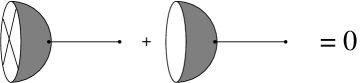
Figure 8: tadpole cancellation for one-loop

Eq.(3.37) reproduces the results stated in [45] and extend them to the presence of non-trivial open string moduli.

4 Unoriented one-loop amplitudes as analytic torsions

In this section we discuss B-model unorientable one-loop amplitudes for generic Calabi-Yau threefolds and provide a geometrical interpretation of them in terms of holomorphic torsions of appropriate vector bundles.

Let us consider the Klein bottle amplitude first. As we have already seen, this is given by the insertion of the involution operator ${\cal P}$ in the unoriented closed string trace as

$${\cal F}_{kle}=\int_{0}^{\infty}\frac{ds}{4s}{\rm Tr}_{{\cal H}_{c}}(-1)^{F}F{\cal P}e^{-2\pi sH_{c}}$$ (4.39)

which we can compute as follows. We recall from [4] that the closed topological string Hilbert space is given by ${\cal H}_{c}=\Lambda^{\bullet}TX\otimes\Lambda^{\bullet}\bar{T}^{*}X=\bigoplus_{p,q}\Lambda^{p}TX\otimes\Lambda^{q}\bar{T}^{*}X$, where $TX$ and $\bar{T}^{*}X$ denote the holomorphic tangent bundle and anti-holomorphic cotangent bundle respectively. At the level of the worldsheet superconformal field theory these spaces are generated by the zero modes of the $\eta^{\bar{I}}$ and $\theta_{I}=\theta^{\bar{I}}g_{\bar{I}I}$ fermions respectively. The parity ${\cal P}$ acts as ${\cal P}\eta^{\bar{I}}=\eta^{\bar{I}}$ and ${\cal P}\theta_{I}=-\theta_{I}$ [10]. It is thus clear that the projection operator acts as ${\cal P}=(-1)^{p}$ on the closed string Hilbert space. By inserting in (4.39) the expressions for the total fermion number $F=F_{L}+F_{R}=q-p$, a factor of $\frac{1}{2}$ which takes care of left/right identification and the closed string Hamiltonian in terms of the Laplacian $H=\Delta_{p,q}$, we get

$${\cal F}_{kle}=\frac{1}{8}\sum_{p,q}(-1)^{q}q~{}log\left({\det}^{\prime}\Delta_{p,q}\right)=-\frac{1}{4}\sum_{n}log{\rm T}\left(\Lambda^{n}\bar{T}^{*}X\right)=-\frac{1}{4}log{\rm T}\left(\Lambda^{\bullet}\bar{T}^{*}X\right)$$

in terms of the analytic Ray-Singer torsion ${\rm T}(V)$ of the bundle $V=\Lambda^{\bullet}\bar{T}^{*}X$.

The cylinder amplitude is given by

$${\cal F}_{cyl}=\int_{0}^{\infty}\frac{ds}{4s}{\rm Tr}_{{\cal H}_{o}}(-1)^{F}Fe^{-2\pi sH_{o}}$$

where the assignment of the Chan-Paton factors selects ${\cal H}_{o}=\oplus_{p}\Lambda^{p}TX\otimes E\otimes E^{*}$ and the Hamiltonian $H_{o}=\Delta_{p,E\otimes E^{*}}$ is the corresponding Laplacian. The result is (as already found in [4])

$${\cal F}_{cyl}=-\frac{1}{2}log{\rm T}\left(E\otimes E^{*}\right).$$

The last term to compute is the Möbius strip amplitude that is

$${\cal F}_{m\ddot{o}b}=\int_{0}^{\infty}\frac{ds}{4s}{\rm Tr}_{{\cal H}_{o}}(-1)^{F}F{\cal P}e^{-2\pi sH_{o}}$$

The only issue to discuss here is how to compute the trace with the ${\cal P}$ insertion. As explained in the appendix the trace over ${\cal P}$, for a $Sp(N/2)$ bundle, selects the $\textstyle{\rm{diag}}(E\otimes E)$ states with $-1$ eigenvalue. This is the only non trivial action of the ${\cal P}$ operator on the Hilbert space. Indeed, the boundary conditions project away the $\theta_{\bar{I}}$’s and we are left with the $\eta^{I}$’s only, on which ${\cal P}$ acts as the identity. Thus we get

$${\cal F}_{m\ddot{o}b}=+\frac{1}{2}log{\rm T}\left({\rm diag}(E\otimes E\right)).$$

Notice that the above conclusions agree with the explicit calculations of section 2, once restricted to the $T^{2}$ target space.

4.1 Wrong moduli independence and anomaly cancellation

In this section we show that the decoupling of wrong moduli in the unoriented open topological string on a Calabi-Yau threefold $X$ is equivalent to the usual D-brane/O-planes anomaly cancellation. This is performed for the B-model with a system of $N$ spacefilling D-branes. These are described by a Chan-Paton gauge bundle $E$ over $X$ with structure group $U(N)$. As it is well known however, in order to implement the orientifold projection, $E\sim E^{*}$ has to be real therefore reducing the structure group to $SO(N)$ or $Sp(N/2)$ if the fundamental representation is real or pseudo-real respectively.

Let us now calculate the variation of the unoriented topological string free energy at one loop under variations of the Kähler moduli. In order to do it, we use the Bismut formula [6] for the variation of the Ray-Singer torsion under a change of the base and fiber metrics $(g,h)\to(g+\delta g,h+\delta h)$

$$\left.\frac{1}{2\pi}\frac{\partial}{\partial t}\right|_{t=0}log{\rm T}(V)=\left.\frac{1}{2}\int_{X}\frac{\partial}{\partial t}\right|_{t=0}\left[Td\left(\frac{1}{2\pi}\left(iR+tg^{-1}\delta g\right)\right)Ch\left(\frac{1}{2\pi}\left(iF+th^{-1}\delta h\right)\right)\right]_{8}$$ (4.40)

By throwing the Bismut formula against the whole unoriented string free energy ${\cal F}^{u}_{\chi=0}={\cal F}_{cyl}+{\cal F}_{m\ddot{o}b}+{\cal F}_{kle}$ and specializing to the variations of the Kähler form only (that is at a fixed metric on the Chan-Paton holomorphic vector bundle) we get

$$\sim\int_{X}\left\{\left[(Ch(E))^{2}-n_{o}Ch({\rm diag}(E\otimes E))\right]\frac{\partial}{\partial t}[Td(TX)]_{t=0}+\frac{1}{2}n_{o}^{2}\frac{\partial}{\partial t}\left[Td(TX)Ch(\Lambda^{\bullet}T^{*})\right]_{t=0}\right\}$$ (4.41)

We will use $ch_{k}(2E)=2^{k}ch_{k}(E)$ and $ch_{k}(E^{*})=(-1)^{k}ch_{k}(E)$, so that for $E=E^{*}$, $ch_{k}(E)=0$ for $k$ odd. From the definitions

$$Td(TX)=\prod_{a}\frac{\gamma_{a}}{1-e^{-\gamma_{a}}}$$ (4.42)

$$Ch(\Lambda^{\bullet}T^{*}X)=\prod_{a}(1+e^{-\gamma_{a}})$$ (4.43)

we rewrite $Td(TX)=e^{c_{1}(T)/2}\hat{A}(TX)$ and $Td(TX)Ch(\Lambda^{\bullet}T^{*}X)=2^{3}L(TX)$. Using the standard expansions

$$\hat{A} = 1-\frac{2}{3}p_{1}2^{-4}+\frac{2}{45}\left(-4p_{2}+7p_{1}^{2}\right)2^{-8}+\ldots$$ (4.44)

$$L = 1+\frac{1}{3}p_{1}2^{-2}+\frac{1}{45}\left(7p_{2}-p_{1}^{2}\right)2^{-4}+\ldots$$

in (4.41) we calculate the variations of the cohomology classes above and obtain

$$\delta{\cal F}^{u}_{\chi=0}=\left.\int_{X}\sum_{i=1}^{2}C_{i}\frac{\partial}{\partial t}p_{i}\right|_{t=0}$$ (4.45)

with

$$C_{1} = -\frac{2^{-3}}{3}J_{4}(E)+\frac{2^{-6}\cdot 7}{45}p_{1}J_{0}(E)-\frac{2^{-1}}{45}n_{o}^{2}p_{1}$$ (4.46)

$$C_{2} = -\frac{2^{-5}}{45}J_{0}(E)+\frac{2^{-2}\cdot 7}{45}n_{o}^{2}$$ (4.47)

where $J(E)=(Ch(E))^{2}-n_{o}Ch({\rm diag}(E\otimes E))=J_{0}(E)+J_{4}(E)+\ldots$. One verifies that, setting $n_{o}=1$, the vanishing of the coefficients (4.46) and (4.47) is realized by

$$ch_{0}(E)=8$$ (4.48)

$$ch_{2}(E)=\frac{1}{4}p_{1}$$

that can be rewritten in the more familiar form

$$\sqrt{\hat{A}(TX)}Ch(E)-2^{3}\sqrt{\hat{L}(TX)}=0$$ (4.49)

that is the tadpole/anomaly cancellation condition for a system of spacefilling D-branes/O-planes on a Calabi-Yau threefold [32].

4.2 Quillen formula and holomorphic anomaly

In this subsection we compute the holomorphic anomaly equations of Section 3 from the expressions of the free energies in terms of Ray-Singer analytic torsion.

In order to do this, we apply the Quillen formula for torsions

$$\partial\bar{\partial}log[T(V)]=\partial\bar{\partial}\sum_{p}\frac{(-1)^{p+1}}{2}log[\det g^{(p)}_{V}]-\pi i\int_{X}\left[Td(TX)Ch(V)\right]_{(4,4)}$$ (4.50)

where $\det g^{(p)}_{V}$ is the volume element in the kernel of $\bar{\partial}_{V}$ on $\Lambda^{p}T^{*}X\otimes V$ and $V$ is the relevant vector bundle for each contribution (that is $V_{cyl}=E\otimes E$, etc. see the beginning of the section) comparing with the first and the last terms in the r.h.s. of formula (3.37).

In the notation of the previous subsection we get, up to the $\partial\bar{\partial}$-volume terms and setting $n_{o}=1$

$$\partial\bar{\partial}{\cal F}^{u}_{\chi=0}=-\frac{\pi i}{2}\int_{X}\left[Td(TX)J(E)+\frac{1}{2}Td(TX)Ch(\Lambda^{\bullet}T^{*}X)\right]_{(4,4)}+$$ (4.51)

$$+\frac{1}{4}\partial\bar{\partial}\left[\sum_{p}(-1)^{p}\left(log\left[\det g^{(p)}_{E\otimes E^{*}}\right]]-log\left[\det g^{(p)}_{diag(E\otimes E)}\right]+\frac{1}{2}log\left[\det g^{(p)}_{\Lambda^{\bullet}T^{*}X}\right]\right)\right]$$

which we can calculate using the expansions (4.1) for the vector bundle $E$ satisfying (4.1). The first line of (4.2) is

$$\pi i\int_{X}\left(\left(ch_{2}(E)\right)^{2}+\hat{A}_{4}\cdot 12ch_{2}(E)+7\cdot 8\hat{A}_{8}+4L_{8}\right)=0.$$ (4.52)

and vanishes. This result means that, once tadpoles are canceled, the $\bar{\Delta}\Delta$-term in (3.37) vanishes for spacefilling branes/orientifolds. This is in agreement with the result for $T^{2}$ target found in section 2.

5 Tadpole cancellation at all loops

5.1 Compactification of the moduli space of Riemann surfaces with boundaries

The moduli space of Klein surfaces with boundaries $\Sigma$ can be usefully described by referring to the notion of complex double $\left(\Sigma_{\mathbb{C}},\Omega\right)$, that is a compact orientable connected Riemann surface with an anti-holomorphic involution $\Omega$ (see figure 9).

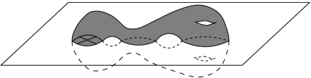
Figure 9: one example of an anti-holomorphic involution on $\Sigma$

The topological type of $\Sigma=\Sigma_{\mathbb{C}}/\Omega$ is classified by the fixed locus $\Sigma_{\mathbb{R}}$ of the involution [34]. If $\Sigma_{\mathbb{R}}=\emptyset$, then $\Sigma$ is non orientable and without boundaries, while if $\Sigma_{\mathbb{R}}$ is not empty, then $\Sigma$ has boundaries. In the latter case, $\Sigma$ is orientable if $\Sigma_{\mathbb{C}}\setminus\Sigma_{\mathbb{R}}$ is not connected and non orientable otherwise.

We recall that on a local chart $z\in{{\mathds{C}}}^{*}$, the anti-holomorphic involution acts as $\Omega_{\pm}(z)=\pm\frac{1}{\bar{z}}$. The involution $\Omega_{+}$ has a non empty fixed set with the topology of a circle, which after the quotient becomes a boundary component. The involution $\Omega_{-}$ doesn’t admit any fixed point and leads to a crosscap.

The compactification of the moduli space of open Klein surfaces can be studied from the point of view of the complex double [23]. In this context, the boundary is given as usual by nodal curves, but with respect to the closed orientable case there are new features appearing due to the quotient. In particular, nodes belonging to $\Sigma_{\mathbb{R}}$ can be smoothed either as boundaries or as crosscaps (see figure 10). Thus the moduli spaces of oriented and non orientable surfaces intersect at these boundary components of complex codimension one.

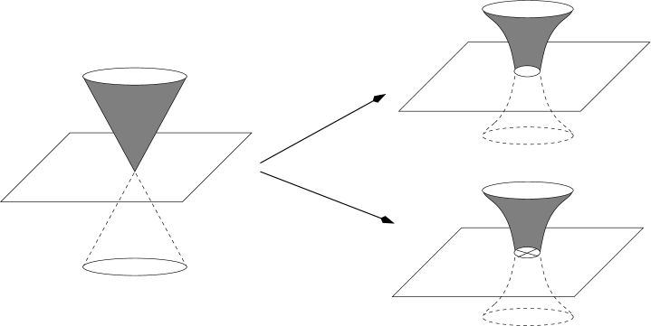
Figure 10: the complete resolution of a cone singularity in the doubling space

Actually there are also boundary components of real codimension one which are obtained when the degenerating 1-cycle of the complex double intersects $\Sigma_{\mathbb{R}}$ at points. In this cases, one obtains the boundary open string degenerations as described in [8]. The resolution of the real boundary nodes can be performed either as straight strips or as twisted ones. For example, when we have colliding boundaries, their singularity can be resolved either as splitting in two boundary components or as splitting in a single boundary and a crosscap (see figure 11). Thus the moduli space of oriented and unoriented surfaces intersect also along these components. For a more detailed and systematic description, see [28].

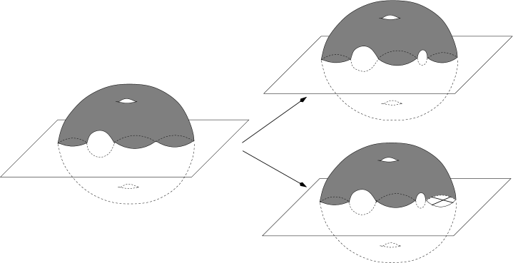
Figure 11: the resolution of a pinching point in the doubling space

More precisely, as discussed also in [7], the moduli space of the quotient surface $\Sigma$ is obtained by considering the relative Teichmüller space $T(\Sigma_{\mathds{C}},\Omega)$, that is the $\Omega$-invariant locus of $T(\Sigma_{\mathds{C}})$, modding the large diffeomorphisms $\Gamma(\Sigma_{\mathds{C}},\Omega)$ which commute with the involution $\Omega$

$${\cal M}_{\Sigma}=T(\Sigma_{\mathds{C}},\Omega)/\Gamma(\Sigma_{\mathds{C}},\Omega)$$ (5.53)

Let us consider as an example the case of null Euler characteristic. In this case the complex double is a torus and the annulus, Möbius strip and Klein bottle can be obtained by quotienting different anti-holomorphic involutions. The conformal families of tori admitting such involutions are Lagrangian submanifolds in the Teichmüller space of the covering torus modded by the translations $\tau\to\tau+1$ $\left\{\tau\in{\mathds{C}}|Im(\tau)>0,-\frac{1}{2}\leq Re(\tau)\leq\frac{1}{2}\right\}$. These are vertical straight lines at $Re(\tau)=0$ for the annulus and the Klein bottle while at $Re(\tau)=\pm\frac{1}{2}$ for the Möbius strip (see figure 12). Notice that all vertical lines meet at $\tau=i\infty$ which is the intersection point of the different moduli spaces.

\psfrag{tau}{$\tau$}\includegraphics[width=140.84256pt]{Techumuler}

Figure 12: different involutions represent in the moduli space of Torus

At a more general level, one should similarly discuss the moduli space of holomorphic maps from the worldsheet $\Sigma$ to the Calabi-Yau space $X$ with involution $\sigma$ in terms of equivariant maps $(\Sigma_{\mathbb{C}},\Omega)\to(X,\sigma)$ [23]. The above discussion suggests that the proper definition of open topological strings can be obtained by summing over all possible inequivalent involutions of $\Sigma_{\mathbb{C}}$. In particular one should include the contribution of non-orientable surfaces in order to have a natural definition of the compactification of the space of stable maps. Actually, once the perturbative expansion of the string amplitudes is set in terms of the Euler characteristic of the worldsheet, we have to sum over all possible contributions ${\cal F}_{\chi}=\sum_{g,h,c|\chi=2-2g-h-c}{\cal F}_{g,h,c}$ at given genus $g\geq 0$, boundary number $h\geq 0$ and crosscaps number $0\leq c\leq 2$.

At fixed Euler characteristic, the set of Riemann surfaces admitting an anti-holomorphic involution is a Lagrangian submanifold $L_{\Omega}$ of the Teichmüller space of the complex double $T_{\Sigma_{\mathbb{C}}}$ as in formula (5.53). Actually it might happen that the same Lagrangian submanifold corresponds to Riemann surfaces admitting inequivalent involutions which have to be counted independently, as for the example of the annulus and Klein bottle that we just discussed. The complete amplitude is then given schematically as

$${\cal F}^{u}_{\chi}=\sum_{\Omega}\int_{T_{\Sigma_{\mathbb{C}}}}\delta(L_{\Omega})\int_{\{\phi:\Sigma\to X,\phi\circ\Omega=\sigma\circ\phi\}}|\mu G^{-}|^{3\chi}$$

which provides a path integral representation for open/unoriented topological string amplitudes.

The above is the counterpart in topological string of the well-known fact that in open superstring theory unoriented sectors are crucial in order to obtain a consistent (i.e. tadpole and anomaly free) theory at all loops [5]. Evidence of these requirements has been found from a computational point of view in [45] where the contribution of unoriented surfaces has been observed to be necessary to obtain integer BPS counting formulas for A-model open invariants on some explicit examples. Let us remark that this picture applies to any compact or non compact Calabi-Yau threefold in principle. It might happen, however, that in the non compact case for some specific D-brane geometries tadpole cancellation can be ensured by choosing suitable boundary conditions at infinity so that the orientable theory is consistent by itself as in the case of [23, 42].

5.2 Local tadpole cancellation and holomorphic anomaly

As we have seen in the Section 5.1, non-orientable Riemann surfaces should be included in order to provide a consistent compactification of the moduli space of open strings. It was found in [12] that a dependence on wrong moduli appears when one considers holomorphic anomaly equations for orientable Riemann surfaces with boundaries. However, it follows from the discussion of Section 5.1 that whenever we consider a closed string degeneration in which one of the boundaries shrinks, there is always a corresponding component in the boundary of the complete moduli space where one crosscap is sent to infinity. Therefore, we always have this type of degeneration

$${\cal A}^{a}(\langle\omega_{a}|B\rangle+\langle\omega_{a}|C\rangle),$$ (5.54)

where $|B\rangle$ and $|C\rangle$ are the boundary and crosscap state respectively, $\omega_{a}$ is the operator inserted in the degenerated point which corresponds to a wrong modulus, ${\cal A}^{a}$ is the amplitude of the remaining Riemann surface with a wrong moduli operator insertion. Tadpole cancellation implies

$$\langle\omega_{a}|B\rangle+\langle\omega_{a}|C\rangle=0.$$ (5.55)

which ensures the cancellation of the anomaly of [12] at all genera. This cancellation has a simple geometrical interpretation in the A-model: in this case, we can have D6-branes and O6-planes wrapping 3-cycles of the Calabi-Yau 3-fold $X$, and the condition (5.55) reads

$$\langle\omega_{a}|B\rangle+\langle\omega_{a}|C\rangle=\partial_{y^{a}}\left(\int_{L}\Omega^{(3,0)}+\int_{X^{\sigma}}\Omega^{(3,0)}\right)=0,$$ (5.56)

where $L$ is a Lagrangian 3-cycle, $\Omega^{(3,0)}$ is the holomorphic 3-form, and $X^{\sigma}$ is the fixed point set of the involution $\sigma:X\rightarrow X$. From (5.56) we can interpret the local cancellation of the wrong moduli dependence (5.54) as a stability condition for the vacuum against wrong moduli deformations.

6 Conclusions

In this paper we discussed the issue of tadpole cancellation in the context of unoriented topological strings, and showed from Super Conformal Field Theory arguments that this corresponds to the decoupling of wrong moduli at all loops. We also provided a geometrical interpretation for unoriented B-model amplitudes at one loop in terms of analytic torsions of vector bundles over the target space.

Let us remark that the topological open A-model free energy is expected to provide a generating function for open Gromov-Witten invariants. However, these have not been defined rigorously yet, except for some particular cases [23, 17, 37]. We observe that the inclusion of unoriented worldsheet geometries turns out to be natural also from a purely mathematical viewpoint. In fact the compactified moduli spaces of open Riemann and Klein surfaces have common boundary components (see Section 5.1). Thus string theory suggests that a proper mathematical definition of open Gromov-Witten invariants should be obtained by including non-orientable domains for the maps. Therefore one should consider equivariant Gromov-Witten theory and sum over all possible involutions of the complex double, up to equivalences.

There are several interesting directions to be further investigated, the most natural being the study of holomorphic anomaly equations in presence of non-trivial open string moduli. This can be obtained by extending the holomorphic anomaly equations studied in [8] in order to include the contribution of non-orientable worldsheets.

Actually, our method is applicable only to cases in which the D-brane/orientifold set is modeled on the fixed locus of a target space involution. It would be quite interesting to be able to generalize it to a more general framework, that is to remove the reference to a given target space involution to perform the orientifold projection, in order to compare with some of the compact examples studied in [22, 18, 27, 46, 24].

It would be also interesting to link our B-model torsion formulae to the A-model side where open strings on orientifolds have been understood quite recently [30] to be the dual of coloured polynomials in the Chern-Simons theory. This should also enter a coloured extension of the conjecture stated in [14]. Notice also that interpretation of open B-model one loop amplitudes in terms of analytic torsions could be extended to more general target space geometries. For example one could investigate whether the notion of twisted torsions introduced in [41, 31] could provide a definition of B-model one loop amplitudes in the presence of $H$-fluxes and more in general with a target of generalized complex type. In such a context, our approach should lead to a generalization to open strings of the computation of exact gravitational threshold corrections as in [15, 19].

Acknowledgments: We thank A. Brini, R. Cavalieri, S. Cecotti, H.-L. Chang, J. Evslin, H. Liu, H. Ooguri, J. Walcher and J.-Y. Welschinger for discussions and exchange of opinions. We thank S. Natanzon for providing a copy of [34].

Appendix

Here we want to discuss in more detail the effect of the Chan-Paton factors to the amplitudes. The notation follows from [39]. An open string state is generalized carrying two indices at the two ends, each one running on the integers from $1$ to $N$. This additional state is indicated as $\left|i,j\right\rangle$ $(i,j=1...N)$.

The worldsheet parity $\Omega$ is defined to act exchanging $i$ with $j$ and rotating them with a $U(N)$ transformation $\gamma$. This rotation is added simply because it is still a symmetry for the amplitudes. Thus we have

$$\Omega\left|i,j\right\rangle\equiv\gamma_{j\>l}\left|l,k\right\rangle\gamma^{-1}_{k\>i}$$ (6.57)

Asking $\Omega^{2}=1$ [39] means requiring

$$\gamma^{T}=\pm\gamma$$ (6.58)

Now if we do a base change of the kind $\left|i,j\right\rangle\rightarrow\left|i^{\prime},j^{\prime}\right\rangle=U^{-1}_{i^{\prime}\>k}\left|k,l\right\rangle U_{l\>j^{\prime}}$ it transforms $\gamma$ in the new primed base so that $\gamma\rightarrow U^{T}\gamma U$. In particular choosing an appropriate $\left|i^{\prime},j^{\prime}\right\rangle$ base one can always transform $\gamma$ so that

$$\gamma=1\>\>\>\>\>or\>\>\>\>\>\gamma=\left(\begin{array}[]{cc}0&i\\ -i&0\end{array}\right)$$ (6.59)

respectively in the $+$ or $-$ case of (6.58). We start from the first case. There we can create the new base $\left|a\right\rangle=\Lambda^{a}_{i\>j}\left|i,j\right\rangle$ using $N^{2}$ independent matrices, in our case the $N\times N$ real matrices. Worldsheet parity action on the states $\left|a\right\rangle$ can be seen as an action on the coefficient $\Lambda^{a}_{i\>j}$. Choosing them either symmetric or antisymmetric one has respectively $\frac{1}{2}(N^{2}+N)$ and $\frac{1}{2}(N^{2}-N)$ of them. Since massless states transform with a minus under worldsheet parity, in order to create unoriented states one needs to couple these to Chan-Paton states $\left|a\right\rangle$ with antisymmetric coefficients. So a double minus gives a plus. Then the gauge field background, associated with those vertex operators, will be with values in the Lie Algebra of $N\times N$ anti-symmetric real matrices, that is $SO(N)$. From the spacetime effective action, with gauge field and matter in the adjoint, one has that the coupling of an $\left|a\right\rangle$ state with a generic background $A=A_{b}\Lambda^{b}$ is of the kind $\left[\Lambda^{a},A_{b}\Lambda^{b}\right]$. If the background is diagonal with elements $a_{1}...a_{N}$ and we consider the state $\left|a\right\rangle=\left|i,j\right\rangle$ this coupling gives an eigenvalue $+a_{i}-a_{j}$: the state $\left|i,j\right\rangle$ will shift the spacetime momenta as $p\rightarrow p+a_{i}-a_{j}$. This effect is more precisely described changing the string action with the addition of a gauge field background, which will manifest itself inserting in the path integral a Wilson loop of the kind

$$\prod_{k}{\rm Tr}e^{i\int_{\partial\Sigma_{k}}A_{\mu}\dot{X}^{\mu}}$$ (6.60)

where the sum is other all the connected components of the boundary. If one creates an open string state with a vertex operator on a boundary with non trivial homology, the left $i$ Chan-Paton sweeps in space giving an Aharonov-Bohm phase (6.60) $a_{i}$. The right $j$ Chan-Paton moves in the opposite direction on the same boundary and couples with a minus. For loop states with one Chan-Paton on a boundary and the second on another the situation is the same, always with one Chan-Paton moving along the orientation of the boundary and the other in the opposite .

Now for any (constant) $SO(N)$ background one can always act with a rigid gauge transformation to put it in the form

$$\bigoplus_{i}a_{i}\left(\begin{array}[]{cc}0&1\\ -1&0\end{array}\right)$$ (6.61)

This is still $SO(N)$ so the worldsheet parity still acts simply exchanging the $i-j$ factors. If in addition one wants to diagonalize it one needs to act with a gauge transformation that will change the $SO(N)$ form and so will have effects also on the shape of $\Omega$. In fact we can rewrite $\left|i,j\right\rangle=U_{i\>k^{\prime}}\left|k^{\prime},l^{\prime}\right\rangle U^{-1}_{l^{\prime}\>j}$ so that

$$\left|a\right\rangle=\Lambda^{a}_{i\>j}U_{i\>k^{\prime}}\left|k^{\prime},l^{\prime}\right\rangle U^{-1}_{l^{\prime}\>j}=U^{T}_{k^{\prime}\>i}\Lambda^{a}_{i\>j}(U^{\dagger})^{T}_{j\>l^{\prime}}\left|k^{\prime},l^{\prime}\right\rangle$$

This in order to transform $\Lambda^{a}$ so to diagonalize our background. But, acting in this way, the base $\left|i,j\right\rangle$ has changed and then also the worldsheet parity (6.57) will be different. In particular

$$\gamma(=I)\rightarrow U^{T}\gamma U(=U^{T}U)$$

When (6.61) is reduced to the simple two dimensional case the matrix $U^{T}$ which diagonalizes $A$ and $\gamma$ ( in the primed base ) are

$$U^{T}=\left(\begin{array}[]{cc}i/\sqrt{2}&1/\sqrt{2}\\ -i/\sqrt{2}&1/\sqrt{2}\end{array}\right)\>\>\>\>\>\>\gamma=\left(\begin{array}[]{cc}0&1\\ 1&0\end{array}\right)$$

The computation of the cylinder is straightforward. We have to sum over all states, and different Chan-Paton indices will modify the Hamiltonian with the usual momentum shift. Instead if we want to compute the Möbius strip we should look for diagonal states of $\Omega$. It is easy to see that, in the $\left|i^{\prime},j^{\prime}\right\rangle$ base, they are $\left|1,2\right\rangle$ and $\left|2,1\right\rangle$, both with eigenvalue $+1$. Each diagonal term in the trace will contribute both with its eigenvalue and with its own Hamiltonian. In our case the two states will change the momenta respectively as $p\rightarrow p+a_{1}-a_{2}$ and $p\rightarrow p+a_{2}-a_{1}$ where, for our diagonalized $SO(2)$ background, $a_{1}=ia$ and $a_{2}=-ia$. Generalization to higher $N$ is straightforward. Then we end up with our amplitudes.

The $Sp(N/2)$ situation is even simpler. There the diagonal background is already an $Sp(N/2)$ algebra matrix if in the form

$$\textstyle{\rm{diag}}\{a_{1},\cdots,a_{N/2},-a_{1},\cdots,-a_{N/2}\}$$

Therefore the worldsheet parity $\Omega$ is still the second of (6.59). Diagonal states are now $\left|i,i+N/2\right\rangle$ or $\left|i+N/2,i\right\rangle$ for $i=1...N/2$, note both with negative eigenvalues. The contribution to the Hamiltonian is again $p\rightarrow p\pm 2a_{i}$.

References

- [1] B. S. Acharya, M. Aganagic, K. Hori and C. Vafa, “Orientifolds, mirror symmetry and superpotentials,” arXiv:hep-th/0202208.
- [2] I. Antoniadis, E. Gava, K. S. Narain and T. R. Taylor, “Topological amplitudes in string theory,” Nucl. Phys. B 413 (1994) 162 [arXiv:hep-th/9307158].
- [3] I. Antoniadis, K. S. Narain and T. R. Taylor, “Open string topological amplitudes and gaugino masses,” Nucl. Phys. B 729 (2005) 235 [arXiv:hep-th/0507244].
- [4] M. Bershadsky, S. Cecotti, H. Ooguri and C. Vafa, “Kodaira-Spencer theory of gravity and exact results for quantum string amplitudes,” Commun. Math. Phys. 165 (1994) 311 [arXiv:hep-th/9309140].
- [5] M. Bianchi and A. Sagnotti, “The partition function of the SO(8192) bosonic string,” Phys. Lett. B 211 (1988) 407.
- [6] J. Bismut, H. Gillet, C. Soulé, “Analytic torsion and holomorphic determinant bundles. III. Quillen metrics on holomorphic determinants,” Comm. Math. Phys. 115 (1988), no. 2, 301.
- [7] S. Blau, M. Clements, S. Della Pietra, S. Carlip and V. Della Pietra, “The String Amplitude On Surfaces With Boundaries And Crosscaps,” Nucl. Phys. B 301 (1988) 285.
- [8] G. Bonelli and A. Tanzini, “The holomorphic anomaly for open string moduli,” JHEP 0710 (2007) 060 [arXiv:0708.2627 [hep-th]].
- [9] V. Bouchard, B. Florea and M. Marino, “Counting higher genus curves with crosscaps in Calabi-Yau orientifolds,” JHEP 0412 (2004) 035 [arXiv:hep-th/0405083]; V. Bouchard, B. Florea and M. Marino, “Topological open string amplitudes on orientifolds,” JHEP 0502 (2005) 002 [arXiv:hep-th/0411227].
- [10] I. Brunner and K. Hori, “Orientifolds and mirror symmetry,” JHEP 0411 (2004) 005 [arXiv:hep-th/0303135].
- [11] A. Collinucci, P. Soler, A.M. Uranga, “Non-perturbative effects and wall-crossing from topological strings”, arXiv:0904.1133 [hep-th].
- [12] P. Cook, H. Ooguri, and J. Yang, “ New Anomalies in Topological String Theory,” arXiv:0804.1120 [hep-th].
- [13] D. E. Diaconescu, B. Florea and A. Misra, “Orientifolds, unoriented instantons and localization,” JHEP 0307 (2003) 041 [arXiv:hep-th/0305021].
- [14] R. Dijkgraaf and H. Fuji, “The Volume Conjecture and Topological Strings,” arXiv:0903.2084 [hep-th].
- [15] S. Ferrara, J. A. Harvey, A. Strominger and C. Vafa, “Second Quantized Mirror Symmetry,” Phys. Lett. B 361 (1995) 59 [arXiv:hep-th/9505162].
- [16] D. Gaiotto, G. W. Moore and A. Neitzke, “Four-dimensional wall-crossing via three-dimensional field theory,” arXiv:0807.4723 [hep-th].
- [17] T. Graber and E. Zaslow, “Open string Gromov-Witten invariants: Calculations and a mirror ’theorem’,” arXiv:hep-th/0109075.
- [18] T. W. Grimm, T. W. Ha, A. Klemm and D. Klevers, “The D5-brane effective action and superpotential in N=1 compactifications,” arXiv:0811.2996 [hep-th].
- [19] J. A. Harvey and G. W. Moore, “Exact gravitational threshold correction in the FHSV model,” Phys. Rev. D 57 (1998) 2329 [arXiv:hep-th/9611176].
- [20] F. Hirzebruch, “ Topological Methods in Algebraic Geometry,” Springer-Verlag 1978.
- [21] D. L. Jafferis and G. W. Moore, “Wall crossing in local Calabi Yau manifolds,” arXiv:0810.4909 [hep-th].
- [22] H. Jockers and M. Soroush, “Relative periods and open-string integer invariants for a compact Calabi-Yau hypersurface,” arXiv:0904.4674 [hep-th].
- [23] S. Katz and C. Liu, “Enumerative Geometry of Stable Maps with Lagrangian Boundary Conditions and Multiple Covers of the Disc,” Adv. Theor. Math. Phys. 5 (2002) 1 [arXiv:math/0103074].
- [24] J. Knapp and E. Scheidegger, “Towards Open String Mirror Symmetry for One-Parameter Calabi-Yau Hypersurfaces,” arXiv:0805.1013 [hep-th].
- [25] M. Kontsevich, and Y. Soibelman “Stability structures, motivic Donaldson-Thomas invariants and cluster transformations ,“ arXiv:0811.2435 [math.AG].
- [26] D. Krefl and J. Walcher, “The Real Topological String on a local Calabi-Yau,” arXiv:0902.0616 [hep-th].
- [27] D. Krefl and J. Walcher, “Real Mirror Symmetry for One-parameter Hypersurfaces,” JHEP 0809 (2008) 031 [arXiv:0805.0792 [hep-th]].
- [28] C. Liu, “Moduli of J-Holomorphic Curves with Lagrangian Boundary Conditions and Open Gromov-Witten Invariants for an -Equivariant Pair,” arXiv:math/0210257.
- [29] M. Marino, “Nonperturbative effects and nonperturbative definitions in matrix models and topological strings,” JHEP 0812 (2008) 114 [arXiv:0805.3033 [hep-th]]; M. Marino, R. Schiappa and M. Weiss, “Nonperturbative Effects and the Large-Order Behavior of Matrix Models and Topological Strings,” arXiv:0711.1954 [hep-th]; M. Marino, R. Schiappa and M. Weiss, “Multi-Instantons and Multi-Cuts,” arXiv:0809.2619 [hep-th].
- [30] M. Marino, “String theory and the Kauffman polynomial”, arXiv:0904.1088 [hep-th].
- [31] V. Mathai, and S. Wu, “Analytic torsion for twisted de Rham complexes” arXiv:0810.4204 [math.DG].
- [32] J. Morales, C. Scrucca and M. Serone, “Anomalous couplings for D-branes and O-planes,” Nucl. Phys. B 552 (1999) 291 [arXiv:hep-th/9812071]; B. Stefanski, “Gravitational couplings of D-branes and O-planes,” Nucl. Phys. B 548 (1999) 275 [arXiv:hep-th/9812088]; C. Scrucca and M. Serone, “Anomalies and inflow on D-branes and O-planes,” Nucl. Phys. B 556 (1999) 197 [arXiv:hep-th/9903145].
- [33] K. Nagao and H. Nakajima, “Counting invariant of perverse coherent sheaves and its wall-crossing ” arXiv:0809.2992 [math.AG].
- [34] S. Natanzon, “Moduli space of real curves,” Trans. Moscow Math. Soc. 1 (1980) 233; “Finite groups of homeomorphisms of surfaces and real forms of complex algebric curves,” Trans. Moscow Math. Soc. 51 (1989) 1; “Klein surfaces,” Rus. Math. Sur 46:6 (1990) 53; “Moduli of Riemann surfaces, real algebraic curves, and their superanalogs,” Translations of Math. Monographs v. 225 Amer. Math. Soc.
- [35] H. Ooguri, Y. Oz and Z. Yin, “D-branes on Calabi-Yau spaces and their mirrors,” Nucl. Phys. B 477 (1996) 407 [arXiv:hep-th/9606112].
- [36] H. Ooguri and M. Yamazaki, “Emergent Calabi-Yau Geometry,” arXiv:0902.3996 [hep-th].
- [37] R. Pandharipande, J. Solomon and J. Walcher, “Disk enumeration on the quintic 3-fold,” arXiv:math/0610901.
- [38] V. Pestun and E. Witten, “The Hitchin functionals and the topological B-model at one loop,” Lett. Math. Phys. 74 (2005) 21 [arXiv:hep-th/0503083].
- [39] J. Polchinski, “String theory,” Vol 1, Cambridge University Press 2001.
- [40] D. Ray and I. Singer, “ Analytic torsion for complex manifolds,” Ann. Math. 98 (1973) 154.
- [41] R. Rohm and E. Witten, “The Antisymmetric Tensor Field In Superstring Theory,” Annals Phys. 170 (1986) 454.
- [42] S. Sinha and C. Vafa, “SO and Sp Chern-Simons at large N,” arXiv:hep-th/0012136.
- [43] C. Vafa, “Extending mirror conjecture to Calabi-Yau with bundles,” arXiv:hep-th/9804131.
- [44] J. Walcher, “Extended Holomorphic Anomaly and Loop Amplitudes in Open Topological String,” arXiv:0705.4098 [hep-th].
- [45] J. Walcher, “Evidence for Tadpole Cancellation in the Topological String,” arXiv:0712.2775 [hep-th].
- [46] J. Walcher, “Calculations for Mirror Symmetry with D-branes,” arXiv:0904.4905 [hep-th].
- [47] E. Witten, “Mirror manifolds and topological field theory,” arXiv:hep-th/9112056.