Increasing the sensitivity of future gravitational-wave detectors with double squeezed-input

Abstract

We consider improving the sensitivity of future interferometric gravitational-wave detectors by simultaneously injecting two squeezed vacuums (light), filtered through a resonant Fabry-Perot cavity, into the dark port of the interferometer. The same scheme with single squeezed vacuum was first proposed and analyzed by Corbitt et al. Corbitt . Here we show that the extra squeezed vacuum, together with an additional homodyne detection suggested previously by one of the authors Khalili1 , allows reduction of quantum noise over the entire detection band. To motivate future implementations, we take into account a realistic technical noise budget for Advanced LIGO (AdvLIGO) and numerically optimize the parameters of both the filter and the interferometer for detecting gravitational-wave signals from two important astrophysics sources, namely Neutron-Star–Neutron-Star (NSNS) binaries and Bursts. Assuming the optical loss of the $\sim 30$m filter cavity to be $10$ppm per bounce and 10dB squeezing injection, the corresponding quantum noise with optimal parameters lowers by a factor of 10 at high frequencies and goes below the technical noise at low and intermediate frequencies.

I Introduction

During the last decade, several laser interferometric gravitational-wave detectors including LIGO LIGO , VIRGO VIRGO , GEO600 GEO and TAMA TAMA have been built and operated almost at their design sensitivity, aiming at extracting gravitational-wave signals from various astrophysical sources. At present, developments of next-generation detectors such as AdvLIGO AdvLIGO are also under way, and sensitivities of these advanced detectors are anticipated to be limited by quantum noise nearly over the whole observational band from $10$ Hz to $10^{4}$ Hz. At high frequencies, the dominant quantum noise is photon shot noise, caused by phase fluctuation of the optical field; while at low frequencies, the radiation-pressure noise, due to the amplitude fluctuation, dominates and it exerts a noisy random force on the probe masses. These two noises, if uncorrelated, will impose a lower bound on the noise spectrum, which is called the Standard Quantum Limit (SQL). In terms of gravitational-wave strain $h\equiv\Delta L/L$, it is given by

$$S_{h}^{\rm SQL}=\frac{8\hbar}{m\,\Omega^{2}L^{2}}.$$ (1)

It can also be derived from the fact that position measurements of the free test mass do not commute with themselves at different time Thorne .

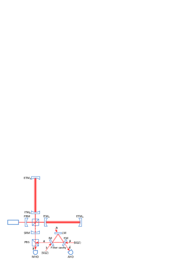
Figure 1: Schematic plot of the proposed configuration. Two squeezed vacuums $\hat{\textbf{{s}}},\hat{\textbf{{p}}}$ are injected from both side of the filter cavity rather than the one which was considered in Refs. Corbitt ; Khalili1 . The signal is detected by the main homodyne detector (MHD) and additional detector (AHD) is made in the idle port of the filter cavity.

The existence of SQL was first realized by Braginsky in 1960’s Braginsky1 ; Braginsky2 . Since then, various approaches are proposed to beat the SQL. One recognized by Braginsky is to measure conserved quantities of the probe masses (also called quantum nondemolition quantities). This can be achieved, e.g. by adopting speed-meter configurations Khalili2 ; Braginsky3 ; Purdue1 ; Purdue2 ; Yanbei ; Danilishin , which measure the conserved quantity – momentum rather than the position. An alternative is to change the dynamics of the probe mass, e.g. using optical rigidity Braginsky4 ; Khalili3 , in which case the free mass SQL mentioned is no longer relevant. As shown by Buonanno and Chen Buonanno1 ; Buonanno2 ; Buonanno3 , optical rigidity exists in signal-recycled (SR) interferometric gravitational-wave detectors; therefore we can beat the SQL without radical redesigns of existing topology of the interferometers. Another approach is to modify input and/or output optics of the interferometers such that photon shot noise and radiation-pressure noise are correlated. After the initial paper by Unruh Unruh1982 , this was further developed by other authors 87a1eKh ; JaekelReynaud1990 ; Pace1993 ; Vyatchanin ; Kimble ; Buonanno4 ; Corbitt ; Arcizet2006 ; 06a2Kh . A natural way to achieve this is injecting squeezed vacuum, whose phase and amplitude fluctuations are correlated, into the dark port of the interferometers. With great advancements in preparation of the squeezed state McKenzie ; Vahlbruch , squeezed-input interferometers will be promising candidates for third-generation gravitational-wave detectors. As elaborated in the work of Kimble et al. Kimble , frequency-dependent squeezing is essential to reduce the quantum noise at various frequencies of the observation band. In addition, they demonstrated that this can be realized by filtering the frequency-independent squeezed vacuum through two detuned Fabry-Perot cavities before sending into the interferometer. Their results were extended by Buonanno and Chen Buonanno4 where the filters for general cases were discussed.

Another method, which also uses an additional filter cavity and squeezed light, but in a completely different way, was proposed by Corbitt, Mavalvala, and Whitcomb (hereafter referred as CMW) Corbitt . They proposed to use a tuned optical cavity as a high-pass filter for the squeezed vacuum. This scheme does not create the noises correlation, but instead, renders the noises spectral densities frequency dependent. At high frequencies, the phase squeezed vacuum gets reflected by the filter and enters the interferometer such that high-frequency shot noise is reduced; while at low frequencies, ordinary vacuum transmits through the filter and enters the interferometer, thus low-frequency radiation-pressure noise remains unchanged. One significant advantage is that the squeezed vacuum does not really enter the filter cavity and thus it is less susceptible to the optical losses. However, it does not perform so well as hoped for, and there is a noticeable degradation of sensitivity in the intermediate-frequency range. One of us – Khalili Khalili1 pointed out that this has to do with the quantum entanglement between the optical fields at two ports of the filter cavity. Equivalently, it can be interpreted physically as the following: some information about phase and amplitude fluctuation flows out from the idle port of the filter cavity and the remaining quantum state which enters the interferometer is not pure. In order to recover the sensitivity, the filter cavity needs to have a low optical loss such that these information can be collected with an additional homodyne detector (AHD) at the idle port. Given an achievable optical loss of the filter cavity $\sim 10$ppm per bounce, Khalili showed that we can obtain the desired sensitivity at intermediate frequencies. A natural extension of this scheme is sending additional squeezed vacuum into the idle port of the filter cavity such that the low-frequencies radiation-pressure noise is also suppressed. The corresponding configuration is shown schematically in Fig. 1, where two squeezed vacuums $\hat{\textbf{{s}}}$ and $\hat{\textbf{{p}}}$ are injected from two ports of the filter cavity, and some ordinary vacuum $\hat{\textbf{{n}}}$ leaks into the filter due to optical losses. By optimizing the squeezing angles of squeezed states, we will show that the resulting quantum noise is reduced over the entire observational band.

The outline of this paper is as follows. In Sec. II, we will calculate the quantum noises in this double squeezed-input CMW scheme with AHD (later referred as CMWA). We will use the same notation as in Ref Buonanno3 , which enables us to extend the results in Ref. Khalili1 to the case of signal-recycled interferometers easily. In Sec. III, we numerically optimize the parameters of this new scheme for searching the gravitational-wave signals from NSNS binaries and Bursts. Finally, we will summarize our results in Sec. IV. For simplicity, we will neglect the optical losses inside the main interferometer, but we consider the losses from the filter cavity and also non-unity quantum efficiency of the photodiodes. The losses from the main interferometer are not expected to be important as shown in Refs. Kimble ; Buonanno1 ; Khalili4 . The main notations used in this paper are listed in Table 1.

Table 1: Main notations used in this paper.

Quantity	Value for Estimates	Descriptions
$\Omega$		Gravitational wave (sideband) frequency
$c$	$3.0\times 10^{8}$ m/s	Speed of light
$\omega_{0}$	$1.8\times 10^{15}~{}{\rm s}^{-1}$	Optical pumping frequency
$m$	40 kg	Mass of the end mirrors
$L$	4 km	Length of the arm cavity
$I_{c}$	840 kW	Circulating optical power
$\iota_{c}=\frac{8\omega_{0}I_{c}}{mLc}$	$(2\pi\times 100)^{3}{\rm s}^{-3}$
$\gamma_{\rm arm}$	$2\pi\times 100~{}{\rm s}^{-1}$	Bandwidth of the arm cavity
$r_{\rm SR}$		Amplitude reflectivity of the SRM
$\phi_{\rm SR}$		Phase detuning of the SR cavity
$\delta$		Effective frequency detuning of the SR interferometer
$\gamma$		Effective bandwidth of the SR interferometer
$\phi$		Homodyne angle of the MHD
$\zeta$		Homodyne angle of the AHD
$L_{f}$	30 m	Length of the filter cavity
$\gamma_{\rm\sf I,E,L}=\frac{T_{\rm\sf I,E,L}^{2}}{2\tau_{f}}$
$\gamma_{f}=\gamma_{\rm\sf I}+\gamma_{\rm\sf E}+\gamma_{\rm\sf L}$		Bandwidth of the filter cavity
$r_{i}~{}(i=s,p)$	$(\ln 10)/2\;$ (10dB)	Squeezing factors
$\theta_{i}~{}(i=s,p)$		Squeezing angles

II Quantum noise calculation

II.1 Filter cavity

In this section, we will derive single-sided spectral densities of the two outgoing fields $\hat{\textbf{{a}}}$ and $\hat{\textbf{{q}}}$ as shown in Fig. 1. From the continuity of optical fields, we can relate them to ingoing fields, which include two squeezed vacuums $\hat{\textbf{{s}}},~{}\hat{\textbf{{p}}}$ and one ordinary vacuum $\hat{\textbf{{n}}}$ entering from the lossy mirror (LM) Khalili1 . Specifically, we have

$$\hat{\textbf{{a}}}(\Omega) = {\cal R}_{\rm\sf I}(\Omega)\hat{\textbf{{s}}}(\Omega)+{\cal T}(\Omega)\hat{\textbf{{p}}}(\Omega)+{\cal A}_{\rm\sf I}(\Omega)\hat{\textbf{{n}}}(\Omega),$$ (2)

$$\hat{\textbf{{q}}}(\Omega) = {\cal R}_{\rm\sf E}(\Omega)\hat{\textbf{{p}}}(\Omega)+{\cal T}(\Omega)\hat{\textbf{{s}}}(\Omega)+{\cal A}_{\rm\sf E}(\Omega)\hat{\textbf{{n}}}(\Omega).$$ (3)

Here $\hat{\textbf{{a}}}=(\hat{a}_{A},~{}\hat{a}_{\varphi})^{\rm T}$, $\hat{\textbf{{q}}}=(\hat{q}_{A},~{}\hat{q}_{\varphi})^{\rm T}$ are amplitude and phase quadratures (subscript $A$ stands for amplitude and $\varphi$ for phase). In our case, the carrier light is resonant inside the filter cavity. Therefore, the effective amplitude reflectivity ${\cal R}$, transmissivity ${\cal T}$ and loss ${\cal A}$ can be written as,

$${\cal R}_{\rm\sf I}(\Omega) =\frac{\gamma_{\rm\sf I}-\gamma_{\rm\sf E}-\gamma_{\rm\sf L}+i\Omega}{\gamma_{f}-i\Omega}\,, {\cal R}_{\rm\sf E}(\Omega) =\frac{\gamma_{\rm\sf E}-\gamma_{\rm\sf I}-\gamma_{\rm\sf L}+i\Omega}{\gamma_{f}-i\Omega}\,,$$ (4a)

$${\cal T}(\Omega) =\frac{-2\sqrt{\gamma_{\rm\sf I}\gamma_{\rm\sf E}}}{\gamma_{f}-i\Omega},$$ (4b)

$${\cal A}_{\rm\sf I}(\Omega) =\frac{-2\sqrt{\gamma_{\rm\sf I}\gamma_{\rm\sf L}}}{\gamma_{f}-i\Omega}\,, {\cal A}_{\rm\sf E}(\Omega) =\frac{2\sqrt{\gamma_{\rm\sf E}\gamma_{\rm\sf L}}}{\gamma_{f}-i\Omega}\,$$ (4c)

where $\gamma_{f}\equiv\gamma_{\rm\sf I}+\gamma_{\rm\sf E}+\gamma_{\rm\sf L}$. They satisfy the following identities,

$$|{\cal R}_{\rm\sf I}(\Omega)|^{2}+|{\cal T}(\Omega)|^{2}+|{\cal A}_{\rm\sf I}(\Omega)|^{2}=|{\cal R}_{\rm\sf E}(\Omega)|^{2}+|{\cal T}(\Omega)|^{2}+|{\cal A}_{\rm\sf E}(\Omega)|^{2}=1,$$ (5a)

$${\cal R}^{*}_{\rm\sf I}(\Omega){\cal T}(\Omega)+{\cal R}_{\rm\sf E}(\Omega){\cal T}^{*}(\Omega)+{\cal A}^{*}_{\rm\sf I}(\Omega){\cal A}_{\rm\sf E}(\Omega)=0.$$ (5b)

If the input and end mirrors of the filter cavity are identical, namely $\gamma_{\rm\sf I}=\gamma_{\rm\sf E}$, we will have ${\cal R}_{\rm\sf I},{\cal R}_{\rm\sf E}\sim 1$ and ${\cal T}\sim 0$ when $\Omega\gg\gamma_{f}$ and ${\cal R}_{\rm\sf I},{\cal R}_{\rm\sf E}\sim 0$ and ${\cal T}\sim 1$ when $\Omega\ll\gamma_{f}$. Therefore, the squeezed vacuum $\hat{\textbf{{s}}}$ enters the interferometer at high frequencies while $\hat{\textbf{{p}}}$ becomes significant mostly at low frequencies. By adjusting the squeezing factor and angle of these two squeezed fields, we can reduce both the high-frequency shot noise and low-frequency radiation-pressure noise simultaneously.

To calculate the noise spectral densities, we assume these two squeezed vacuums have frequency-independent squeezing angles $\theta_{i}~{}(i=s,~{}p)$ and can be represented as follows:

$$\hat{\textbf{{s}}} =\widetilde{R}(r_{s},\theta_{s})\hat{\textbf{{v}}}_{s}\,, \hat{\textbf{{p}}} =\widetilde{R}(r_{p},\theta_{p})\hat{\textbf{{v}}}_{p}\,,$$ (6)

with

$$\widetilde{R}(r,\theta)\equiv\left(\begin{array}[]{cc}\cosh r-\cos\theta\sinh r&-\sin\theta\sinh r\\ -\sin\theta\sinh r&\cosh r+\cos\theta\sinh r\end{array}\right).$$ (7)

Here $r$ is the squeezing factor, and $\hat{\textbf{{v}}}_{i}=(\hat{v}_{iA},~{}\hat{v}_{i\varphi})^{\rm T}$ are ordinary vacuums with single-sided spectral densities: $S_{A}(\Omega)=S_{\varphi}(\Omega)=1,~{}~{}S_{A\varphi}(\Omega)=0$ Kimble .

The noise spectral densities of the two filter-cavity outputs can then be written as

$$\widetilde{S}_{\hat{a}\hat{a}}(\Omega) = |{\cal R}_{\rm\sf I}(\Omega)|^{2}\widetilde{R}(2r_{s},2\theta_{s})+|{\cal T}(\Omega)|^{2}\widetilde{R}(2r_{p},2\theta_{p})+|{\cal A}_{\rm\sf I}(\Omega)|^{2}\widetilde{\rm I},$$ (8)

$$\widetilde{S}_{\hat{q}\hat{q}}(\Omega) = |{\cal R}_{\rm\sf E}(\Omega)|^{2}\widetilde{R}(2r_{p},2\theta_{p})+|{\cal T}(\Omega)|^{2}\widetilde{R}(2r_{s},2\theta_{s})+|{\cal A}_{\rm\sf E}(\Omega)|^{2}\widetilde{\rm I},$$ (9)

$$\widetilde{S}_{\hat{a}\hat{q}}(\Omega) = {\cal R}_{\rm\sf E}(\Omega){\cal T}^{*}(\Omega)\widetilde{R}(2r_{p},2\theta_{p})+{\cal R}_{\rm\sf I}^{*}(\Omega){\cal T}(\Omega)\widetilde{R}(2r_{s},2\theta_{s})+{\cal A}_{\rm\sf E}(\Omega){\cal A}_{\rm\sf I}^{*}(\Omega)\widetilde{\rm I},$$ (10)

where $\widetilde{S}_{\hat{a}\hat{q}}(\Omega)$ is the cross correlation between two outputs; $\widetilde{\rm I}$ is the identity matrix and

$$\widetilde{S}_{i}(\Omega)=\left(\begin{array}[]{cc}S_{A,{i}}(\Omega)&S_{A\varphi,{i}}(\Omega)\\ S_{A\varphi,{i}}(\Omega)&S_{\varphi,{i}}(\Omega)\end{array}\right)$$ (11)

with $i=\hat{a}\hat{a},\hat{q}\hat{q},\hat{a}\hat{q}$, whose elements are single-sided spectral densities.

II.2 Quantum noise of the interferometer

According to Ref. Buonanno3 , the input-output relation, which connects ingoing fields $\hat{\textbf{{a}}}$ and gravitational-wave signal $h$ with the outgoing fields $\hat{\textbf{{b}}}$, for a signal-recycled interferometer can be written as

$$\hat{\textbf{{b}}}=\frac{1}{M}\left(\widetilde{C}~{}\hat{\textbf{{a}}}+{\bf D}~{}\frac{h}{h_{\rm SQL}}\right).$$ (12)

In the above equation,

$$M=[\delta^{2}-(\Omega+i\gamma)^{2}]\Omega^{2}-\delta\,\iota_{c},$$ (13)

and $\widetilde{C}$ is the transfer function matrix with elements

$$\widetilde{C}_{11} =\widetilde{C}_{22}=\Omega^{2}(\Omega^{2}-\delta^{2}+\gamma^{2})+\delta\,\iota_{c},$$ (14a)

$$\widetilde{C}_{12} =-2\gamma\,\delta\,\Omega^{2},~{}~{}~{}\widetilde{C}_{21}=2\gamma\,\delta\,\Omega^{2}-2\gamma\,\iota_{c},$$ (14b)

where $\iota_{c}\equiv 8\omega_{0}I_{c}/(m\,c\,L)$. The elements of the transfer function vector ${\bf D}$ are

$$D_{1} =-2\delta\sqrt{\gamma\,\iota_{c}}\,\Omega,~{}D_{2}=-2(\gamma-i\Omega)\sqrt{\gamma\,\iota_{c}}\,\Omega.$$ (15a)

The effective detuning $\delta$ and bandwidth $\gamma$ are given by

$$\delta =\frac{2\,r_{\rm SR}\,\gamma_{\rm arm}\sin(2\,\phi_{\rm SR})}{1+r_{\rm SR}^{2}+2\,r_{\rm SR}\cos(2\phi_{\rm SR})},$$ (16a)

$$\gamma =\frac{(1-r_{\rm SR}^{2})\gamma_{\rm arm}}{1+r_{\rm SR}^{2}+2\,r_{\rm SR}\cos(2\,\phi_{\rm SR})},$$ (16b)

where $r_{\rm SR}$ is the amplitude reflectivity of the signal recycling mirror ($\rm\sf SRM$) and $\phi_{\rm SR}$ is phase detuning of the SR cavity. If the main homodyne detector (MHD) measures

$$\hat{b}_{\phi}(\Omega)=\sqrt{\eta}\,[\sin\phi~{}\hat{b}_{A}(\Omega)+\cos\phi~{}\hat{b}_{\varphi}(\Omega)]+\sqrt{1-\eta}~{}\hat{v}(\Omega),$$ (17)

where $\phi$ is the homodyne angle and $\hat{v}$ is the additional vacuum due to non-unity quantum efficiency of the photodiode, and then the corresponding $h$-referred quantum-noise spectral density can be written as

$$S_{h}(\Omega)=h^{2}_{\rm SQL}\frac{(\sin\phi~{}\cos\phi)\widetilde{C}\,\widetilde{S}_{\rm\sf I}\,\widetilde{C}^{{\dagger}}(\sin\phi~{}\cos\phi)^{\rm T}+\frac{1-\eta}{\eta}|M|^{2}}{(\sin\phi~{}\cos\phi)\widetilde{D}\,\widetilde{D}^{{\dagger}}(\sin\phi~{}\cos\phi)^{\rm T}}.$$ (18)

It can be minimized by adjusting the squeezing angle $\theta$ of $\hat{\textbf{{s}}}$ and $\hat{\textbf{{p}}}$. We can estimate the optimal $\theta$ qualitatively from the asymptotic behavior of the resulting noise spectrum. At very high frequencies ($\Omega\gg\gamma$), from Eq. (2), $\hat{\textbf{{a}}}\sim\hat{\textbf{{s}}}$ and thus

$$S_{h}(\Omega)\propto\cosh(2r_{s})+\cos[2(\phi+\theta_{s})]\sinh(2r_{s}).$$ (19)

If the squeezing angle of $\hat{\textbf{{s}}}$

$$\theta_{s}=\frac{\pi}{2}+n\pi-\phi$$ (20)

where $n$ is integer, we achieve the optimal case, namely $S_{h}\propto e^{-2r_{s}}$. Similarly, at very low frequencies ($\Omega\ll\gamma$), we have $\hat{\textbf{{a}}}\sim\hat{\textbf{{p}}}$ and the spectral density $S_{h}\propto e^{-2r_{p}}$ if

$$\theta_{p}=\arctan\left[\frac{2\cos\phi\sin\beta}{\cos(\beta-\phi)+3\cos(\beta+\phi)}\right].$$ (21)

More accurate values for optimal $\theta_{s,p}$ can be obtained numerically as we will apply in the next section. Given optimal $\theta_{s,p}$, the sensitivity of this double squeezed-input scheme improves at both high and low frequencies. However, due to the same reason as in the case of single squeezed-input that two outputs of the filter cavity are entangled Khalili1 , this double squeezed-input scheme does not perform well in the intermediate frequency range. To recover the sensitivity, we need to use an additional homodyne detector (AHD) at the idle port E of the filter cavity. The corresponding measured quantity is

$$\hat{q}_{\zeta}(\Omega)=\sqrt{\eta}\,[\sin\zeta~{}\hat{b}_{A}(\Omega)+\cos\zeta~{}\hat{b}_{\varphi}(\Omega)]+\sqrt{1-\eta}~{}\hat{v^{\prime}}(\Omega)$$ (22)

where $\zeta$ is homodyne angle and $v^{\prime}(\Omega)$ is the addition vacuum, which enters due to non-unity quantum efficiency of photodiode. We combine $\hat{q}_{\zeta}(\Omega)$ with the output $\hat{b}_{\phi}(\Omega)$ using a linear filter ${\cal K}(\Omega)$, obtaining

$$\hat{o}(\Omega)=\hat{b}_{\phi}(\Omega)-{\cal K}(\Omega)\,\hat{q}_{\zeta}(\Omega).$$ (23)

Corresponding, the noise spectral density of this new output $\hat{o}(\Omega)$ can be written as

$$S_{\hat{o}}(\Omega)=S_{\hat{b}_{\phi}}(\Omega)-2\Re[{\cal K}(\Omega)S_{\hat{b}_{\phi},\hat{q}_{\zeta}}(\Omega)]+|{\cal K}(\Omega)|^{2}S_{\hat{q}_{\zeta}}(\Omega).$$ (24)

The minimum quantum noise is achieved when ${\cal K}(\Omega)=S_{\hat{b}_{\phi},\hat{q}_{\zeta}}(\Omega)/S_{\hat{b}_{\phi}}(\Omega)$ and the resulting $h$-referred noise spectrum with AHD is then

$$S_{h}^{\rm\sf AHD}(\Omega)=S_{h}(\Omega)-h_{\rm SQL}^{2}\frac{\eta|(\sin\phi~{}\cos\phi)\widetilde{C}\,\widetilde{S}_{\rm\sf IE}(\sin\zeta~{}\cos\zeta)^{\rm T}|^{2}}{(\sin\phi~{}\cos\phi)\widetilde{D}\widetilde{D}^{{\dagger}}(\sin\phi~{}\cos\phi)^{\rm T}~{}S_{\zeta}(\Omega)},$$ (25)

where $S_{\zeta}(\Omega)\equiv\eta(\sin\zeta~{}\cos\zeta)\widetilde{S}_{\rm\sf E}(\sin\zeta~{}\cos\zeta)^{\rm T}+1-\eta$. The second term has a minus sign, which shows explicitly that the sensitivity increases as a result of additional detection.

III Numerical optimizations

In this section, we will take into account realistic technical noise and numerically optimize interferometer parameters for detecting gravitational-wave signals from specific astrophysics sources which include Neutron-Star-Neutron-Star (NSNS) binaries and Bursts.

For a binaries system, according to Ref. Yungelson , spectral density of gravitational-wave signal is given by

$$S_{h}(2\pi f)=\frac{\pi}{12}\frac{(G{\cal M})^{5/3}}{c^{3}r^{2}}\frac{\Theta(f_{\rm max}-f)}{(\pi f)^{7/3}}.$$ (26)

Here the ”chirp” mass $\cal M$ is defined as ${\cal M}\equiv\mu^{3/5}M^{2/5}$ with $\mu$ and $M$ being the reduced mass and total mass of the binaries system. With other parameters being fixed, the corresponding spectrum shows a frequency dependence of $f^{-7/3}$. Therefore, as a measure of the detector sensitivity, we can defined an integrated signal-to-noise ratio (SNR) for NSNS binaries as

$$\rho^{2}_{\rm NSNS}\propto\int_{f_{\rm min}}^{f_{\rm max}}\frac{f^{-7/3}df}{S^{\rm quant}_{h}(2\pi f)+S_{h}^{\rm tech}(2\pi f)}.$$ (27)

The upper limit of the integral $f_{\rm max}\sim f_{\rm ISCO}\approx 4400\times(M/M_{\bigodot})$ Hz is determined by the innermost stable circular orbit (ISCO) frequency, and the lower limit $f_{\min}$ is set to be $10$ Hz, at which the noise can no longer be considered as stationary. Here we choose $M=2.8M_{\bigodot}$, the same as in Ref. Khalili5 . Here $S_{h}^{\rm quant}$ is the quantum noise spectrum derived in the previous sections and $S_{h}^{\rm tech}$ corresponds to the technical noise obtained from Bench Bench .

Another interesting astrophysical sources are Bursts Abbott . The exact spectrum is not well modeled and a usual applied simple model is to assume a logarithmic-flat signal spectrum, i.e. $S_{h}(2\pi f)\propto f^{-1}$. The corresponding integrated SNR is then given by

$$\rho^{2}_{\rm Bursts}\propto\int_{f_{\rm min}}^{f_{\rm max}}\frac{d\log f}{S^{\rm quant}_{h}(2\pi f)+S_{h}^{\rm tech}(2\pi f)}.$$ (28)

The integration limit is taken to be the same as the NSNS binaries case.

To estimate the SNR and also motivate future implementation of this scheme, we assume the filter cavity has a length of $\sim 30$ m and an achievable optical loss 10ppm per bounce and also consider the non-unity quantum efficiency of the photodiodes $\eta=0.9$ for both MHD and AHD. Other relevant parameters will be further optimized numerically. For comparison, we will also optimize other related configurations, which includs AdvLIGO, AdvLIGO with frequency-independent squeezed-input (FISAdvLIGO for short), and CMW scheme. Specifically, free parameters for these different schemes that need to be optimized are the following:

AdvLIGO: $$r_{\rm SR}\,,\ \phi_{\rm SR}\,,\ \phi\,,$$ (29a)

FISAdvLIGO: $$r_{\rm SR}\,,\ \phi_{\rm SR}\,,\ \phi\,,\ \theta\,,$$ (29b)

CMW: $$r_{\rm SR}\,,\ \phi_{\rm SR}\,,\ \phi\,,\ \gamma_{\rm\sf I},\ \gamma_{\rm\sf E},\ \theta_{s}\,,\theta_{p},$$ (29c)

CMWA: $$r_{\rm SR}\,,\ \phi_{\rm SR}\,,\ \phi\,,\ \gamma_{\rm\sf I},\ \gamma_{\rm\sf E},\ \theta_{s}\,,\theta_{p}\,,\zeta\,.$$ (29d)

Table 2: Optimization results for different schemes

	NSNS								Bursts
Configurations	$\rho$	$r_{\rm SR}$	$\phi_{\rm SR}$	$\gamma_{\rm\sf I}$	$\gamma_{\rm\sf E}$	$\phi$	$\theta_{p}$	$\zeta$	$\rho$	$r_{\rm SR}$	$\phi_{\rm SR}$	$\gamma_{\rm\sf I}$	$\gamma_{\rm\sf E}$	$\phi$	$\theta_{p}$	$\zeta$
AdvLIGO	1.0	0.8	1.4	—	—	$-1.0$	—	—	1.0	0.7	1.5	—	—	$-0.2$	—	—
FISAdvLIGO	1.0	0.7	1.5	—	—	$-1.2$	$-0.6^{\S}$	—	1.5	0.8	$1.6$	—	—	0.0	$-1.6^{\S}$	—
CMW	1.0	0.8	$1.6$	240	240	$-0.8$	$-0.6$	—	1.5	0.8	$1.6$	0.0	0.0	0.0	$-1.4$	—
CMWA	1.2	0.7	$1.6$	230	210	0.0	$-0.1$	0.7	1.5	0.8	$1.6$	140	140	0.0	$-0.2$	0.9

^§ This is the squeezing angle $\theta$ in the case of single squeezed-input.

The resulting optimal parameters for different schemes are listed in Table 2. They are rounded to have two significant digits at most to balance various uncertainties in the technical noise. The integrated SNR $\rho$ is normalized with respect to that of the AdvLIGO configuration. The optimal $\theta_{s}$ from the numerical result is in accord with the asymptotic estimation, namely $\theta_{s}\approx(\pi/2)-\phi$ (c.f. Eq. (20)).

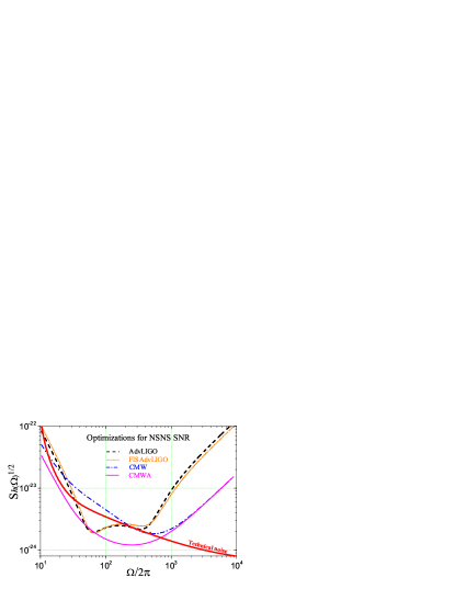
Figure 2: Quantum-noise spectrums of different schemes with optimized parameters for detecting gravitational waves from NSNS binaries. The optimal values for the parameters are listed in Table. 2.

The corresponding quantum-noise spectrums of different schemes optimized for detecting gravitational waves from NSNS binaries are shown in Fig. 2. The FISAdvLIGO, FISAdvLIGO and CMW schemes almost have the identical integrated sensitivity and CMWA scheme shows moderate $20\%$ improvement in SNR. This is attributable to the fact that the signal spectrum of NSNS binaries has a $f^{-7/3}$ dependence and low-frequency sensitivity is very crucial. However, due to low-frequency technical noise, advantages of the CMWA scheme are at most limited in the case for detecting low-frequency sources.

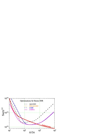
Figure 3: Quantum-noise spectrums of different schemes which are optimized for detecting gravitational waves from Bursts. The optimal values for the parameters are listed in Table. 2.

The case for detecting gravitational waves from Bursts is shown in Fig. 3. All other three schemes have a significant $50\%$ improvement in terms of SNR over AdvLIGO. The sensitivities of the optimal FISAdvLIGO, CMW and CMWA at high frequencies almost overlap each other. In addition, detuned phase $\phi_{\rm SR}$ of the signal recycling cavity of those three are nearly equal to $\pi/2$, which significantly increases the effective detection bandwidth of the gravitational-wave detectors and is the same as the resonant-sideband extraction scheme. This is because a broadband sensitivity is preferable in the case of Bursts which have a logarithmic flat spectrum.

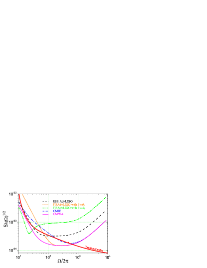
Figure 4: Quantum-noise spectrums of different schemes using the same parameters as the optimal CMWA to show how different parameters affect sensitivity of the CMWA scheme.

To show explicitly how different parameters affect sensitivity of the CMWA scheme, we present quantum-noise spectrums of different schemes using the same parameters as the optimal CMWA in Fig. 4. In the case of AdvLIGO, we obtain a resonant-sideband extraction (RSE) configuration with $\phi_{\rm SR}\approx\pi/2$. The quantum noise of FISAdvLIGO with squeezing angle $\theta=\theta_{s}$ is lower at high frequencies but higher at low frequencies than the RSE AdvLIGO. FISAdvLIGO with $\theta=\theta_{p}$ behaves in the opposite way with significant increase of sensitivity at low frequencies but worse at high frequencies. The CMW scheme with double squeezed-input, just as expected, can improve the sensitivity at both high and low frequencies but performs not so well at the intermediate frequencies. The CMWA scheme performs very nice over the whole observational band compared with others and it would be more attractive if the technical noise of the AdvLIGO design can be further decreased.

IV Conclusion

We have proposed and analyzed the double squeezed-input CMWA scheme as an option for increasing sensitivity of future advanced gravitational-wave detectors. Given an achievable optical loss of the filter cavity and 10dB squeezing, this CMWA configuration shows a noticeable reduction in quantum noise at both high and low frequencies compared with other schemes. Since the length of the filter cavity considered here is around $30$ m, with the developments of low-loss coating and better squeezing-state sources, it could be a promising and relatively simple add-on to AdvLIGO without a need for dramatically modifying the existing topology.

ACKNOWLEDGEMENTS

We thank S.L. Danilishin for invaluable discussions. F. Ya. Khalili’s research has been supported by NSF and Caltech Grant No. PHY-0651036. H. Miao’s research was supported by the Australian Research Council and the Department of Education, Science and Training. Y. Chen’s research was supported by the Alexander von Humboldt Foundation’s Sofja Kovalevskaja Programme, NSF grants PHY-0653653 and PHY-0601459, as well as the David and Barbara Groce startup fund at Caltech. H. Miao would like to thank D. G. Blair, J. Li and C. Zhao for their keen supports of his visiting to the Max Planck Institute and Caltech.

References

- (1) T. Corbitt, N. Mavalvala, and S. Whitcomb, Phys. Rev. D 70, 022002 (2004).
- (2) F. Ya. Khalili, Phys. Rev. D 77, 062003 (2008).
- (3) The LIGO project Web site, http://www.ligo.caltech.edu.
- (4) The VIRGO project Web site, http://www.virgo.infn.it/.
- (5) The GEO600 project Web site, http://geo600.aei.mpg.de.
- (6) The TAMA project Web site, http://tamago.mtk.nao.ac.jp.
- (7) The AdvLIGO project Web site, http://www.ligo.caltech.edu/advLIGO.
- (8) K. S. Thorne, in Three Hundred Years of Gravitation, edited by S. W. Hawking and W. Israel, Cambridg University Press, Cambridge, England, (1987).
- (9) V. B. Braginsky, Sov. Phys. JETP 26, 831 (1968).
- (10) V. B. Braginsky and F. Ya. Khalili, in Quantum Measurement, edited by K. S. Thorne Cambridge University Press, Cambridge, England, (1992).
- (11) F. Ya. Khalili and Yu. Levin, Phys. Rev. D 54, 004735 (1996).
- (12) V. B. Braginsky, M. L. Gorodetsky, F. Ya. Khalili, and K. S. Thorne, Phys. Rev. D 61, 044002 (2000).
- (13) P. Purdue, Phys. Rev. D 66, 022001 (2002).
- (14) P. Purdue and Y. Chen, Phys. Rev. D 66, 122004 (2002).
- (15) Y. Chen, Phys. Rev. D 67, 122004 (2003).
- (16) S. L. Danilishin, Phys. Rev. D 69, 102003 (2004).
- (17) V. B. Braginsky, and F. Ya. Khalili, Phys. Lett. A 257, 241 (1999).
- (18) F. Ya. Khalili, Phys. Lett. A 288, 251 (2001).
- (19) A. Buonanno and Y. Chen, Phys. Rev. D 64, 042006 (2001).
- (20) A. Buonanno and Y. Chen, Phys. Rev. D 65, 042001 (2002).
- (21) A. Buonanno and Y. Chen, Phys. Rev. D 67, 062002 (2003).
- (22) E. G. Unruh, in Quantum Optics, Experimental Gravitation, and Measurement Theory, edited by P.Meystre and M.O.Scully, page 647, 1982.
- (23) F. Ya. Khalili, Dokl. Akad. Nauk SSSR 294, 602 (1987) (see also Braginsky2 , Chapter 8).
- (24) M. T. Jaekel and S. Reynaud, Europhysics Letters 13, 301 (1990).
- (25) A. F. Pace, M. J. Collett and D. F. Walls, Phys. Rev. A 47, 3173 (1993).
- (26) S. P. Vyatchanin and E. A. Zubova, Phys. Lett. A 203, 269 (1995).
- (27) H. J. Kimble, Y. Levin, A. B. Matsko, K. S. Thorne, and S. P. Vyatchanin, Phys. Rev. D 65, 022002 (2001) and reference therein.
- (28) A. Buonanno and Y. Chen, Phys. Rev. D 69, 102004 (2004).
- (29) O. Arcizet, T. Briant, A. Heidmann and M. Pinard, Phys. Rev. A 73, 033819 (2006).
- (30) F. Ya. Khalili, Phys. Rev. D 76, 102002 (2007).
- (31) K. McKenzie, N. Grosse, W. P. Bowen, S. E. Whitcomb, M. B. Gray, D. E. McClelland, and P. K. Lam, Phys. Rev. Lett. 93, 161105 (2004).
- (32) H. Vahlbruch, S. Chelkowski, B. Hage, A. Franzen, K. Danzmann, and R. Schnabel, Phys. Rev. Lett. 97, 011101 (2006).
- (33) F. Ya. Khalili, V. I. Lazebny and S. P. Vyatchanin, Phys. Rev. D 73, 062002 (2006).
- (34) L. Yungelson and K. Postnov, Living Rev. Relativity 9, 6 (2006).
- (35) I. S. Kondrashov, D. A. Simakov, F. Ya. Khalili and S. L. Danilishin, Phys. Rev. D 78, 062004 (2008).
- (36) B. Abbott et al. (LIGO Scientific Collaboration), Phys. Rev. D 69, 102001 (2004); Phys. Rev. D 72, 122004 (2005); Classical Quantum Gravity 24, 5343 (2007).
- (37) http://ilog.ligo-wa.caltech.edu:7285/advligo/Bench.