Calculation of Drag and Superfluid Velocity from the Microscopic Parameters and Excitation Energies of a Two-Component Bose-Einstein Condensate on an Optical Lattice

Abstract

We investigate a model of a two-component Bose-Einstein condensate residing on an optical lattice. Within a Bogolioubov-approach at the mean-field level, we derive exact analytical expressions for the excitation spectrum of the two-component condensate when taking into account hopping and interactions between arbitrary sites. Our results thus constitute a basis for works that seek to clarify the effects of higher-order interactions in the system. We investigate the excitation spectrum and the two branches of superfluid velocity in more detail for two limiting cases of particular relevance. Moreover, we relate the hopping and interaction parameters in the effective Bose-Hubbard model to microscopic parameters in the system, such as the laserlight wavelength and atomic masses of the components in the condensate. These results are then used to calculate analytically and numerically the drag coefficient between the components of the condensate. We find that the drag is most effective close to the symmetric case of equal masses between the components, regardless of the strength of the intercomponent interaction and the lattice well depth.

I Introduction

The emergence of laser cooling techniques and their applications to realizing the phenomenon of Bose-Einstein condensation (BEC) in the laboratory, has paved the way for a study of the rich physics present when atoms condense at ultralow temperatures on an optical lattice dalfovo_rmp_99 ; leggett_rmp_01 ; morsch_rmp_06 . The BEC itself is a coherent matter wave, and has attracted much attention both theoretically and experimentally over the past decade. One of the remarkable features of a BEC residing on an optical lattice is the extent to which physical quantities such as tunnel coupling and on-site interaction may be controlled experimentally simply by adjusting the lattice parameters. This is done by controlling the interference pattern of the lasers setting up the optical lattice. For instance, by causing the depth of the lattice potential to increase, when would expect a resultant decrease of the hopping amplitudes and an increase of the on-site interaction. The possibility to alter the lattice parameters directly during the experiment, and thus influencing the physics, is clearly intriguing. Moreover, experiments carried out on such systems are extremely well controlled since there is no disorder present. Since the atoms reside on an enginereed lattice, it is possible to investigate the physics by means of standard theories in condensed matter physics, such as the Bose-Hubbard model jaksch_prl_98 . As pointed out in Ref. morsch_rmp_06 , BECs residing on optical lattices have several advantages compared to ultracold atoms in a non-condensed phase. The main point is that the temperatures and densities for ultracold atoms and BECs both differ by three to four orders of magnitude. One consequence of the much higher particle densities for BECs is that atomic interactions become crucial with regard to the physics.

By allowing for more than one component of bosonic atoms on an optical lattice, one opens up an exciting avenue of physics to explore mazzarella_pra_06 ; chen_pra_03 ; fil_pra_05 ; kaurov_prl_05 ; dahl_prb_08 ; dahl_prl_09 . The physical realization of such a multicomponent BEC includes condensates with spin degrees of freedom (spinor condensates), two or more hyperfine states of the same atomic species that condense simultaneously, or simply two distinct atomic species. The two-component condensate has been shown to be a more rich environment to explore than a single-component BEC due to the possibility of an “entrainment” coupling between the condensate components, see Ref. dahl_prb_08, ; dahl_prl_09, and references therein. Such a system may be studied at a mean-field level by employing a Bogolioubov-approach, which may provide information about both the transition from a superfluid to Mott insulating state and also the quasiparticle excitation energies which arise from the condensate. By means of the Landau criterion, it is also possible to obtain information about the superfluid velocity of the condensate from the excitation spectrum.

Figure 1: (Color online) An optical lattice setup by counter-propagating lasers serves as a potential landscape for two atomic species, denoted by the red (dark) and green (light) spheres. Each species of atoms may hop from site to site and also interact with both inter- and intraspecies atoms.

Very recently, the excitation spectrum for a two-component Bose-Einstein condensate was obtained for a limiting case in Ref. liu_pra_07 . In that work, the author presented a correction to erroneous results previously reported in the literature gu_pla_05 . The calculations were performed under the standard assumptions of nearest-neighbor hopping and on-site interactions only. It would clearly be of interest extend calculations beyond these approximations, in order to investigate how the excitation spectrum is affected by taking into account longer-range hopping and longer-range interactions. One of the purposes of the present paper is to extend the calculations of Ref. liu_pra_07, in this direction.

Another goal in this paper is to address the effect of drag between the atomic components in a two-component Bose-Einstein condensate residing on an optical lattice. Such a drag effect points to a mutual transfer of motion between the components, and was first investigated in ³He-⁴He superfluid mixtures by Andreev and Bashkin andreev_bashkin . In Ref. fil_pra_05 , the drag effect for a two-component Bose gas was explored in the continuum limit. We will here derive an analytical expression for the intercomponent drag $\rho_{d}$ in a two-component Bose-Einstein condensate residing on an optical lattice, and relating it directly to the microscopic parameters in the system which are possible to tune experimentally.

We organize this paper as follows. In Sec. II, we establish the theoretical framework to be used in deriving our main results. In Sec. III, we provide an analytical solution for the excitation spectrum of a two-component Bose-Einstein condensate for arbitrary hopping and interaction between sites (Sec. III.1) and investigate the superfluid velocity and phase-separation condition in more detail for two limiting cases in Sec. III.2 and III.3. Also, we present a correction to the condition for phase-stability of the two components, which determines whether the species are spatially miscible or not. In Sec. III.4, we first relate analytically the parameters in the two-component Bose-Hubbard model directly to the fundamental physical quantities such as mass and trapping potential. Then, we combine these results with the expressions for the excitation energies in Sec. III.2 and obtain an analytical equation for the drag coefficient in the system. The drag coefficient is then studied as a function of the microscopic parameters. Finally, we give concluding remarks in Sec. IV. The system under consideration is shown schematically in Fig. 1.

II Theory

The starting point for our calculations is a microscopic Hamiltonian $\hat{H}$ for an ensemble of bosonic atoms that are confined by a slowly varying external harmonic trapping potential $V_{\text{T},\alpha}(\boldsymbol{r})$ and subject to an additional optical lattice potential $V_{0}(\boldsymbol{r})$. In terms of boson field operators $\psi_{\alpha}(\boldsymbol{r})$, where $\alpha$ denotes the boson-component, $\hat{H}$ may be written as $(\hbar=1)$

$$\hat{H}=\sum_{\alpha}\int\text{d}\boldsymbol{r}\psi_{\alpha}^{\dagger}(\boldsymbol{r})\Big{[}-\frac{\nabla^{2}}{2m_{\alpha}}-\mu_{\alpha}+V_{0}(\boldsymbol{r})+V_{\text{T},\alpha}(\boldsymbol{r})\Big{]}$$

$$\times\psi_{\alpha}(\boldsymbol{r})+\frac{1}{2}\sum_{\alpha\beta}\int\text{d}\boldsymbol{r}\psi^{\dagger}_{\alpha}(\boldsymbol{r})\psi^{\dagger}_{\beta}(\boldsymbol{r})\gamma_{\alpha\beta}\psi_{\beta}(\boldsymbol{r})\psi_{\alpha}(\boldsymbol{r}),$$ (1)

where $\gamma_{\alpha\beta}$ denotes the onsite-interaction for both boson species, $m_{\alpha}$ is the mass of boson species $\alpha$, and $\mu_{\alpha}$ is its chemical potential. Specifically, we have fil_pra_05

$$\gamma_{\alpha\beta}=\left\{\begin{array}[]{ll}4\pi a_{\alpha}/m_{\alpha}&\textrm{if $\alpha=\beta$}\\ 2\pi(m_{A}+m_{B})a_{AB}/m_{A}m_{B}&\textrm{if $\alpha\neq\beta$}\end{array}\right.$$

Here, $a_{\alpha},a_{AB}$ are intraspecies and interspecies $s$-wave scattering lengths. The interaction strength is assumed to be repulsive and, in general, different for each of the boson components: $\{a_{\alpha},a_{AB}\}>0$. To obtain a second-quantized Hamiltonian in a lattice-formulation, we assume that the field operators $\psi_{\alpha}(\boldsymbol{r})$ may be expanded in a Wannier function basis set. The physical motivation for this is that the bosons are assumed to spend most of their time in the minima of the optical lattice potential, with occasional tunneling from one site to another. In this case, a set of localized Wannier functions where only the lowest lying excitation level is taken into account is expected to be a reasonable choice of basis. We consider here a two-dimensional model, such that $\psi_{\alpha}(\boldsymbol{r})=\sum_{i}b_{i\alpha}w_{\alpha}(x-x_{i})w_{\alpha}(y-y_{i})$. Here, $b_{i\alpha}$ are boson annihilation operators for species $\alpha$ on the lattice point $i$, while $W_{\alpha}(\boldsymbol{r}-\boldsymbol{r}_{i})=w_{\alpha}(x-x_{i})w_{\alpha}(y-y_{i})$ are single-particle Wannier states for boson species $\alpha$ centred around lattice point $i$ at $(x_{i},y_{i})$. Inserting this expansion into Eq. (II) yields an effective Bose-Hubbard like model, defined by the Hamiltonian

$$\hat{H} =-\sum_{\alpha}\sum_{i\neq j}t_{ij\alpha}b_{i\alpha}^{\dagger}b_{j\alpha}+\sum_{i\alpha}\varepsilon_{i\alpha}b_{i\alpha}^{\dagger}b_{i\alpha}$$

$$+\frac{1}{2}\sum_{ijkl}\sum_{\alpha\beta}U_{ijkl\alpha\beta}b_{i\alpha}^{\dagger}b_{j\beta}^{\dagger}b_{k\beta}b_{l\alpha}.$$ (2)

The parameters of this model are expressed as

$$t_{ij\alpha} =-\int\text{d}\boldsymbol{r}W_{\alpha}^{*}(\boldsymbol{r}-\boldsymbol{r}_{i})\Big{[}-\frac{\nabla^{2}}{2m_{\alpha}}+V_{0}(\boldsymbol{r})$$

$$\hskip 86.72377pt+V_{\text{T},\alpha}(\boldsymbol{r})\Big{]}W_{\alpha}(\boldsymbol{r}-\boldsymbol{r}_{j}),$$

$$\varepsilon_{i\alpha} =\int\text{d}\boldsymbol{r}W_{\alpha}^{*}(\boldsymbol{r}-\boldsymbol{r}_{i})\Big{[}-\frac{\nabla^{2}}{2m_{\alpha}}-\mu_{\alpha}+V_{0}(\boldsymbol{r})$$

$$\hskip 86.72377pt+V_{\text{T},\alpha}(\boldsymbol{r})\Big{]}W_{\alpha}(\boldsymbol{r}-\boldsymbol{r}_{i}),$$

$$U_{ijkl\alpha\beta} =\gamma_{\alpha\beta}\int\text{d}\boldsymbol{r}W_{\alpha}^{*}(\boldsymbol{r}-\boldsymbol{r}_{i})W_{\beta}^{*}(\boldsymbol{r}-\boldsymbol{r}_{j})$$

$$\hskip 39.74872pt\times W_{\beta}(\boldsymbol{r}-\boldsymbol{r}_{k})W_{\alpha}(\boldsymbol{r}-\boldsymbol{r}_{l}).$$ (3)

So far, we have made no approximations apart from the assumed field expansion. The integrals given above may be evaluated analytically by specifying the explicit form of $W_{\alpha}(\boldsymbol{r})$. Let us consider the following generic form for the trap and laser potential:

$$V_{\text{T},\alpha}(\boldsymbol{r}) =\frac{m_{\alpha}}{2}(\omega_{x}^{2}x^{2}+\omega_{y}^{2}y^{2}+\omega_{z}z^{2}),$$

$$V_{0}(\boldsymbol{r}) =V_{x}\sin^{2}(k_{x}x)+V_{y}\sin^{2}(k_{y}y)+V_{z}\sin^{2}(k_{z}z).$$ (4)

Here, $\omega_{j}$ is the frequency of harmonic trapping potential associated with the $j$-direction while the wave vector $k_{j}$ for the optical lattice is related to the wavelength $\lambda$ of the laser light as $k_{j}=2\pi/\lambda_{j}$, such that the lattice period becomes $a_{j}=\lambda_{j}/2$, $j\in\{x,y,z\}$. In the harmonic approximation jaksch_prl_98 ; giampaolo_pra_04 , where the bosons have a small probability of being located far from each lattice site and higher energy states in each lattice potential may be neglected, the exact Wannier functions can be replaced with their harmonic-oscillator approximation to a satisfactory degree. Then, one may write

$$w_{\alpha}(x-x_{i}) =\Big{(}\frac{m_{\alpha}\tilde{\omega}_{x,\alpha}}{\pi}\Big{)}^{1/4}\mathrm{e}^{-m_{\alpha}(x-x_{i})^{2}/2},$$

$$\tilde{\omega}_{x,\alpha} =\sqrt{\omega_{x}^{2}+2V_{x}k_{x}^{2}/m_{\alpha}}.$$ (5)

and similarly for $w_{\alpha}(y-y_{i})$ and $w_{\alpha}(z-z_{i})$. Since the Wannier functions are known, one may derive analytical expressions that relate the parameters in Eq. (II) to the microscopic parameters in the system. For the hopping term $t_{ij,\alpha}$, previous works have neglected the influence of the trapping potential on this parameter by demanding that $V_{\text{T},\alpha}(\boldsymbol{r})$ varies much more slowly than $V_{0}(\boldsymbol{r})$. In this work, we derive a more general expression for both the hopping parameter and the interaction term by generalizing previous results to the two-component case and also by including the effect of the trapping potential. This is done towards the end of Sec. III

III Results

We now proceed to derive an analytical expression for the excitation energies of the elementary quasiparticles of the condensate. The standard approximation consists of only considering nearest-neighbor hopping and on-site interactions. To begin with, we include all orders of hopping and interactions without any site-limitation. We then explicitly consider two cases of particular relevance. Finally, we relate the microscopic parameters of the system to the hopping and interaction term in the effective Bose-Hubbard Hamiltonian.

III.1 General solution

By introducing a mean-field decomposition of the interaction terms allows us to consider the case where a macroscopic number of particles have condensed into the zero-momentum state. Let us define the Fourier-transformed boson operators

$$b_{i\alpha}=\frac{1}{\sqrt{N_{s}}}\sum_{\boldsymbol{k}}b_{{\boldsymbol{k}}\alpha}\mathrm{e}^{-i{\boldsymbol{k}}\mathbf{r}_{i}},$$ (6)

which inserted into Eq. (II) may be written as

$$H =\sum_{{\boldsymbol{k}}\alpha}(\varepsilon_{{\boldsymbol{k}},\alpha}+T_{\alpha})b_{{\boldsymbol{k}}\alpha}^{\dagger}b_{{\boldsymbol{k}}\alpha}+\frac{1}{N_{s}}\sum_{\{{\boldsymbol{k}}_{i}\}}\Big{[}\sum_{\alpha}\frac{1}{2}\tilde{U}_{\alpha}({\boldsymbol{k}}_{2},{\boldsymbol{k}}_{3},{\boldsymbol{k}}_{4})$$

$$\times b_{{\boldsymbol{k}}_{1}\alpha}^{\dagger}b_{{\boldsymbol{k}}_{2}\alpha}^{\dagger}b_{{\boldsymbol{k}}_{3}\alpha}b_{{\boldsymbol{k}}_{4}\alpha}\delta_{{\boldsymbol{k}}_{1}+{\boldsymbol{k}}_{2},{\boldsymbol{k}}_{3}+{\boldsymbol{k}}_{4}}+\tilde{U}_{AB}({\boldsymbol{k}}_{1},{\boldsymbol{k}}_{2},{\boldsymbol{k}}_{3},{\boldsymbol{k}}_{4})$$

$$\times b_{{\boldsymbol{k}}_{1}A}^{\dagger}b_{{\boldsymbol{k}}_{2}A}b_{{\boldsymbol{k}}_{3}B}^{\dagger}b_{{\boldsymbol{k}}_{4}B}\delta_{{\boldsymbol{k}}_{1}+{\boldsymbol{k}}_{3},{\boldsymbol{k}}_{2}+{\boldsymbol{k}}_{4}}\Big{]},$$ (7)

where we have defined the generalized intraspecies potential

$$\tilde{U}_{\alpha}({\boldsymbol{k}}_{2},{\boldsymbol{k}}_{3},{\boldsymbol{k}}_{4}) =U_{\alpha}(0,0,0)+\sum_{\{\boldsymbol{\delta}_{i}\}}U_{\alpha}(\boldsymbol{\delta}_{1},\boldsymbol{\delta}_{2},\boldsymbol{\delta}_{3})$$

$$\times\mathrm{e}^{\mathrm{i}({\boldsymbol{k}}_{2}\cdot\boldsymbol{\delta}_{1}-{\boldsymbol{k}}_{3}\cdot\boldsymbol{\delta}_{2}-{\boldsymbol{k}}_{4}\cdot\boldsymbol{\delta}_{3})},$$ (8)

and the interspecies potential

$$\tilde{U}_{AB} ({\boldsymbol{k}}_{1},{\boldsymbol{k}}_{2},{\boldsymbol{k}}_{3},{\boldsymbol{k}}_{4})=U_{AB}(0,0,0)+\sum_{\{\boldsymbol{\delta}_{i}\}}U_{AB}(\boldsymbol{\delta}_{1},\boldsymbol{\delta}_{2},\boldsymbol{\delta}_{3})$$

$$\times(\mathrm{e}^{\mathrm{i}({\boldsymbol{k}}_{1}\cdot\boldsymbol{\delta}_{1}-{\boldsymbol{k}}_{2}\cdot\boldsymbol{\delta}_{2}-{\boldsymbol{k}}_{4}\cdot\boldsymbol{\delta}_{3})}+\mathrm{e}^{\mathrm{i}({\boldsymbol{k}}_{3}\cdot\boldsymbol{\delta}_{1}-{\boldsymbol{k}}_{4}\cdot\boldsymbol{\delta}_{2}-{\boldsymbol{k}}_{2}\cdot\boldsymbol{\delta}_{3})}).$$ (9)

Above, the quantities $U_{\alpha}(\boldsymbol{\delta}_{1},\boldsymbol{\delta}_{2},\boldsymbol{\delta}_{3})$ and $U_{AB}(\boldsymbol{\delta}_{1},\boldsymbol{\delta}_{2},\boldsymbol{\delta}_{3})$ denote the interaction strengths and their dependence on the site distance between the particles involved in the scattering process, while $N_{s}$ denotes the number of lattice sites. Also, we have assumed that the energy off-set at each lattice site is simply a constant $\varepsilon_{i\alpha}=T_{\alpha}$. The interactions are related to the scattering potential $U_{ijkl\alpha\beta}$ as follows

$$U_{\alpha}(\boldsymbol{\delta}_{1},\boldsymbol{\delta}_{2},\boldsymbol{\delta}_{3})=U_{i,i+\boldsymbol{\delta}_{1},i+\boldsymbol{\delta}_{2},i+\boldsymbol{\delta}_{3},\alpha\alpha},$$

$$U_{AB}(\boldsymbol{\delta}_{1},\boldsymbol{\delta}_{2},\boldsymbol{\delta}_{3})=U_{i,i+\boldsymbol{\delta}_{1},i+\boldsymbol{\delta}_{2},i+\boldsymbol{\delta}_{3},AB},$$

and are thus assumed to be independent on at which particular lattice site $i$ the scattering takes place, as is reasonable. The kinetic energy term is given by

$$\varepsilon_{{\boldsymbol{k}},\alpha}=-\sum_{\boldsymbol{\delta}}t_{\alpha}(\boldsymbol{\delta})\mathrm{e}^{-\mathrm{i}{\boldsymbol{k}}\cdot\boldsymbol{\delta}},$$ (11)

where the summation over $\boldsymbol{\delta}$ is to be taken over all neighbor sites. In Eqs. (III.1) and (III.1), the summation over $\{\boldsymbol{\delta}_{i}\}=(\boldsymbol{\delta}_{1},\boldsymbol{\delta}_{2},\boldsymbol{\delta}_{3})$ is to be taken over all possible combinations of on-site and off-site lattice points except for pure on-site scattering $\{\boldsymbol{\delta}_{i}\}=\{\boldsymbol{0}\}$. In this way, the first term in Eqs. (III.1) and (III.1) represents the on-site interaction while the second term incorporates scattering involving multiple sites.

Since we are considering the condensed phase, we may write

$$b_{0\alpha}b_{0\alpha}^{\dagger}=b_{0\alpha}^{\dagger}b_{0\alpha}+1\simeq N_{0\alpha}\gg 1,$$

$$N_{0\alpha}=N_{\alpha}-\sum_{{\boldsymbol{k}}}^{\prime}b_{{\boldsymbol{k}}\alpha}^{\dagger}b_{{\boldsymbol{k}}\alpha},$$ (12)

where the ^′ superscript over the sum denotes summation over all modes except ${\boldsymbol{k}}=0$. Physically, we are stating that the number of atoms in the zero-mode state ${\boldsymbol{k}}=0$ dominates the contribution to the total number of atoms for all ${\boldsymbol{k}}$-modes. The biquadratic terms may be reduced to bilinear form by retaining only the interaction between the ${\boldsymbol{k}}=0$ modes and other ${\boldsymbol{k}}\neq 0$ modes. Since the number of atoms $N_{0\alpha}$ in the ${\boldsymbol{k}}=0$ mode for atom species $\alpha$ is assumed to satisfy Eq. (III.1), we may replace $b_{0\alpha}=b_{0\alpha}^{\dagger}=\sqrt{N_{0\alpha}}$.

Next, we explicitly take into account the $\delta$-function constraints on the particle momenta in Eq. (III.1), which allows us to reduce the Hamiltonian to a sum over the atom species $\alpha$ and a single sum over momentum ${\boldsymbol{k}}$. In this way, one obtains

$$H=H_{0}+\sum_{\boldsymbol{k}}^{\prime}\Big{[}H_{AB}+\sum_{\alpha}H_{\alpha}\Big{]},$$ (13)

where we have defined

$$H_{0} =\sum_{\alpha}\Big{[}N_{\alpha}(T_{\alpha}+\varepsilon_{0,\alpha})+\frac{N_{\alpha}^{2}}{2N_{s}}\tilde{U}_{\alpha}(0,0,0)\Big{]}$$

$$+\frac{N_{A}N_{B}}{N_{s}}\tilde{U}_{AB}(0,0,0,0)$$ (14)

and the interaction terms

$$H_{\alpha} =\epsilon_{\boldsymbol{k}}^{\alpha}+(n_{\alpha}/2)[\tilde{U}_{\alpha}({\boldsymbol{k}},0,{\boldsymbol{k}})+\tilde{U}_{\alpha}(0,{\boldsymbol{k}},0)+\tilde{U}_{\alpha}(0,0,{\boldsymbol{k}})+\tilde{U}_{\alpha}({\boldsymbol{k}},{\boldsymbol{k}},0)-2\tilde{U}_{\alpha}(0,0,0)]b_{{\boldsymbol{k}}\alpha}^{\dagger}b_{{\boldsymbol{k}}\alpha}$$

$$+(n_{\alpha}/2)[\tilde{U}_{\alpha}(-{\boldsymbol{k}},0,0)b_{{\boldsymbol{k}}\alpha}^{\dagger}b_{-{\boldsymbol{k}}\alpha}^{\dagger}+\tilde{U}_{\alpha}(0,{\boldsymbol{k}},-{\boldsymbol{k}})b_{{\boldsymbol{k}}\alpha}b_{-{\boldsymbol{k}}\alpha}]$$ (15)

$$H_{AB} =[\tilde{U}_{AB}({\boldsymbol{k}},0,0,{\boldsymbol{k}})b_{{\boldsymbol{k}}A}^{\dagger}b_{{\boldsymbol{k}}B}+\tilde{U}_{AB}(0,{\boldsymbol{k}},{\boldsymbol{k}},0)b_{{\boldsymbol{k}}A}b_{{\boldsymbol{k}}B}^{\dagger}+\tilde{U}_{AB}({\boldsymbol{k}},0,-{\boldsymbol{k}},0)b_{{\boldsymbol{k}}A}^{\dagger}b_{-{\boldsymbol{k}}B}^{\dagger}+\tilde{U}_{AB}(0,{\boldsymbol{k}},-{\boldsymbol{k}},0)b_{{\boldsymbol{k}}A}b_{-{\boldsymbol{k}}B}]$$

$$\times\sqrt{n_{A}n_{B}}+n_{A}[\tilde{U}_{AB}(0,0,{\boldsymbol{k}},{\boldsymbol{k}})-\tilde{U}_{AB}(0,0,0,0)]b_{{\boldsymbol{k}}B}^{\dagger}b_{{\boldsymbol{k}}B}+n_{B}[\tilde{U}_{AB}({\boldsymbol{k}},{\boldsymbol{k}},0,0)-\tilde{U}_{AB}(0,0,0,0)]b_{{\boldsymbol{k}}A}^{\dagger}b_{{\boldsymbol{k}}A},$$ (16)

where $\epsilon_{\boldsymbol{k}}^{\alpha}=\varepsilon_{{\boldsymbol{k}}\alpha}+\sum_{\boldsymbol{\delta}}t_{\alpha}(\boldsymbol{\delta})$. The above equation describes the Hamiltonian of a two-component Bose-Einstein condensate residing on an optical lattice with a drag between the atomic species. By diagonalizing Eq. (13), we obtain the quasiparticle spectrum which allows for a further study of the different phases that may be expected for the condensate and also how the superfluid velocity depends on the interaction parameters. Using the basis

$$\phi_{\boldsymbol{k}}=[b_{{\boldsymbol{k}}A},b_{-{\boldsymbol{k}}A},b_{{\boldsymbol{k}}B},b_{-{\boldsymbol{k}}B},b^{\dagger}_{{\boldsymbol{k}}A},b^{\dagger}_{-{\boldsymbol{k}}A},b^{\dagger}_{{\boldsymbol{k}}B},b^{\dagger}_{-{\boldsymbol{k}}B}]^{\text{T}},$$ (17)

the Hamiltonian can now be written in compact matrix form:

$$H=H_{0}+\frac{1}{4}\sum_{\boldsymbol{k}}^{\prime}\phi_{\boldsymbol{k}}^{\dagger}\check{\mathcal{M}}_{\boldsymbol{k}}\phi_{\boldsymbol{k}},$$ (18)

where the matrix $\check{\mathcal{M}}_{\boldsymbol{k}}$ reads

$$\check{\mathcal{M}}_{\boldsymbol{k}} =\begin{pmatrix}\hat{M}_{1}({\boldsymbol{k}})&\hat{M}_{2}({\boldsymbol{k}})\\ \hat{M}_{2}({\boldsymbol{k}})^{*}&\hat{M}_{1}({\boldsymbol{k}})^{*}\\ \end{pmatrix},$$ (19)

upon defining the auxiliary matrices

$$\hat{M}_{1}({\boldsymbol{k}}) =\begin{pmatrix}E_{A}({\boldsymbol{k}})&0&V_{1}({\boldsymbol{k}})&0\\ 0&E_{A}(-{\boldsymbol{k}})&0&V_{1}(-{\boldsymbol{k}})\\ V_{1}^{*}({\boldsymbol{k}})&0&E_{B}({\boldsymbol{k}})&0\\ 0&V_{1}^{*}(-{\boldsymbol{k}})&0&E_{B}(-{\boldsymbol{k}})\\ \end{pmatrix},$$

$$\hat{M}_{2}({\boldsymbol{k}}) =\begin{pmatrix}0&U_{A}({\boldsymbol{k}})&0&V_{2}^{*}({\boldsymbol{k}})\\ U_{A}({\boldsymbol{k}})&0&V_{2}^{*}(-{\boldsymbol{k}})&0\\ 0&V_{2}^{*}(-{\boldsymbol{k}})&0&U_{B}({\boldsymbol{k}})\\ V_{2}^{*}({\boldsymbol{k}})&0&U_{B}({\boldsymbol{k}})&0\\ \end{pmatrix}.$$ (20)

We have introduced the following notation:

$$E_{A}({\boldsymbol{k}})=\epsilon_{\boldsymbol{k}}^{A} +\frac{n_{A}}{2}[\tilde{U}_{A}({\boldsymbol{k}},0,{\boldsymbol{k}})+\tilde{U}_{A}(0,{\boldsymbol{k}},0)+\tilde{U}_{A}(0,0,{\boldsymbol{k}})+\tilde{U}_{A}({\boldsymbol{k}},{\boldsymbol{k}},0)-2\tilde{U}_{A}(0,0,0)]$$

$$+n_{B}[\tilde{U}_{AB}({\boldsymbol{k}},{\boldsymbol{k}},0,0)-\tilde{U}_{AB}(0,0,0,0)],$$

$$E_{B}({\boldsymbol{k}})=\epsilon_{\boldsymbol{k}}^{B} +\frac{n_{B}}{2}[\tilde{U}_{B}({\boldsymbol{k}},0,{\boldsymbol{k}})+\tilde{U}_{B}(0,{\boldsymbol{k}},0)+\tilde{U}_{B}(0,0,{\boldsymbol{k}})+\tilde{U}_{B}({\boldsymbol{k}},{\boldsymbol{k}},0)-2\tilde{U}_{B}(0,0,0)]$$

$$+n_{A}[\tilde{U}_{AB}(0,0,{\boldsymbol{k}},{\boldsymbol{k}})-\tilde{U}_{AB}(0,0,0,0)],$$

$$U_{j}({\boldsymbol{k}}) =n_{j}\tilde{U}_{j}(-{\boldsymbol{k}},0,0)\text{ with }j=A,B,\;V_{1}({\boldsymbol{k}})=\sqrt{n_{A}n_{B}}\tilde{U}_{AB}({\boldsymbol{k}},0,0,{\boldsymbol{k}}),\;V_{2}({\boldsymbol{k}})=\sqrt{n_{A}n_{B}}\tilde{U}_{AB}(0,{\boldsymbol{k}},-{\boldsymbol{k}},0).$$ (21)

In order to obtain Eqs. (19) and (III.1), we made use of the fact that the matrix $\check{\mathcal{M}}_{\boldsymbol{k}}\check{\sigma}_{3}$ must be Hermitian, since the eigenvalues have to be real (see discussion below). Our ultimate goal is to obtain a Hamiltonian that may be written as

$$H=\tilde{H}_{0}+\frac{1}{4}\sum_{\boldsymbol{k}}^{\prime}\Phi_{\boldsymbol{k}}^{\dagger}\check{\mathcal{D}}_{\boldsymbol{k}}\Phi_{\boldsymbol{k}},$$ (22)

where the matrix $\check{\mathcal{D}}_{\boldsymbol{k}}$ contains the excitation energies. Note that $\tilde{H}_{0}$ will in general be different from $H_{0}$. The new basis $\Phi_{\boldsymbol{k}}$ is related to the old one $\phi_{\boldsymbol{k}}$ through the diagonalization matrix $\check{T}_{\boldsymbol{k}}$, and also satsifies the correct boson commutation relation: $\Phi_{\boldsymbol{k}}=\check{T}_{\boldsymbol{k}}^{\dagger}\phi_{\boldsymbol{k}},\;\Phi_{\boldsymbol{k}}\Phi_{\boldsymbol{k}}^{\dagger}-(\Phi_{\boldsymbol{k}}^{\dagger}\Phi_{\boldsymbol{k}})^{\mathcal{T}}=\check{\sigma}_{3}.$ From the requirement that the new basis also consists of boson operators, one finds that the relation $\check{T}_{\boldsymbol{k}}^{\dagger}\check{\sigma}_{3}\check{T}_{\boldsymbol{k}}=\check{\sigma}_{3}$ must be satisfied. From this, one may infer that $(\check{\mathcal{M}}_{\boldsymbol{k}}\check{\sigma}_{3})=\check{T}_{\boldsymbol{k}}(\check{D}_{\boldsymbol{k}}\check{\sigma}_{3})\check{T}_{\boldsymbol{k}}^{-1},$ which means that $\check{T}_{\boldsymbol{k}}$ diagonalizes the matrix $(\check{\mathcal{M}}_{\boldsymbol{k}}\check{\sigma}_{3})$. The corresponding eigenvalues are contained in the matrix $\check{D}_{\boldsymbol{k}}\check{\sigma}_{3}$, and may be determined by considering $|\check{\mathcal{M}}_{\boldsymbol{k}}\check{\sigma}_{3}-\Lambda\check{1}|=0$. Evaluating the above determinant yields four distinct eigenvalues $\Lambda_{\boldsymbol{k}}=\pm\mathcal{E}_{{\boldsymbol{k}}\sigma}$, $\sigma=\pm 1$.

Before carrying out the diagonalization procedure, it is advantadgeous to make a simplifying observation: if the interaction potential satisfies

$$U_{\alpha}(\boldsymbol{\delta}_{1},\boldsymbol{\delta}_{2},\boldsymbol{\delta}_{3})=U_{\alpha}(-\boldsymbol{\delta}_{1},-\boldsymbol{\delta}_{2},-\boldsymbol{\delta}_{3}),$$ (23)

and similarly for $\alpha\to AB$, one may verify directly that $\{U_{A}({\boldsymbol{k}}),U_{B}({\boldsymbol{k}}),V_{1}({\boldsymbol{k}}),V_{2}({\boldsymbol{k}})\}$ in Eq. (III.1) are all even under inversion of momentum, i.e. ${\boldsymbol{k}}\to(-{\boldsymbol{k}})$. Physically, Eq. (23) expresses that the scattering potential for a set of lattice sites and the sites obtained upon a mirror transformation, as shown in Fig. 2, which is the case e.g. for a square lattice. In addition, one may verify that $\{U_{A}({\boldsymbol{k}}),U_{B}({\boldsymbol{k}}),V_{1}({\boldsymbol{k}}),V_{2}({\boldsymbol{k}})\}$ must all be real quantities for the same reason.

Thus, we are finally able to give an analytical expression for the excitation energies $\Lambda_{\boldsymbol{k}}$ for a two-component Bose-Einstein condensate with drag when taking into account arbitrary hopping and interaction between arbitrary sites. We find that

$$\mathcal{E}_{{\boldsymbol{k}}\sigma}=\frac{1}{2}\Big{[} 2[E_{B}^{2}({\boldsymbol{k}})+E_{A}^{2}({\boldsymbol{k}})]+4[V_{1}^{2}({\boldsymbol{k}})-V_{2}^{2}({\boldsymbol{k}})]-2[U_{A}^{2}({\boldsymbol{k}})+U_{B}^{2}({\boldsymbol{k}})]+2\sigma\sqrt{R({\boldsymbol{k}})}\Big{]}^{1/2},$$ (24)

where we have introduced

$$R({\boldsymbol{k}}) =8[V_{1}^{2}({\boldsymbol{k}})+V_{2}^{2}({\boldsymbol{k}})][U_{A}({\boldsymbol{k}})U_{B}({\boldsymbol{k}})+E_{A}({\boldsymbol{k}})E_{B}({\boldsymbol{k}})]+4[V_{2}^{2}({\boldsymbol{k}})-V_{1}^{2}({\boldsymbol{k}})][U_{A}^{2}({\boldsymbol{k}})+U_{B}^{2}({\boldsymbol{k}})-E_{A}^{2}({\boldsymbol{k}})-E_{B}^{2}({\boldsymbol{k}})]$$

$$-16V_{1}({\boldsymbol{k}})V_{2}({\boldsymbol{k}})[E_{A}({\boldsymbol{k}})U_{B}({\boldsymbol{k}})+E_{B}({\boldsymbol{k}})U_{A}({\boldsymbol{k}})]+[E_{A}^{2}({\boldsymbol{k}})+U_{B}^{2}({\boldsymbol{k}})-E_{B}^{2}({\boldsymbol{k}})-U_{A}^{2}({\boldsymbol{k}})]^{2},$$ (25)

Eqs. (24) and (III.1) represent one of our key results in this paper. Since there is no restriction on the sites involved in the hopping and interaction, the ${\boldsymbol{k}}$-dependence of the eigenvalues cannot be evaluated analytically in any straight-forward manner. However, the above closed analytical form for the excitation energies may serve as a basis for numerical investigations of the interaction between the two atomic species in the condensate. Below, we consider two limiting cases of particular relevance which allow further instructive analytical insight.

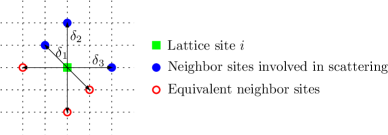
Figure 2: (Color online) The physical scenario expressed by Eq. (23).

III.2 Limiting case I: Nearest-neighbor hopping + on-site interactions

We find that the terms in the Hamiltonian Eq. (18) may now be written as

$$H_{0} =\sum_{\alpha}\Big{[}\frac{U_{\alpha}N_{\alpha}^{2}}{2N_{s}}+N_{\alpha}(\varepsilon_{0\alpha}+T_{\alpha})\Big{]}+\frac{U_{AB}N_{A}N_{B}}{N_{s}},$$ (26)

and we have introduced the basis vector

$$\phi_{\boldsymbol{k}}=[b_{{\boldsymbol{k}}A},b_{-{\boldsymbol{k}}A},b_{{\boldsymbol{k}}B},b_{-{\boldsymbol{k}}B},b^{\dagger}_{{\boldsymbol{k}}A},b^{\dagger}_{-{\boldsymbol{k}}A},b^{\dagger}_{{\boldsymbol{k}}B},b^{\dagger}_{-{\boldsymbol{k}}B}]^{\text{T}},$$ (27)

where the ’T’ superscript denotes the matrix transpose. The matrix $\check{\mathcal{M}}_{\boldsymbol{k}}$ has an $8\times 8$ structure, and reads

$$\check{\mathcal{M}}_{\boldsymbol{k}} =\begin{pmatrix}\hat{X}_{\boldsymbol{k}}&\hat{Y}_{\boldsymbol{k}}\\ \hat{Y}_{\boldsymbol{k}}&\hat{X}_{\boldsymbol{k}}\\ \end{pmatrix},$$ (28)

upon defining the auxiliary matrices:

$$\hat{X}_{\boldsymbol{k}} =\begin{pmatrix}E_{\boldsymbol{k}}^{A}&0&F_{AB}&0\\ 0&E_{\boldsymbol{k}}^{A}&0&F_{AB}\\ F_{AB}&0&E_{\boldsymbol{k}}^{B}&0\\ 0&F_{AB}&0&E_{\boldsymbol{k}}^{B}\\ \end{pmatrix},$$

$$\hat{Y}_{\boldsymbol{k}} =\begin{pmatrix}0&F_{A}&0&F_{AB}\\ F_{A}&0&F_{AB}&0\\ 0&F_{AB}&0&F_{B}\\ F_{AB}&0&F_{B}&0\\ \end{pmatrix}.$$ (29)

Upon introducing $N_{\alpha}/N_{s}=n_{\alpha}$, we may write $F_{AB}=U_{AB}\sqrt{n_{A}n_{B}},$ $F_{\alpha}=U_{\alpha}n_{\alpha}$, and $\epsilon_{\boldsymbol{k}}^{\alpha}=t_{\alpha}\sum_{\boldsymbol{\delta}}\Big{(}1-\mathrm{e}^{-\mathrm{i}{\boldsymbol{k}}\cdot\boldsymbol{\delta}}\Big{)},$ $E_{\boldsymbol{k}}^{\alpha}=\epsilon_{\boldsymbol{k}}^{\alpha}+F_{\alpha},\;\alpha=A,B.$ By undertaking a diagonalization procedure, one obtains the excitation spectrum for the condensed ground-state. Some care must be exercised in this procedure, as the new quasiparticle operators in the diagonalized basis must also satisfy the boson commutation relations. As discussed previously, it is the matrix $\check{\mathcal{M}}_{\boldsymbol{k}}\check{\sigma}_{3}$ that must be diagonalized to obtain the quasiparticle excitation energies. Evaluating the above determinant yields four distinct eigenvalues $\Lambda_{\boldsymbol{k}}=\pm\mathcal{E}_{{\boldsymbol{k}}\sigma}$, $\sigma=\pm 1$, where

$$\mathcal{E}_{{\boldsymbol{k}}\sigma}=\Big{[}\frac{\epsilon_{\boldsymbol{k}}^{A}(\epsilon_{\boldsymbol{k}}^{A}+2F_{A})+\epsilon_{\boldsymbol{k}}^{B}(\epsilon_{\boldsymbol{k}}^{B}+2F_{B})}{2}+\frac{\sigma}{2}$$

$$\times\sqrt{[\epsilon_{\boldsymbol{k}}^{A}(\epsilon_{\boldsymbol{k}}^{A}+2F_{A})-\epsilon_{\boldsymbol{k}}^{B}(\epsilon_{\boldsymbol{k}}^{B}+2F_{B})]^{2}+16F_{AB}^{2}\epsilon_{\boldsymbol{k}}^{A}\epsilon_{\boldsymbol{k}}^{B}}\Big{]}^{1/2}.$$ (30)

Note that in the limit of two decoupled Bose-Einstein condensates ($F_{AB}=0$) which are identical ($F_{A}=F_{B}=F$, $t_{A}=t_{B}=t$), we regain the well-known single-component spectrum $\mathcal{E}_{\boldsymbol{k}}=\sqrt{\epsilon_{\boldsymbol{k}}(\epsilon_{\boldsymbol{k}}+2F)}.$ The matrix $\check{D}_{\boldsymbol{k}}$ now contains the excitation spectrum and reads (the choice of the order of the eigenvalues is arbitrary)

$$\check{D}_{\boldsymbol{k}}=\text{diag}(\hat{d}_{\boldsymbol{k}},\hat{d}_{\boldsymbol{k}}),\;\hat{d}_{\boldsymbol{k}}=\text{diag}(\mathcal{E}_{{\boldsymbol{k}}+},\mathcal{E}_{{\boldsymbol{k}}-},-\mathcal{E}_{{\boldsymbol{k}}+},-\mathcal{E}_{{\boldsymbol{k}}-}).$$ (31)

Some comments are in order at this point. First of all, a similar approach to the condensed phase of a two-component Bose-Einstein condensate has been undertaken in both Ref. gu_pla_05 and liu_pra_07 . However, the final answer for the diagonalized spectrum appears to be erroneous in Ref. gu_pla_05 , where the effect of the drag (interspecies coupling $U_{AB}$) was completely disregarded in the excitation spectrum. Our results agree with the ones obtained in Ref. liu_pra_07 . The zero-temperature phase diagram for a two-component Bose-Einstein condensate on an optical lattice was analytically constructed in Ref. chen_pra_03 . Moreover, it was pointed out in Ref. oosten_pra_01 that within the framework employed here (Bogolioubov approach) one is able to obtain the criteria that demarcates the transition from a superfluid to Mott-insulator state, but one is not able to find the manifestation of this phase transition in e.g. a sharp drop of the condensate fraction.

We will now proceed to investigate the superfluid velocity in more detail. The hydrodynamic flow in a Bose-Einstein condensate, and thus the superfluid velocity, may be probed experimentally by stirring the condensate with, for instance, a blue-detuned laser beam as in Ref. onofrio_prl_00 . In the present case, we find two branches

$$\mathbf{v}_{\sigma} =\nabla_{\boldsymbol{k}}\mathcal{E}_{{\boldsymbol{k}}\sigma}|_{{\boldsymbol{k}}\to 0}.$$ (32)

Below, we consider the one-dimensional case to obtain analytically transparent results which should elucidate the basic physics. Straight-forward derivation leads to:

$$v_{\sigma}=\Big{[} \sigma a^{2}\sqrt{(t_{A}F_{A}-t_{B}F_{B})^{2}+4F_{AB}^{2}t_{A}t_{B}}$$

$$+a^{2}(t_{A}F_{A}+t_{B}F_{B})\Big{]}^{1/2}.$$ (33)

This is consistent with the sound-like spectrum of Eq. (III.2) in the long-wavelength limit $k\to 0$. Note how the superfluid velocity for each branch vanishes when the interaction parameters $U_{\alpha},U_{AB}$ in the problem are set to zero. Moreover, the superfluid velocity $\mathbf{v}_{-}$ vanishes if one of the hopping matrix elements $t_{A}$ or $t_{B}$ vanishes, in which case the interspecies interaction parameter $U_{AB}$ is not relevant in the superfluid velocity, such that $\mathbf{v}_{+}$ reduces to the superfluid velocity of a one-component Bose-Hubbard model. It is also interesting to generalize Eq. (III.2) to the case of particles moving in a continuum, by substituting

$$\epsilon_{\boldsymbol{k}}^{\alpha}\to\frac{k^{2}}{2m_{\alpha}},\;\alpha=A,B,$$ (34)

in which case the superfluid velocity takes the form

$$v_{\sigma}=\Bigg{[} \sigma\sqrt{\Big{(}\frac{F_{A}}{2m_{A}}-\frac{F_{B}}{2m_{B}}\Big{)}^{2}+\frac{F_{AB}^{2}}{m_{A}m_{B}}}$$

$$+\frac{F_{A}}{2m_{A}}+\frac{F_{B}}{2m_{B}}\Bigg{]}^{1/2}.$$ (35)

Again, the result reduces to that of a one-component Bose-Hubbard model for the case where one of the species becomes immobile, i.e. either $m_{A}$ or $m_{B}$ becomes infinite, and the superfluid velocities vanish in the non-interacting case. In the continuum picture, we may also generalize Bogolioubovs argument for the behavior of the excitations in the short- and long-wavelength limit. The limit of the long-wavelength linear sound-like spectrum is roughly demarcated by a wavevector which gives equal magnitude for the kinetic and potential energy terms in the quasiparticle dispersion relation. For component $\alpha$, the crossover wavevector $k_{c,\alpha}$ to the linear regime is given by

$$\frac{k_{c,\alpha}^{2}}{2m_{\alpha}} =n_{\alpha}(U_{\alpha}+n_{\bar{\alpha}}U_{\alpha\bar{\alpha}})$$

$$\Rightarrow k_{c,\alpha}=\sqrt{2m_{\alpha}n_{\alpha}(U_{\alpha}+n_{\bar{\alpha}}U_{\alpha\bar{\alpha}})}\sim\frac{1}{\xi_{\alpha}}.$$ (36)

where $\bar{\alpha}$ denotes the other component in the condensate while $\xi_{\alpha}$ is the coherence length. The physical picture is then that the atoms of species $\alpha$ move as free particles on short length scales compared to $\xi_{\alpha}$, while they move collectively at large length scales compared to $\xi_{\alpha}$. Some other aspects of the superfluid velocity for a two-component condensate with an energy dispersion appropriate for the continuum were considered in Ref. kravchenko_jltp_08 .

We now proceed to investigate in detail how the superfluid velocity Eq. (III.2) depends on the kinetic and potential energy terms in the problem. As seen, $v_{\sigma}$ depends on the hopping parameters $t_{\alpha}$, the intraspecies interactions $F_{\alpha}$, and the interspecies interaction $F_{AB}$. Upon choosing the parameters, we must ensure that the excitation energies remain real, as required for a stable phase of two interacting atomic species. From Eq. (III.2), one infers that the solution may become imaginary if the interaction $\gamma_{AB}^{2}$ becomes sufficiently large. The criterion for a stable coexistent phase of the condensed phase for both atomic species reads chen_pra_03

$$\gamma_{A}\gamma_{B}>\gamma_{AB}^{2}.$$ (37)

Let us first investigate how the two branches of the superfluid velocity depend on the interspecies coupling. It is convenient to rewrite Eq. (III.2) in terms of dimensionless parameters as follows:

$$v_{\sigma} =\sqrt{\zeta_{A}+\zeta_{B}+\sigma\sqrt{(\zeta_{A}-\zeta_{B})^{2}+4\rho\zeta_{A}\zeta_{B}}},$$

$$\zeta_{\alpha} =t_{\alpha}F_{\alpha}a^{2},\;\rho=\frac{F_{AB}^{2}}{F_{A}F_{B}}=\frac{\gamma_{AB}^{2}}{\gamma_{A}\gamma_{B}}.$$ (38)

It is interesting to note that for a fixed value of $\rho$, the tunnel coupling amplitudes $t_{\alpha}$ and the interaction parameters $U_{\alpha}$ play the same role. The expression for the superfluid velocity remains the same under exchange of these two energy scales. The physical regime of the normalized interspecies coupling is now $\rho\in[0,1]$, as demanded by Eq. (37). In Fig. 3, we show how the superfluid velocities in the two branches $v_{\pm}$ depend on the parameters in the problem. We give results for values of $\rho$ ranging from a weak interatomic scattering strength $(\rho=0.1)$ to a strong interaction $(\rho=0.9)$. As seen, the individual branches are not very sensitive to the value of $\rho$, but the two branches themselves differ qualitatively in their dependence on the hopping amplitudes and the potential energy. In the case of two symmetric Bose-Einstein condensates $(\zeta_{A}=\zeta_{B})=\zeta$, one obtains from Eq. (III.2) that

$$v_{\sigma}=[2\zeta(1+\sigma\sqrt{\rho})]^{1/2}.$$ (39)

The most interesting aspect of Fig. 3 is that the $v_{-}$ branch vanishes as $\rho\to 1$. This means that a very small rotation or stirring of the condensate will trigger the $\sigma=-$ branch to become a normal fluid when $\rho\to 1$.

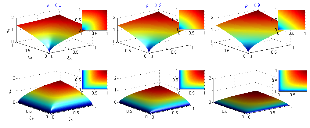
Figure 3: (Color online) Plot of the superfluid velocity for the two quasiparticle branches $v_{\pm}$. Above, we have used the dimensionless parameters $\zeta_{\alpha}=-t_{\alpha}F_{\alpha}a^{2}$ and $\rho=\gamma_{AB}^{2}/(\gamma_{A}\gamma_{B})$. The latter is a measure for the interaction between the two atomic components on the condensate.

III.3 Limiting case II: Next nearest-neighbor hopping + off-site interactions

We now go beyond the main approximation of Sec. III.2 and allow additionally for both next nearest-neighbor hopping and nearest-neighbor interactions. In this way, the interaction term in Eq. (II) becomes:

$$\frac{1}{2}\sum_{ijkl}\sum_{\alpha\beta}U_{ijkl\alpha\beta}b_{i\alpha}^{\dagger}b_{j\beta}^{\dagger}b_{k\beta}b_{l\alpha}\to\frac{1}{2}\sum_{\alpha\beta}\Big{[}\sum_{i}U_{\alpha\beta}b_{i\alpha}^{\dagger}b_{i\beta}^{\dagger}b_{i\beta}b_{i\alpha}+\sum_{i\neq j}U_{\alpha\beta}^{\prime}n_{i\alpha}n_{j\beta}\Big{]},$$ (40)

where $U_{\alpha\beta}$ and $U_{\alpha\beta}^{\prime}$ are the on-site and nearest-neighbor interactions, respectively. In order to obtain transparent analytical results, we consider the 1D case, corresponding to a trapping potential which is elongated in a ”cigar”-like shape. Proceeding in an equivalent manner as in the previous sections, we finally obtain four distinct eigenvalues $\Lambda_{\boldsymbol{k}}=\pm\mathcal{E}_{{\boldsymbol{k}}\sigma}$, $\sigma=\pm 1$, which are identical to Eq. (III.2) except that $F_{j}\to F_{\boldsymbol{k}}^{j}$, $j\in\{A,B,AB\}$, where we have defined the kinetic energy term

$$\epsilon_{\boldsymbol{k}}^{\alpha}=2t_{\alpha}[1-\cos(ka)]+2t_{\alpha}^{\prime}[1-\cos(2ka)],\;\alpha=A,B$$ (41)

and the potential energy terms

$$F_{\boldsymbol{k}}^{\alpha}=n_{\alpha}[U_{\alpha}+2U_{\alpha}^{\prime}\cos(ka)],\;\alpha=A,B$$

$$F_{\boldsymbol{k}}^{AB}=\sqrt{n_{A}n_{B}}[U_{AB}+2U_{AB}^{\prime}\cos(ka)].$$ (42)

In Eq. (41), $t_{\alpha}$ denotes the hopping parameter for nearest-neighbors while $t_{\alpha}^{\prime}$ denotes the hopping parameter for next nearest-neighbors. One now obtains the two branches of superfluid velocities which may be expressed through dimensionless quantities as follows:

$$v_{\sigma} =\sqrt{\Psi_{A}+\Psi_{B}+\sigma\sqrt{(\Psi_{A}-\Psi_{B})^{2}+4\nu\Psi_{A}\Psi_{B}}},$$ (43)

where we have defined

$$\Psi_{\alpha} =(t_{\alpha}+4t_{\alpha}^{\prime})(U_{\alpha}+2U_{\alpha}^{\prime})n_{\alpha}a^{2},$$

$$\nu =\frac{(U_{AB}+2U_{AB}^{\prime})^{2}}{(U_{A}+2U_{A}^{\prime})(U_{B}+2U_{B}^{\prime})}.$$ (44)

Note that the above equations have exactly the same form as Eq. (III.2), and that one obtains $\nu\to\rho$, $\Psi_{\alpha}\to\zeta_{\alpha}$ in the limit $\{U_{\alpha}^{\prime},U_{AB}\}\to 0$, as demanded by consistency. The stability condition for having a coexistent phase of the two superfluid branches is obtained by demanding that the eigenvalues are real, leading to the condition

$$(\epsilon_{\boldsymbol{k}}^{A}+2F_{\boldsymbol{k}}^{A})(\epsilon_{\boldsymbol{k}}^{B}+2F_{\boldsymbol{k}}^{B})>4(F_{\boldsymbol{k}}^{AB})^{2}.$$ (45)

This is a generalization of the condition $U_{A}U_{B}>U_{AB}^{2}$ that arises from the standard assumption of only nearest-neighbor hopping and on-site interactions. Assuming $\epsilon_{\boldsymbol{k}}^{\alpha}\geq 0$, we may set $\epsilon_{\boldsymbol{k}}^{\alpha}=0$ to find a more strict condition

$$\frac{[U_{AB}+2U_{AB}^{\prime}\cos(ka)]^{2}}{[U_{A}+2U_{A}^{\prime}\cos(ka)][U_{B}+2U_{B}^{\prime}\cos(ka)]}>1$$ (46)

for the phase-coexistence regime. Thus, for a strong repulsive interaction between the atomic species $A$ and $B$, one would expect that they do not coexist spatially but are instead separated into two distinct spatial regions.

III.4 Microscopic parameters and drag between superfluid components

We here derive explicit analytical expressions for the hopping and interaction parameters $t_{\alpha}$ and $U_{\alpha\beta}$ in our model. We will consider nearest-neighbor hopping and an optical lattice with intersite distance $a$. Our results are derived for the three-dimensional case, but are written down in a form which may be easily generalized to one or two dimensions.

Starting from the definitions in Eq. (II), we obtain

$$U_{\alpha\beta}=\gamma_{\alpha\beta}\prod_{j}\sqrt{\frac{m_{\alpha}m_{\beta}\tilde{\omega}_{j\alpha}\tilde{\omega}_{j\beta}}{\pi(m_{\alpha}\tilde{\omega}_{j\alpha}+m_{\beta}\tilde{\omega}_{j\beta})}},$$ (47)

which is consistent with Eq. (9) in Ref. liu_pra_07 . The definition of $\tilde{\omega}_{j\alpha}$ was given in Eq. (II). Above, $j\in\{x,y,z\}$. Now, we present a derivation of the hopping term upon taking fully into account the trapping potential, which has been neglected in the literature so far. This is appropriate in a situation where the trapping potential has been turned off, allowing the condensate to expand very slowly. Inserting the potentials and the Wannier functions into Eq. (II), we obtain

$$t_{\alpha} =-\prod_{j}\sqrt{\frac{m_{\alpha}\tilde{\omega}_{j\alpha}}{\pi}}\int_{-\infty}^{\infty}d\boldsymbol{r}\mathrm{e}^{-\boldsymbol{p}_{\alpha}\cdot\tilde{\boldsymbol{R}}(0)}$$

$$\times\Big{[}-\frac{\nabla^{2}}{2m_{\alpha}}+\tilde{\boldsymbol{V}}_{\alpha}\cdot\tilde{\boldsymbol{R}}(0)\Big{]}\mathrm{e}^{-\boldsymbol{p}_{\alpha}\cdot\tilde{\boldsymbol{R}}(a)},$$ (48)

where we have defined

$$\tilde{\boldsymbol{R}}(a) =\sum_{j}(j-a)^{2}\boldsymbol{j},\;\boldsymbol{p}_{\alpha}=(m_{\alpha}/2)\sum_{j}\tilde{\omega}_{j\alpha}\boldsymbol{j}$$

$$\tilde{\boldsymbol{V}}_{\alpha} =(m_{\alpha}/2)\sum_{j}(\omega_{j}^{2}+2V_{j}k_{j}^{2}/m_{\alpha})\boldsymbol{j}.$$ (49)

After a shift of variables, we arrive at

$$t_{\alpha}=-\prod_{j}\mathrm{e}^{-(m_{\alpha}\tilde{\omega}_{j\alpha}a^{2}/4)}\sum_{j^{\prime}}\tilde{\omega}_{j^{\prime}\alpha}/2.$$ (50)

The ratio of the interaction term and the hopping term may now be evaluated straight-forwardly for any choice of microscopic parameters. Experimentally, it is possible to tune lattice parameters $V_{0}$ and $\lambda$ through the laserlight setting up the optical potential. Defining the atom recoil energy

$$E_{R,\alpha}=k^{2}/2m_{\alpha}=2\pi^{2}/(m_{\alpha}\lambda^{2}),$$ (51)

one may then define the tunable parameter

$$s\equiv\frac{V_{0}}{E_{R,A}}$$ (52)

which captures the effect of both the lattice well depth $V_{0}$ and the lattice constant $a=\lambda/2$. We simply denote $E_{R,A}\equiv E_{R}$ from now on. For later use, we note that for a cubic lattice and in the absence of a trapping potential, we obtain the relations

$$\frac{t_{\alpha}}{E_{R}} =3\mathrm{e}^{-3\pi^{2}\sqrt{sm_{\alpha}/m_{A}}/4}\sqrt{sm_{A}/m_{\alpha}},$$

$$\frac{U_{\alpha}}{E_{R}} =\frac{a_{\alpha}}{\lambda}\frac{2}{\pi}\frac{m_{A}}{m_{\alpha}}(2\pi\sqrt{sm_{\alpha}/m_{A}})^{3/2},$$

$$\frac{U_{AB}}{E_{R}} =\frac{a_{AB}}{\lambda}\frac{1}{\pi}(1+m_{A}/m_{B})\Big{(}\frac{4\pi\sqrt{s}}{1+\sqrt{m_{A}/m_{B}}}\Big{)}^{3/2}.$$ (53)

upon choosing a positive sign for the hopping parameters. This fully determines the Bose-Hubbard parameters $t_{\alpha}$ and $U_{\alpha\beta}$ for a given set of microscopic parameters. To access the physically allowed regime of $a_{AB}$, we define

$$\eta=\frac{\gamma^{2}_{AB}}{\gamma_{A}\gamma_{B}},\;\eta\in[0,1).$$ (54)

We plot in Fig. 4 the Bose-Hubbard parameters as a function of the lattice well depth $s$ for the case of symmetric $(m_{A}/m_{B}=1.0)$ and asymmetric $(m_{A}/m_{B}=0.5)$ two-component condensate. Moreover, $a_{\alpha}/\lambda=10^{-3}$, corresponding to a scattering length of a few nm for a typical experiment. As seen, the hopping amplitude becomes comparable to the interaction term only for optical lattice potentials $V_{0}\sim E_{R}$ yielding $s\sim 1$. We do not consider here very weak lattice potentials satisfying $s\ll 1$, since the tight-binding model employed in the present paper no longer remains valid.

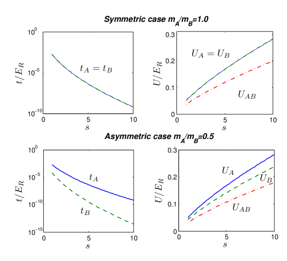
Figure 4: (Color online) Plot of the hopping and interaction parameters in the Bose-Hubbard model as a function of the trap depth $s=V_{0}/E_{R}$.

As a practical application of our results for the excitation energies as well as the relation between the Bose-Hubbard parameters and microscopic parameters, we now study the magnitude of the intercomponent drag coefficient $\rho_{d}$ in a uniform two-component BEC. In particular, we investigate what values $\rho_{d}$ may realistically take for a relevant choice of microscopic parameters. The drag stems from a transfer of motion between the supercurrents for each component as a result of the interaction $\gamma_{AB}$, and vanishes in the case of two decoupled BECs. The free energy for a uniform two-component Bose-Einstein condensate may be written as andreev_bashkin

$$F=F_{0}+V[\rho_{A}\boldsymbol{v}_{A}^{2}+\rho_{B}\boldsymbol{v}_{B}^{2}-\rho_{d}(\boldsymbol{v}_{A}-\boldsymbol{v}_{B})^{2}]/2,$$ (55)

where $F_{0}$ contains terms independent of the superfluid velocities $\boldsymbol{v}_{i}$ for the two components and $V$ is the volume of the system. The terms $\rho_{j}$, $j\in A,B$ represent the mass densities of the two components.

In Ref. fil_pra_05 , an explicit expression was derived for the intercomponent drag $\rho_{d}$ for the case of small superfluid velocities (much smaller than the critical ones) in the continuum limit, i.e. with free-boson dispersion relations $\epsilon_{{\boldsymbol{k}}}^{\alpha}=k^{2}/2m_{\alpha}$. However, the drag between components on an optical lattice remains to be investigated. In what follows, we shall calculate $\rho_{d}$ as a function of the microscopic parameters in the problem. This is accomplished by virtue of our analytical expressions for both the quasiparticle energies (Sec. III.2) and the parameters in the effective Bose-Hubbard Hamiltonian derived previously in this section. We here focus on the zero-temperature case, i.e. far away from the critical temperature, where our mean-field approach should be viable.

We now derive an analytical expression for $\rho_{d}$ from the microscopic Hamiltonian determined by Eqs. (18), (26), (27), (28), (III.2). Our strategy is to let ${\boldsymbol{k}}\to{\boldsymbol{k}}-m_{\alpha}\boldsymbol{v}_{\alpha}$ in the Hamiltonian, leading to the Doppler-shifted energies

$$\epsilon_{\boldsymbol{k}}^{\alpha}\to\epsilon_{\boldsymbol{k}}^{\alpha}-m_{\alpha}\boldsymbol{v}_{\alpha}\cdot\nabla_{\boldsymbol{k}}\epsilon_{\boldsymbol{k}}^{\alpha}.$$ (56)

The energy eigenvalues may then be solved by expanding the characteristic polynomial in orders of $\boldsymbol{v}_{\alpha}$, along the lines of herland_diplom . At zero temperature, one obtains the following expression for the drag coefficient:

$$\rho_{d}=\frac{4m_{A}m_{B}t_{A}t_{B}}{N_{x}N_{y}N_{z}a}\sum_{\boldsymbol{k}}^{\prime}\frac{F_{AB}^{2}\epsilon_{\boldsymbol{k}}^{A}\epsilon_{\boldsymbol{k}}^{B}\sin^{2}(k_{x}a)}{\mathcal{E}_{{\boldsymbol{k}},+}\mathcal{E}_{{\boldsymbol{k}},-}(\mathcal{E}_{{\boldsymbol{k}},+}+\mathcal{E}_{{\boldsymbol{k}},-})^{3}}.$$ (57)

Just like in the continuum limit treated in Ref. fil_pra_05 , we find that the drag coefficient is independent of the sign of the intercomponent scattering $F_{AB}$. It is also seen that Eq. (57) is always positive, $\rho_{d}>0$. Our results Eq. (57) may thus be considered as a generalization of the drag coefficient in Ref. fil_pra_05 to an optical lattice scenario.

We now proceed to investigate the behavior of the drag coefficient numerically on a $50\times 50\times 50$ cubic lattice $(N_{j}=50,\;V_{j}=V_{0}),\;j=\{x,y,z\}$, which corresponds to the experimental setup of Ref. greiner_nature_02 . Moreover, we fix $n_{A}=n_{B}=\sqrt{2}$, corresponding to an incommensurate filling as demanded for the superfluid phase. Let us define the normalized and dimensionless drag coefficient $\rho_{d}/\rho_{0}$, where $\rho_{0}=m_{A}N_{A}/V$. For a fixed intracomponent interaction strength $a_{\alpha}$, the drag coefficient will thus depend on the strength of the intercomponent scattering $\eta$, the mass ratio $m_{A}/m_{B}$, and the lattice well depth $s$. These microscopic parameters also determine the Bose-Hubbard parameters $t_{\alpha}$ and $U_{\alpha\beta}$ through Eq. (III.4). We present the dependence of $\rho_{d}/\rho_{0}$ on $m_{A}/m_{B}$ and $s$ in Fig. 5 for both a weak ($\eta=0.2$) and strong ($\eta=0.8$) intercomponent scattering.

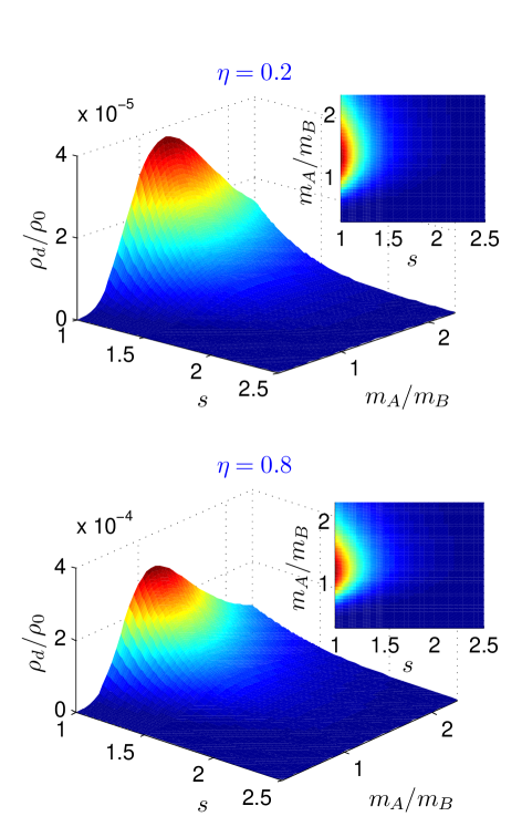
Figure 5: (Color online) Contour plot of the normalized drag coefficient $\rho_{d}/\rho_{0}$ as a function of the mass ratio $m_{A}/m_{B}$ and the lattice well depth $s$. Two different values of $\eta$ have been used, corresponding to weak ($\eta=0.2$) and strong ($\eta=0.8$) intercomponent scattering.

Qualitatively, it is seen that the plots are similar. With increasing lattice well depth $s$, the drag coefficient quickly diminishes in size. It is interesting to note that the drag coefficient is at its largest for a mass ratio $m_{A}/m_{B}\sim 1$, regardless of the value of $s$. This suggests that the velocity-drag effect between the components becomes most efficient when they have similar masses, which is reasonable. If $\rho_{d}\neq 0$, it is possible that the superfluid motion of one component induces a supercurrent in the other component purely by a drag effect, since the expressions for the supercurrents $\boldsymbol{j}_{\alpha}$ may be written as andreev_bashkin :

$$\boldsymbol{j}_{A}=(\rho_{A}-\rho_{d})\boldsymbol{v}_{A}+\rho_{d}\boldsymbol{v}_{B},\;\boldsymbol{j}_{B}=(\rho_{B}-\rho_{d})\boldsymbol{v}_{B}+\rho_{d}\boldsymbol{v}_{A}.$$ (58)

Thus, one may have $\boldsymbol{j}_{\alpha}\neq 0$ even with $\boldsymbol{v}_{\alpha}=0$.

We end this section by briefly commenting on the positivity of $\rho_{d}$ that we find. In previous works on two-component Bose condensates, a negative drag has been found numerically in Monte Carlo computations kaurov_prl_05 , and starting from such a negative value, highly unusual vortex states in a rotating multi-component Bose condensate, have been predicted which have no counterpart in the case $\rho_{d}>0$ dahl_prl_09 . In particular, a superfluid bosonic density wave, corresponding to a vortex system which has the characteristics of a liquid and a solid at the same time, has been reported dahl_prl_09 . Therefore, a negative drag has extremly important ramifications for the physics of these systems. Physically, a positive drag coefficient means, by virtue of Eq. 58, that a superfluid flow in one component of the condensate induces a co-directed, not counter-directed, flow in the other component. It should be noted that the negative drag reported in Ref. kaurov_prl_05, was obtained in a limit where the bosons on the optical lattice were very strongly interacting (essentially the hard-core boson limit) and the system was close to half-filling. Under such circumstances, one may expect a backflow of one species of bosons when a boson of one component hops from one lattice site to another site occupied by the other component. Our approach, on the other hand, is essentially a weak-coupling approach which cannot capture such physics, and this issue warrants further investigation using more suitable strong-coupling approaches.

IV Summary

In conclusion, we have investigated the excitation spectrum, superfluid velocity, and inter-component drag-coefficient for a two-component Bose-Einstein condensate on an optical lattice. We have derived analytical expressions for the excitation energies for arbitrary hopping and interaction between sites in Eqs. (24) and (III.1). We have investigated the excitation spectrum, superfluid velocity, and phase-separation condition in more detail for two important limiting cases of the general expressions. The critical superfluid velocity may be probed experimentally by using e.g. a laser as a macroscopic object to stir the hydrodynamic flow in the two-component Bose-Einstein condensate. Moreover, we have derived an analytical expression for the drag coefficient between the components when the condensate resides on an optical lattice in a weak-coupling approximation and found that it is always positive. This means that drag induces co-directed flows of superfluid components, and not counter-flows, in the weak-coupling limit. We find that the transfer of motion from one supercurrent to another becomes most efficient for a mass ratio close to one for the two components, regardless of the lattice well depth or the intercomponent scattering strength.

References

• (1) F. Dalfovo, S. Giorgini, L. P. Pitaevskii, and S. Stringari, Rev. Mod. Phys. 71, 463 (1999).
• (2) A. J. Leggett, Rev. Mod. Phys. 73, 307 (2001).
• (3) O. Morsch and M. Oberthaler, Rev. Mod. Phys. 78, 179 (2006).
• (4) D. Jaksch, C. Bruder, J. I. Cirac, C. W. Gardiner, and P. Zoller, Phys. Rev. Lett. 81, 3108 (1998).
• (5) G. Mazzarella, S. M. Giampaolo, and F. Illuminati, Phys. Rev. A 73, 013625 (2006).
• (6) G.-H. Chen and Y.-S. Wu, Phys. Rev. A 67, 013606 (2003).
• (7) D. V. Fil and S. I. Shevchenko, Phys. Rev. A 72, 013616 (2005).
• (8) V. M. Kaurov, A. B. Kuklov, and A. E. Meyerovich, Phys. Rev. Lett. 95, 090403 (2005).
• (9) E. K. Dahl, E. Babaev, S. Kragset, and A. Sudbø, Phys. Rev. B 77, 144519 (2008); E. K. Dahl, E. Babaev, and A. Sudbø, Phys. Rev. B 78, 144510 (2008).
• (10) E. K. Dahl, E. Babaev, and A. Sudbø, Phys. Rev. Lett., 101, 255301 (2008).
• (11) A. F. Andreev and E. P. Bashkin, Zh. Eksp. Teor. Fiz. 69, 319 (1975).
• (12) X. P. Liu, Phys. Rev. A 76, 053615 (2007).
• (13) J. Gu, Y.-P. Zhang, Z.-D. Li, J.-Q. Liang, Phys. Lett. A 335, 310 (2005).
• (14) D. van Oosten, P. van der Straten, and H. T. C. Stoof, Phys. Rev. A 63, 053601 (2001).
• (15) R. Onofrio, C. Raman, J. M. Vogels, J. R. Abo-Shaeer, A. P. Chikkatur, and W. Ketterle, Phys. Rev. Lett. 85, 2228 (2000).
• (16) L. Yu Kravchenko and D. V. Fil, J. Low. Temp. Phys. 150, 612 (2008).
• (17) S. M. Giampaolo, F. Illuminati, G. Mazzarella, and S. De Siena, Phys. Rev. A 70, 061601 (2004)
• (18) E. V. Herland, M. S. thesis, Norwegian University of Science and Technology, 2008.
• (19) M. Greiner, O. Mandel, T. Esslinger, T.W. H nsch, and I. Bloch, Nature 415, 39 (2002).