Exact quantum dissipative dynamics under external time–dependent fields driving

Abstract

Exact and nonperturbative quantum master equation can be constructed via the calculus on path integral. It results in hierarchical equations of motion for the reduced density operator. Involved are also a set of well–defined auxiliary density operators that resolve not just system–bath coupling strength but also memory. In this work, we scale these auxiliary operators individually to achieve a uniform error tolerance, as set by the reduced density operator. An efficient propagator is then proposed to the hierarchical Liouville–space dynamics of quantum dissipation. Numerically exact studies are carried out on the dephasing effect on population transfer in the simple stimulated Raman adiabatic passage scheme. We also make assessments on several perturbative theories for their applicabilities in the present system of study.

1 Introduction

The central problem of quantum dissipation theory is to study the dynamics of quantum system embedded in quantum thermal bath. The primary quantity of interest here is the reduced density operator, $\rho(t)\equiv{\rm tr}_{\mbox{\tiny B}}\rho_{\rm T}(t)$, after the bath degrees of freedom are all traced out from the total composite density operator. Due to its fundamental importance, quantum dissipation theory has remained as an active topic in diversified fields [1-10]. The challenge here, from both formulation and numerical aspects, is nonperturbative dissipation, with multiple time scales of memory, under time–dependent external field driving.

For Gaussian stochastic force, the influence of bath on system can be characterized by force–force correlation functions. Exact formalism had then been established via the Feynman–Vernon influence functional approach [1-5]. Direct numerical integration methods, based on discretization of the path integral and summation up of the memory correlated terms, have been put forward such as the quasi-adiabatic propagator method [11-14] or the real-time quantum Monte Carlo scheme [15-19].

The alternative is the differential approach, especially in a linear form to maximize the numerical advantage. It has also the advantage in the study of various dynamics such as the spectroscopic or control problems [20]. The calculus–on–path–integral (COPI) method is hence proposed to construct the differential counterpart of the path integral theory, reported as the hierarchical equations of motion (HEOM) formalism [21-30]. This formalism can also be derived via the stochastic description of quantum dissipation [31-35]. The COPI algorithm provides a unified approach to the influence of quantum environment ensembles, either canonical or grand canonical, and either bosonic or fermionic [28, 29]. The COPI algorithm also takes into account the combined effects of multiple memory time scales, system–bath coupling strengths, and system anharmonicity. The resulting HEOM formalism is therefore nonperturbative in nature, and always converges in principle. Moreover, the HEOM formalism is exact, not just for its propagation equivalent to the path integral theory, but also for the fact that the initial correlations between system and bath can now be incorporated by the steady–state solutions to the HEOM, before external time–dependent fields taking effect. Recently, we have further developed a numerical efficient filtering method for the propagation of the HEOM [36, 37].

In this work, we report a HEOM–based study on population transfer with dephasing in the scheme of stimulated Raman adiabatic passage (STIRAP) [38]. The laser control of dissipative systems has been addressed extensively [39-49], but mostly on the basis of weak dissipation treatment. The correlated influence of driving and dissipation is often important, as demonstrated previously [50, 51]. With the aid of the numerically exact results, we analyze the dephasing effects on transfer dynamics in relation to the STIRAP mechanism and examine some second–order quantum dissipation theories for their applicabilities in the systems of study.

The remainder of paper is organized as follows. We present the HEOM formalism together with comments on its numerical implementation in Sec. 2, and the derivations in Appendix. In Sec. 3, we study the dephasing effect on population transfer dynamics in the STIRAP scheme. We report the numerically exact results via the HEOM formalism, followed by discussions in relation to the STIRAP mechanism. In Sec. 4, we present the details of numerical performance of the HEOM results, and make concrete assessments on several approximated quantum dissipation theories. Finally we conclude the paper.

2 Hierarchical equations of motion formalism for quantum dissipation

2.1 Description of stochastic bath coupling

The total system–plus–bath Hamiltonian can be written in general as

$$\qquad H_{\rm T}=H(t)+h_{\mbox{\tiny B}}-\sum_{a}Q_{a}\hat{F}_{a}.$$ (1)

The last term denotes the multi-mode system–bath interactions. The involving system operators $\{Q_{a}\}$ are called the dissipative modes, through which the generalized Langevin forces $\{\hat{F}_{a}(t)=e^{ih_{\mbox{\tiny B}}t}\hat{F}_{a}e^{-ih_{\mbox{\tiny B}}t}\}$ from the bath ($h_{\mbox{\tiny B}}$) act on the system. For convenience, let the dissipative modes be dimensionless. The time dependence in the system $H(t)$ arises from external driving fields. Throughout this paper, we denote the inverse temperature $\beta\equiv 1/(k_{\mbox{\tiny B}}T)$ and set $\hbar\equiv 1$.

We treat the Langevin forces as Gaussian stochastic processes. Therefore their effects on the system are completely characterized by the correlation functions,

$$\qquad C_{ab}(t-\tau)=\langle\hat{F}_{a}(t)\hat{F}_{b}(\tau)\rangle_{\mbox{\tiny B}}.$$ (2)

Here, $\langle\hat{O}\,\rangle_{\mbox{\tiny B}}\equiv{\rm tr}_{\mbox{\tiny B}}(\hat{O}\rho^{\rm eq}_{\mbox{\tiny B}})$ denotes the thermodynamics average over the canonical ensembles of the bosonic bath. The correlation functions satisfy the symmetry and detailed–balance relations, or equivalently the fluctuation–dissipation theorem [3, 20]:

$$\qquad C_{ab}(t)=\frac{1}{\pi}\int_{-\infty}^{\infty}\!d\omega\,\frac{e^{-i\omega t}J_{ab}(\omega)}{1-e^{-\beta\omega}}\,,$$ (3)

with $J_{ab}(\omega)=-J_{ba}(-\omega)=J_{ba}^{\ast}(\omega)$ being the bath spectral density functions. The HEOM formalism requires $C_{ab}(t)$ be expanded in certain series form, so that the hierarchy can be constructed via consecutive time derivatives on path integral. Various schemes [22, 28, 52, 53] have been proposed to expand $C_{ab}(t)$ in exponential series, on the basis of analytical continuation evaluation of Eq. (3). In particular, the hybrid scheme that also exploits quadrature integration method is applicable for arbitrary spectral density functions [30].

For simplicity we set $C_{ab}(t)=C_{aa}(t)\delta_{ab}$. In this case the contributions from different dissipative modes $\{Q_{a}\}$ are additive. Without loss of generality, we present the formalism explicitly only for the single–dissipative–mode case, $Q_{a}=Q$. We thus omit the index $a$ for clarity of formulation. We also adopt the super-Drude model,

$$\qquad J(\omega)=\frac{\eta\omega}{[(\omega/\gamma)^{2}+1]^{2}}\,.$$ (4)

The corresponding correlation function can be analytically evaluated as [20, 28, 53]

$$\qquad C(t\geq 0)=[\nu+(\bar{\nu}_{r}+i\bar{\nu}_{i})\,\gamma t]e^{-\gamma t}+\sum_{m=1}^{M}\check{\nu}_{m}e^{-\check{\gamma}_{m}t}+\delta C(t).$$ (5)

All coefficients here are real and given in Appendix [cf. Eqs. (25) and (26)]. The first term arises from pole of the spectral density function, which is of rank two. The second term is from the Matsubara poles, with $\check{\gamma}_{m}\equiv 2\pi m/\beta$ being the Matsubara frequency. The last term is the Matsubara residue, which would approach to zero if $M\rightarrow\infty$. In this work, we adopt the Markovian residue ansatz [25, 35], i.e., $\check{\gamma}_{m}e^{-\check{\gamma}_{m}t}\big{|}_{m>M}\approx\delta(t)$; thus,

$$\qquad\delta C(t)\simeq\Delta\,\delta(t);\quad\ \ \Delta=\!\!\sum_{m=M+1}^{\infty}\frac{\check{\nu}_{m}}{\check{\gamma}_{m}}=\frac{\eta}{\beta}-\frac{\nu+\bar{\nu}_{r}}{\gamma}-\sum_{m=1}^{M}\frac{\check{\nu}_{m}}{\check{\gamma}_{m}}\,.$$ (6)

2.2 The HEOM formalism

The dynamics quantities in the HEOM formalism are the reduced density operator $\rho(t)$ and a set of auxiliary density operators (ADOs), $\{\rho_{{\sf n}}(t)\}$, that hierarchically resolve the memory contents of the bath correlation functions in the exponential series expansion of Eq. (5). The index ${{\sf n}}$ that specifies an $N^{\rm th}$–tier ADO $\rho_{{\sf n}}$ consists of a series of nonnegative integers,

$$\qquad{{\sf n}}\equiv\left\{n,n^{\prime},\bar{n},\bar{n}^{\prime},\check{n}_{1},\cdots,\check{n}_{M}\right\},\ \ {\rm with}\ \ n+n^{\prime}+\bar{n}+\bar{n}^{\prime}+\check{n}_{1}+\cdots+\check{n}_{M}=N.$$ (7)

Comparing to the reduced density operator $\rho(t)\equiv\rho_{\sf 0}(t)$ of primary interest, the specified $\rho_{{\sf n}}$ would have the order of $|\nu|^{n+n^{\prime}}\!\cdot\!|\bar{\nu}_{r}+i\bar{\nu}_{i}|^{\bar{n}+\bar{n}^{\prime}}\!\cdot\!\prod_{m=1}^{M}|\check{\nu}_{m}|^{\check{n}_{m}}$, for its dependence on the individual components of interaction bath correlation functions in the series expansion of Eq. (5). These scaling factors will be incorporated properly in the final dimensionless $\rho_{{\sf n}}$, in order to validate a filtering algorithm for the numerical efficiency of the HEOM formalism. On the other hand, the indices in the set ${\sf n}$ of Eq. (7) cover all accessible derivatives of the Feynman–Vernon influence functional; see Appendix for the details.

The final HEOM formalism is summarized as follows. It has the generic form of

$$\qquad\dot{\rho}_{{\sf n}}=-[i{\cal L}(t)+{\Gamma_{{\sf n}}}+\delta\mathcal{R}]\rho_{{\sf n}}+\rho_{\sf n}^{{}_{\{\!\rightarrow\!\}}}+\rho_{\sf n}^{{}_{\{\!-\!\}}}+\rho_{\sf n}^{{}_{\{\!+\!\}}}.$$ (8)

Here, ${\cal L}(t)\rho_{{\sf n}}\equiv[H(t),\rho_{{\sf n}}]$, which depends in general on the external driving fields; $\Gamma_{{\sf n}}$ is the damping parameter that collects all related exponents, and $\delta\mathcal{R}$ is the residue dissipation superoperator due to $\delta C(t)$. For the bath correlation function in the series expansion, Eq. (5) with Eq. (6), they are given respectively by

$$\qquad{\Gamma}_{{\sf n}}\equiv(n+n^{\prime}+{\bar{n}}+{\bar{n}}^{\prime})\gamma+\sum_{m=1}^{M}\check{n}_{m}\check{\gamma}_{m}\,,\quad\ \delta\mathcal{R}\rho_{{\sf n}}=\Delta[Q,[Q,\rho_{{\sf n}}]]\,.$$ (9)

Apparently, $\Gamma_{\sf 0}\equiv{\Gamma}_{{\sf n}}|_{N=0}=0$.

The last three terms in Eq. (8) denote how the specified $N^{\rm th}$–tier ADO $\rho_{{\sf n}}$ depends on other ADOs of the same tier, the $(N-1)^{\rm th}$–tier, and the $(N+1)^{\rm th}$–tier, respectively. For the bath correlation function in Eq. (5), they are given explicitly by

$$\qquad\rho_{\sf n}^{{}_{\{\!\rightarrow\!\}}}=\vec{\lambda}^{\,r}_{n}{\rho}_{\vec{{\sf n}}}+\vec{\lambda}^{\,i}_{n^{\prime}}{\rho}_{\vec{{\sf n}}^{\prime}}\,,$$

$$\qquad\rho_{\sf n}^{{}_{\{\!-\!\}}}=-i[Q,\lambda_{n}{\rho}_{{{\sf n}}^{-}}]+\{Q,\lambda_{n^{\prime}}{\rho}_{{{\sf n}}^{\prime-}}\}-i\Big{[}Q,\sum_{m=1}^{M}\check{\lambda}_{\check{n}_{m}}{\rho}_{{\check{{\sf n}}}_{m}^{-}}\Big{]}\,,$$ (10)

$$\qquad\rho_{\sf n}^{{}_{\{\!+\!\}}}=-i\Big{[}Q,\lambda_{n+1}{\rho}_{{{\sf n}}^{\!+}}+{\rm sign}(\bar{\nu}_{r})\!\cdot\!\bar{\lambda}^{\,r}_{\bar{n}+1}{\rho}_{\bar{{\sf n}}^{\!+}}-\bar{\lambda}^{\,i}_{\bar{n}^{\prime}+1}{\rho}_{\bar{{\sf n}}^{\prime\!+}}-\sum_{m=1}^{M}\check{\lambda}_{\check{n}_{m}+1}{\rho}_{{\check{{\sf n}}}^{\!+}_{m}}\Big{]}\,.$$

Here, $\lambda_{n}=\sqrt{n|\nu|}$ , $\check{\lambda}_{\check{n}_{m}}=\sqrt{\check{n}_{m}|\check{\nu}_{m}|}$ , $\bar{\lambda}^{\,r/i}_{n}=\sqrt{n|\bar{\nu}_{r/i}|}$ , and $\vec{\lambda}^{\,r/i}_{n}=\gamma\bar{\lambda}^{\,r/i}_{n+1}\sqrt{\bar{n}/|\nu|}$ , with the italic–font indices being from those in ${\sf n}$ of Eq. (7). The indexes variations in Eq. (10) that specify those ADOs participating in the equation of $\dot{\rho}_{{\sf n}}$ are exemplified as follows:

$$\qquad\vec{{\sf n}}\equiv\left\{n+1,n^{\prime},\bar{n}-1,\bar{n}^{\prime},\check{n}_{1},\cdots,\check{n}_{M}\right\},\quad{\sf n}^{\pm}\equiv\left\{n\pm 1,n^{\prime},\bar{n},\bar{n}^{\prime},\check{n}_{1},\cdots,\check{n}_{M}\right\}.$$ (11)

Similarly, $\vec{{\sf n}}^{\prime}$ differs from ${\sf n}$ of Eq. (7) only by changing $(n^{\prime},\bar{n}^{\prime})$ to $(n^{\prime}+1,\bar{n}^{\prime}-1)$, while $\check{{\sf n}}_{m}^{\pm}$ by changing $\check{n}_{m}$ to $\check{n}_{m}\pm 1$, and so on. Also note that ${\rho}_{\vec{{\sf n}}}$ is an $N^{\rm th}$–tier ADO, while ${\rho}_{{{\sf n}}^{\!\pm}}$ is of an $(N\pm 1)^{\rm th}$ tier, as inferred from the second identity of Eq. (7).

The initial conditions to the HEOM in the study of driven dissipative dynamics are obtained via the steady–state solutions to Eq. (8), before the time–dependent external fields interactions. For the steady–state solutions satisfying $\dot{\rho}^{\rm st}_{{\sf n}}=0$, Eq. (8) reduces to a set of linear equations, under the constraint of ${\rm Tr}\rho_{\sf 0}=1$. The resulting $\rho^{\rm st}_{{\sf n}}$ is used as the initial $\rho_{{\sf n}}(t_{0})$ to the HEOM. The initial system–bath correlations are accounted for by those nonzero initial ADOs.

2.3 Comments on numerical implementation

For the numerical HEOM propagation, we would like to have certain convenient working index scheme to track the multiple indices, denoted now as an ordered set of ${\sf n}=\{n_{1},\cdots,n_{K}\}$, that specifies $\rho_{{\sf n}}$. Here we will provide two such schemes. The number of the $N^{\rm th}$–tier ADOs, with $n_{1}+\cdots+n_{K}=N$, is $\frac{(N+K-1)!}{N!\,(K-1)!}\equiv\left[\,{}^{N}_{K}\,\right]$. In one scheme, the ADOs are arranged as $\rho_{{\sf n}}\equiv\rho_{j_{{\sf n}}}$ with $j_{{\sf n}}$ initialized by $j_{{{\sf n}}={\sf 0}}\equiv 0$ and then

$$\qquad j_{{{\sf n}}\neq{\sf 0}}=j_{n_{1}\cdots n_{K}}=\sum_{N^{\prime}=0}^{N-1}\left[\,{}^{N^{\prime}}_{K}\,\right]+\sum_{k=1}^{K}\sum_{q=0}^{N-s_{k}}\left[\,{}^{\ \ q}_{K-k}\,\right];\ \ s_{k}=1+n_{1}+\cdots+n_{k}.$$ (12)

Let $L$ be the maximum level of the hierarchical tier. The total number of the ADOs $\{\rho_{{\sf n}};0\leq N\leq L\}$ is

$$\qquad{\cal N}=\sum_{N=0}^{L}\left[\,{}^{N}_{K}\,\right]\equiv\left\{\,{}^{L}_{K}\,\right\}.$$ (13)

In another scheme, ADOs can also be arranged as $\rho_{{\sf n}}\equiv\rho_{l_{{\sf n}}}$; $l_{{\sf n}}=0,\cdots,{\cal N}-1$, with

$$\qquad l_{{\sf n}}=l_{n_{1}\cdots n_{K}}=n_{1}+\sum_{k=2}^{K}\sum_{q=1}^{n_{k}}\left\{\,{}^{L+q-(n_{k}+\cdots+n_{K})}_{\qquad k-1}\,\right\}.$$ (14)

Both schemes, Eq. (12) and Eq. (14), allow easy tracking of the coupled ADOs in the HEOM. The former [Eq. (12)] is somewhat more convenient in the filtering propagator described soon since it does not depend on $L$.

The major difficulty in implementing the HEOM formalism is its numerical tractability. The number of ADOs, ${\cal N}$ of Eq. (13), itself alone can be huge in the case of strong non-Markovian system–bath coupling and/or low temperature, as large $L$ and/or large $K$ implied. Thus, a brute–force implementation is greatly limited by the memory and central processing unit (CPU) capability of computer facility, even for a two–level system where each ADO is a $2\times 2$ matrix.

To facilitate this problem, Shi, Xu, Yan and coworkers have recently proposed an efficient numerical filtering algorithm that often reduces the effective number of ADOs by order of magnitude [36, 37]. In reality, there is usually only a very small fraction of total ADOs significant to the reduced system dynamics. To validate the accuracy–controlled numerical filtering algorithm, the present HEOM formalism has been scaled properly so that all ADOs $\{\rho_{\sf n}(t)\}$ are of a uniform error tolerance. This remarkable feature is suggested by comparing the HEOM theory with the stochastic bath interaction field approach in the case of Gaussian–Markovian dissipation [37]. The involving ADOs are just the expansion coefficients, over the normalized harmonic wave functions that are used as the basis set for resolving the diffusive bath field [37]. Our numerical HEOM propagator exploits the filtering algorithm [36]. It goes simply as follows. If a $\rho_{{\sf n}}(t)$ whose matrix elements amplitudes become all smaller than the pre–chosen error tolerance, it is set to be zero. Apparently, the filtering algorithm also automatically truncate the required hierarchy level on–the–fly during numerical propagation. By far the truncation for the Matsubara expansion still goes by checking convergency.

3 Effect of dephasing on population transfer via STIRAP

3.1 Numerical results

The STIRAP is celebrated as an efficient and robust method for population transfer [38]. It is characterized by its counterintuitive field configuration. For a three-level ${\Lambda}$–system as Fig. 1, the Stokes pulse proceeds the pump pulse, and the intermediate state remains effective in dark. The STIRAP mechanism [38] is rooted at the existence of the coherent population trapping state under the two–photon resonance condition, $\omega_{S}-\omega_{P}=\epsilon_{1}-\epsilon_{3}$, in the ${\Lambda}$–system. Dephasing destroys this condition in terms of resonance and/or the existence of coherent population trapping state. The effect of dephasing on the simple STIRAP scheme has been studied extensively, but with approximations. These include phenomenological/perturbative methods [44-46], or classical/stochastical bath treatments [47-49].

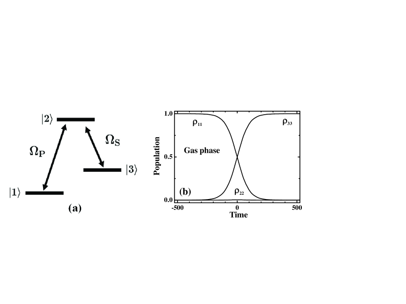
Figure 1: (a) A schematic view of the STIRAP of a three-level $\Lambda$ system. (b) Population transfer under the STIRAP scheme for the dissipation-free gas phase. The time is in the unit of $\beta$. See parameters in the text.

We revisit the dephasing effect on the simple STIRAP–based population transfer, as the exact dissipative dynamics are now established with the present HEOM formalism. We also examine three schemes of second–order approximation [20, 52-55]: (i) The Redfield theory, which neglects the correlated driving–and–dissipation effect; (ii) CS–COP, which is the conventional time–nonlocal quantum master equation, including the field–dressed dissipation contribution, and equivalent to the present HEOM truncated at the first tier; (iii) CODDE, in which the driving field–free part of dissipation superoperator is time–local, while the field–dressed part is time–nonlocal. Neglecting the latter leads it to the Redfield theory.

The total Hamiltonian under the rotating wave approximation assumes

$$\qquad H_{\rm T}(t)=\Omega_{P}(t)\hat{D}_{P}+\Omega_{S}(t)\hat{D}_{S}+\sum_{j}\Bigl{[}\frac{p_{j}^{2}}{2m_{j}}+\frac{1}{2}m_{j}\omega_{j}^{2}\Bigl{(}x_{j}-\sum_{a}\frac{c_{aj}Q_{a}}{m_{j}\omega_{j}^{2}}\Bigr{)}^{2}\Bigr{]}.$$ (15)

Here, $\hat{D}_{P}\equiv|1\rangle\langle 2|+|2\rangle\langle 1|$ and $\hat{D}_{S}\equiv|2\rangle\langle 3|+|3\rangle\langle 2|$, while $\Omega_{P}(t)$ and $\Omega_{S}(t)$ denote the Rabi frequencies of the resonant pump and Stokes fields, respectively. The dissipative mode $Q_{a}=|a\rangle\langle a|$ is responsible for dephasing. The interaction spectral density function $J_{a}(\omega)\equiv(\pi/2)\sum_{j}[c^{2}_{aj}/(m_{j}\omega_{j})]\delta(\omega-\omega_{j})$ assumes super–Drude as Eq. (4). The system Hamiltonian is then

$$\qquad H(t)=\Omega_{P}(t)\hat{D}_{P}+\Omega_{S}(t)\hat{D}_{S}+\sum_{a=1}^{3}\delta\epsilon_{a}|a\rangle\langle a|\,.$$ (16)

The Caldeira–Leggett renormalization energy [56, 57] is $\delta\epsilon_{a}=\frac{1}{\pi}\int_{0}^{\infty}\!\!d\omega\,J_{a}(\omega)/\omega=\frac{1}{4}\eta_{a}\gamma_{a}$, for the super–Drude model [Eq. (4)]. In the STIRAP configuration, it would relate to the effective detuning at short–time of the pump or Stokes field, as inferred from the analytical result of driven Brownian oscillator [20, 58].

We set the pump and Stokes fields be of same Gaussian shape, $\Omega_{P}(t+t_{P})=\Omega_{S}(t+t_{S})=A\exp[-\frac{1}{2}(wt)^{2}]$, but center them at $t_{P}=200\,\beta$ and $t_{S}=-200\,\beta$, respectively and counter-intuitively. The driving strength and inverse duration parameters are set to be $\beta A=0.1$ and $\beta w=0.005$. The corresponding dissipation–free transfer dynamics is shown in Fig. 1(b). As here the bath influence is considered to be pure-dephasing in the absence of fields, the initial system is just chosen to be completely on the $|1\rangle$ state and all the ADOs are zero. For the effect of bath, we set the coupling strength $\eta=0.64$ [cf. Eq. (4)], and consider both the Markovian and non-Markovian cases as follows.

Figure 2: Evolutions of $\rho_{33}$ and $\rho_{22}$ (in insets) via the exact HEOM (solid), CODDE (dash), CS-COP (dot) and the Redfield equation (thin-solid) for single–dissipative–mode case: (a) $Q_{1}=|1\rangle\langle 1|$ and (b) $Q_{2}=|2\rangle\langle 2|$. The system–bath coupling strength $\eta=0.64$. The parameter $\beta\gamma=5$ exemplifies the Markovian condition. The time is in the unit of $\beta$.

Figure 3: Same as Fig. 2, except the parameter $\beta\gamma=0.5$ exemplifies the non-Markovian condition. The time is in the unit of $\beta$.

Figure 4: Two-mode dissipation cases: (a) $Q_{1}=|1\rangle\langle 1|$ and $Q_{2}=|2\rangle\langle 2|$ together, and (b) $Q_{1}=|1\rangle\langle 1|$ and $Q_{3}=|3\rangle\langle 3|$ together, evaluated with $\beta\gamma=0.5$. The system–bath coupling strength $\eta=0.64$. The time is in the unit of $\beta$.

The Markovian transfer dynamics, under the influence of single dephasing mode of either $Q_{1}=|1\rangle\langle 1|$ or $Q_{2}=|2\rangle\langle 2|$, is exemplified in Fig. 2, with $\beta\gamma=5$. We observe: (i) The $Q_{1}$-mode effect shown in Fig. 2(a) leads to all three populations about $1/3$ after the driving; (ii) The $Q_{2}$-mode effect shown in Fig. 2(b) is less sensitive than its $Q_{1}$ counterpart, achieving a higher transfer efficiency, despite it is only about 0.55.

The non–Markovian transfer dynamics is exemplified in Fig. 3, with $\beta\gamma=0.5$. In comparison with the Markovian counterparts, we observe: (${\bf iii}$) The $Q_{1}$-mode case behaves about the same; (${\bf iv}$) But the $Q_{2}$-mode results in a higher transfer yield, increasing to about 0.73 via the exact calculation. We have also calculated the influences of $Q_{3}=|3\rangle\langle 3|$ for both Markovian and non-Markovian cases. The results (not shown here) are similar to those of $Q_{1}$, except for some small oscillations.

Two double–modes ($Q_{1}+Q_{2}$ and $Q_{1}+Q_{3}$ uncorrelated) non–Markovian dephasing dynamics are shown in Fig. 4(a) and (b), respectively. They are insensitive to the non–Markovian parameter, and both reach at the final equal–populations, based on the numerically exact results. Comments on the approximated schemes, the CODDE, CS–COP, and Redfield theory, presented in Figs. 2–4 will be given later; see Sec. 4.2.

3.2 Discussions

The above observations can be understood by the well–established STIRAP mechanism [38]. The $Q_{1}$–mode, which associates with the fluctuation of level $|1\rangle$, easily destroy the two–photon resonance (TPR) condition, as described at the beginning of Sec. 3. Thus, it ends up with the observed equal populations in all accessible levels by the strong fields, as consistent with the analysis in [44]. The similarity between the $Q_{3}$ and $Q_{1}$ influences is also explained. The same reason accounts further for the case of uncorrelated two modes ($Q_{1}+Q_{2}$ or $Q_{1}+Q_{3}$) dephasing, as depicted in Fig. 4. It is anticipated that when $\gamma\ll w$ (termed as the linear adiabatic limit below), the equal–population will be broken to be in favor of $|3\rangle$, due to the marginally partial fulfilment of the TPR condition.

On the other hand, the $Q_{2}$-mode is associated with the fluctuation of the intermediate level $|2\rangle$. It alone does not affect the TPR condition. However, this condition, based on the numerically exact results shown in this work, is not sufficient to retain the coherent population trapping state, chosen ad hoc earlier for the dephasing–free STIRAP scenario in Fig. 1(b). It is anticipated that the coherent population trapping state may be recovered in the aforementioned linear adiabatic limit. This is in line with the observation-(${\bf iv}$), where the non–Markovian population transfer with single $Q_{2}$-mode dephasing [Fig. 3(b)] is of higher efficiency than its Markovian counterpart [Fig. 2(b)]. The previous study based on perturbative dephasing dynamics [44] has also shown that the single $Q_{2}$-mode does not affect the transfer efficiency in the linear adiabatic limit. Nevertheless, STIRAP in the presence of complex dephasing, if 100% transfer ever achievable, would require dynamics feedback control of pump or Stokes laser frequency [59]. This would involve chirp and realize STIRAP in a nonlinear adiabatic condition, rather than the linear simplification considered here.

4 Assessments on theoretical methods and concluding remarks

4.1 Numerical performance of the HEOM formalism

Table 1: Performance of HEOM formalism with filtering.

• $10^{-6}$–filter	CPU (min)	${\cal N}_{\rm max}$ (${\cal N}$)	$L_{\rm max}$	$\kappa$	$\check{\kappa}_{1}$
  Fig. 2(b)	932	$19765$ ($8.44\times 10^{6}$)	17	0.95	1.28
  Fig. 3(b)	15	$400$ ($9.24\times 10^{4}$)	9	1.24	348
  Fig. 4(b)	266	$3664$ ($1.00\times 10^{7}$)	9	1.24	348

The numerical performance of the HEOM formalism with filtering is summarized in Table 1, for the systems reported in the three figures’ (b)-panels. The CPU time is for a single Intel(R) Xeon(R) processor@3.00GHz to calculate the exact result in each (b)-panel for the time period $-1200\,\beta<t<2000\,\beta$ with the time step $dt=0.01\beta$ using the fourth-Order Runge-Kutta propagator; ${\cal N}_{\rm max}$ denotes the largest number of active ADOs and $L_{\rm max}$ the highest tier level, ever survived in the entire time span of the numerical propagation. The filtering error tolerance is chosen to be 10^-6, following our previous work [36]. We input $M=6$ for the number of Matsubara terms being explicitly included, which has been tested to give converged results of $\rho(t)=\rho_{\sf 0}(t)$ in all calculations. The total number ${\cal N}$ of mathematical ADOs follows Eq. (13) and is given inside the parentheses. The effect of filtering is clearly seen. The number of active ADOs with filtering is insensitive to the input $M$, as long as it is large enough. In the present study, the number of active ADOs reaches ${\cal N}_{\rm max}$ only during the period about $-250\,\beta<t<500\,\beta$ and grows up or drops down dramatically outside that period with the fields turning on or getting over. Apparently, ${\cal N}_{\rm max}$ increases with the number of dissipative modes.

At least one $(L_{\rm max})^{\rm th}$–tier ADO actively participates during the HEOM propagation. Its leading contribution to the reduced density operator is of $(2L_{\rm max})^{\rm th}$ order in the system–bath interaction. Physically, ${L}_{\rm max}$ is closely related to the modulation $\kappa$-parameter [27], introduced originally by Kubo for motional narrowing problem [6]. This dimensionless parameter is determined via $\kappa\equiv\gamma/\sqrt{\nu}$, or similar, for each individual exponential component in Eq. (5). The last two columns of Table 1 are the modulation parameters $\kappa$ and $\check{\kappa}_{m=1}$ of the leading Matsubara term. The modulation $\kappa$-parameter relation to the value of $L_{\rm max}$ [27] can be clearly seen. In both the Markovian and non-Markovian cases of the present study, $\check{\kappa}_{m}=\check{\gamma}_{m}/\sqrt{|\check{\nu}_{m}|}$ monotonically increases with $m$, cf. Eq. (26). Actually, the Matsubara series truncation $M$ in Eq. (5) can be estimated via its reaching the fast modulation condition, $\check{\kappa}_{M}\gg 1$. As the temperature decreases, $\check{\kappa}_{m}$ getting smaller, and eventually cause the value of $L_{\rm max}$ be pretty large. The present HEOM construction is based on the Matsubara series expansion, which may no longer be numerically implementable in the extremely low temperature regime. Alternative expansion method such as the hybrid scheme [30] is needed to the required HEOM construction.

4.2 Assessments on three second–order approximated theories

With the exact results, we can now make concrete assessments on the three second–order approximated schemes, the Redfield theory, CS–COP, and CODDE, exploited in the numerical demonstrations. The dissipative modes $\{Q_{a}=|a\rangle\langle a|\}$ considered in Sec. 3 are all of pure dephasing, in the absence of external fields. The Redfield theory would be exact if there were no correlated driving–and–dissipation effect [20, 54]. Therefore, the non–Markovian dynamics manifest here as the correlated driving and dissipation. Apparently, the Redfield theory, by its Markovian nature, is independent of the width $\gamma$–parameter of bath spectral density. Observed is also the fact that the schemes of approximation are sensitive to the $Q_{2}$-mode rather than the $Q_{1}$- or $Q_{3}$-mode dephasing. This fact is also easily understood, by considering their relations to the STIRAP mechanism as discussed earlier. Further remarks on the approximated theories for their applicabilities in the systems of study are as follows.

The CS–COP theory [20, 53, 55] is overall most unsatisfactory, despite it contains formally a description of memory and driving–and–dissipation correlation. Even in the non–Markovian $Q_{2}$-mode case of Fig. 3(b) where it appears to be superior than the Redfield theory, the CS–COP results in a decreased transfer efficiency from its Markovian counterpart shown in Fig. 2(b). This is qualitatively contradictory to the physical anticipation, as discussed earlier.

The CODDE [20, 53, 55] appears to be the most favorable perturbation theory. It gives the best approximated transfer dynamics in all cases presented in Sec. 3, except the one to be discussed soon. Its overall superiority is also true in the driven Brownian oscillator systems [20, 51]. The CODDE is actually a modified Redfield theory, with inclusion of correlated driving–and–dissipation effects. The involving field–dressed dissipation kernel is time–nonlocal but constructed with a partial ordering resummation, rather than the chronological ordering prescription that characterizes the CS–COP [20, 53, 55].

The only exception is the Markovian $Q_{1}$–mode case shown in Fig. 2(a), where the Redfield dynamics is almost exact. The reason for this exception is also accountable. As we mentioned earlier, the non–Markovian dynamics manifest as the correlated driving and dissipation. This correlated effect diminishes in both the fast– and slow–modulation regimes, as inferred from the exact and analytical results of driven Brownian oscillator systems [58]. This conclusion can be carried over to the present system of study, as suggested here. Apparently, the identical value of $\beta\gamma=5$, adopted in the two cases of Fig. 2, acquires the fast–modulation limit for the $Q_{1}$–mode, but not yet for the $Q_{2}$–mode. In the latter case, the CODDE resumes its superiority.

4.3 Closing remarks

In summary, we have presented a hierarchical Liouville–space approach, which is exact and also quite tractable numerically, to general quantum dissipation systems under external driving fields. The auxiliary density operators are all of a uniform error tolerance, as that of the reduced density operator. We also make comments on the numerical facilitation about the multiple–index assignment and the filtering algorithm. We numerically study the dephasing effects on the population transfer, with a fixed simple STIRAP configuration, and present a concrete assessment on various approximation schemes.

Appendix. Construction of HEOM via the COPI approach

This appendix gives the details of the COPI approach to the HEOM formalism. It starts with the influence functional in path integral. Let $\{|\alpha\rangle\}$ be a basis set in the system subspace and set ${\bm{\alpha}}\equiv(\alpha,\alpha^{\prime})$ for abbreviation. Denote the evolution of reduced system density operator in the $\alpha$-representation by

$$\qquad\rho({\bm{\alpha}},t)\equiv\rho(\alpha,\alpha^{\prime}\!,t)\equiv\!\int\!d{\bm{\alpha}}_{0}\,{\cal U}({\bm{\alpha}},t;{\bm{\alpha}}_{0},t_{0})\rho({\bm{\alpha}}_{0},t_{0}).$$ (17)

Here, the reduced Liouville-space propagator is

$$\qquad{\cal U}(\bm{\alpha},t;\bm{\alpha}_{0},t_{0})=\int_{\bm{\alpha}_{0}[t_{0}]}^{\bm{\alpha}[t]}\!\!{\cal D}{\bm{\alpha}}\,e^{iS[\alpha]}{\cal F}[\bm{\alpha}]e^{-iS[\alpha^{\prime}]}.$$ (18)

The effects of bath on the reduced system are contained completely in the influence functional ${\cal F}$. For Gaussian stochastic forces $\{\hat{F}_{a}(t)\}$ from fluctuating bath, it assumes the Feynman–Vernon form [1], which can be recast as [27-29]:

$$\qquad{\cal F}[\bm{\alpha}]=\exp\Bigl{\{}-\int_{t_{0}}^{t}\!\!d\tau\,\sum_{a}{\cal A}_{a}[\bm{\alpha}(\tau)]\,{\cal B}_{a}(\tau;\{\bm{\alpha}\})\Bigr{\}},$$ (19)

with

$$\qquad{\cal A}_{a}[\bm{\alpha}(t)]=Q_{a}[\alpha(t)]-Q_{a}[\alpha^{\prime}(t)],$$ (20)

$$\qquad{\cal B}_{a}(t;\{\bm{\alpha}\})=B_{a}(t;\{\alpha\})-B^{\prime}_{a}(t;\{\alpha^{\prime}\}),$$ (21)

and

$$\qquad\eqalign{B_{a}(t;\{\alpha\})&\equiv\sum_{b}\int_{t_{0}}^{t}\!d\tau\,C_{ab}(t-\tau)Q_{b}[\alpha(\tau)],\cr B^{\prime}_{a}(t;\{\alpha^{\prime}\})&\equiv\sum_{b}\int_{t_{0}}^{t}\!d\tau\,C^{\ast}_{ab}(t-\tau)Q_{b}[\alpha^{\prime}(\tau)].}$$ (22)

Here, $C_{ab}(t)$ is the bath correlation functions, defined by Eq. (2). The functional ${\cal A}_{a}$ [Eq. (20)] depends only on the local time and its operator level form is just the commutator of the dissipative mode $Q_{a}$.

The functional ${\cal B}_{a}$ [Eq. (21)] does however contain memory, which is to be resolved via the COPI algorithm of consecutive time derivatives on all memory–contained functionals. To construct a close set of HEOM via the COPI algebra, it needs a proper expansion of $C_{ab}(t)$ such as the exponential series, while maintaining the fluctuation–dissipation theorem of Eq. (3). A super–Drude parametrization scheme and the resulted HEOM formalism have been presented in our previous work [28]. A hybrid scheme, exploiting the analytical continuation and quadrature integration methods to evaluate the fluctuation–dissipation theorem, has also been proposed [30].

To illustrate the COPI algorithm, consider the super-Drude model,

$$\qquad J_{ab}(\omega)=\frac{\eta_{ab}\omega+i\eta^{\prime}_{ab}\omega^{2}}{[(\omega/\gamma_{ab})^{2}+1]^{2}}\,.$$ (23)

The parameters are all real and satisfy the symmetry relations of $\eta_{ab}=\eta_{ba},\ \gamma_{ab}=\gamma_{ba}$, and $\eta^{\prime}_{ab}=-\eta^{\prime}_{ba}$, as inferred from the symmetric relations implied in $J_{ab}(\omega)$. The resulting correlation functions via Eq. (3) are

$$\qquad C_{ab}(t\geq 0)=[(\nu^{ab}_{r}+i\nu^{ab}_{i})+(\bar{\nu}^{ab}_{r}+i\bar{\nu}^{ab}_{i})\,\gamma_{ab}t]e^{-\gamma_{ab}\,t}+\sum_{m=1}^{M}\check{\nu}_{m}^{ab}e^{-\check{\gamma}_{m}t}+\delta C_{ab}(t).$$ (24)

The second term arises from the Matsubara poles, with $\check{\gamma}_{m}=2\pi m/\beta$ the Matsubara frequencies, and $\check{\nu}^{ab}_{m}=-i(2/\beta)J_{ab}(-i\check{\gamma}_{m})=(\nu^{ab}_{m})^{\ast}$ is real, as inferred from the symmetry relation of the spectral density function in analytical continuation. The first term arises from pole of the spectral density function of rank 2. The involving coefficients are summarized as follows [20, 28, 53].

$$\qquad\eqalign{\nu^{ab}_{i}=\eta^{\prime}_{ab}\gamma_{ab}^{3}/4,\quad\bar{\nu}^{ab}_{i}=-{\frac{1}{4}}(\eta_{ab}+\eta^{\prime}_{ab}\gamma_{ab})\gamma_{ab}^{2}\,,\quad\bar{\nu}^{ab}_{r}=-\bar{\nu}^{ab}_{i}\cot(\beta\gamma_{ab}/2),\cr\nu^{ab}_{r}=-\nu^{ab}_{i}\cot(\beta\gamma_{ab}/2)-\bar{\nu}^{ab}_{i}(\beta\gamma_{ab}/2)\csc^{2}(\beta\gamma_{ab}/2)\,,}$$ (25)

and

$$\qquad\check{\nu}^{ab}_{m}=-\frac{2(\eta_{ab}\check{\gamma}_{m}+\eta^{\prime}_{ab}\check{\gamma}_{m}^{2})}{\beta[(\check{\gamma}_{m}/\gamma_{ab})^{2}-1]^{2}}\equiv\check{\gamma}^{2}_{m}\check{\eta}^{ab}_{m}\,,{\rm\ with\ \ }\check{\eta}^{ab}_{m}=-\frac{(\eta_{ab}+\eta^{\prime}_{ab}\check{\gamma}_{m})/(m\pi)}{[(\check{\gamma}_{m}/\gamma_{ab})^{2}-1]^{2}}.$$ (26)

The residue $\delta C_{ab}(t)$ can be approximated via the Markovian ansatz, i.e., $\delta C_{ab}(t)\simeq\Delta_{ab}\delta(t)$; cf. Eq. (6).

To proceed we denote for every distinct exponent terms in Eq. (24),

$$\qquad\eqalign{&B_{ab}(t;\{\alpha\})\equiv\int_{t_{0}}^{t}\!d\tau\,e^{-\gamma_{ab}(t-\tau)}Q_{b}[\alpha(\tau)],\cr&\bar{B}_{ab}(t;\{\alpha\})\equiv\int_{t_{0}}^{t}\!d\tau\,\gamma_{ab}(t-\tau)e^{-\gamma_{ab}(t-\tau)}Q_{b}[\alpha(\tau)],\cr&\check{B}^{a}_{m}(t;\{\alpha\})\equiv\sum_{b}\check{\eta}^{ab}_{m}\int_{t_{0}}^{t}\!d\tau\,e^{-\check{\gamma}_{m}(t-\tau)}Q_{b}[\alpha(\tau)];\quad m=1,\cdots,M.}$$ (27)

They are related to the influence generating functionals as [cf. Eq. (22)]

$$\qquad\eqalign{&{\cal B}_{ab}\equiv-i(B_{ab}-B^{\prime}_{ab}),\qquad{\cal B}^{\prime}_{ab}\equiv B_{ab}+B^{\prime}_{ab},\cr&\bar{\cal B}_{ab}\equiv-i({\bar{B}}_{ab}-{\bar{B}}^{\prime}_{ab}),\qquad\bar{\cal B}^{\prime}_{ab}\equiv{\bar{B}}_{ab}+{\bar{B}}^{\prime}_{ab},\cr&\check{\cal B}^{a}_{m}\equiv-i(\check{B}^{a}_{m}-\check{B}^{\prime a}_{m});\qquad\ \ m=1,\cdots,M.}$$ (28)

Now we define the auxiliary density operators (ADOs) via

$$\qquad\rho_{\sf n}(t)\equiv{\cal U}_{\sf n}(t,t_{0})\rho(t_{0}),$$ (29)

where

$$\qquad{\cal U}_{\sf n}(\bm{\alpha},t;\bm{\alpha}_{0},t_{0})\equiv\int_{\bm{\alpha}_{0}[t_{0}]}^{\bm{\alpha}[t]}\!\!{\cal D}{\bm{\alpha}}\,e^{iS[\alpha]}{\cal F}_{\sf n}[\bm{\alpha}]e^{-iS[\alpha^{\prime}]},$$ (30)

with

$$\qquad{\cal F}_{\sf n}=s_{\sf n}\Bigl{\{}\prod_{a,b}\bigl{[}({\cal B}_{ab})^{n_{ab}}({\cal B}^{\prime}_{ab})^{n^{\prime}_{ab}}(\bar{\cal B}_{ab})^{\bar{n}_{ab}}(\bar{\cal B}^{\prime}_{ab})^{\bar{n}^{\prime}_{ab}}\bigr{]}\prod_{a,m}\bigl{(}\check{\cal B}^{a}_{m}\bigr{)}^{\check{n}_{m}^{a}}\Bigr{\}}{\cal F}.$$ (31)

The scaling factor $s_{\sf n}$ is defined as

$$\qquad s_{{\sf n}}=\Big{\{}\prod_{a,b}\frac{|\nu_{r}^{ab}|^{n_{ab}}|\nu_{i}^{ab}|^{n^{\prime}_{ab}}|\bar{\nu}_{r}^{ab}|^{\bar{n}_{ab}}|\bar{\nu}_{i}^{ab}|^{\bar{n}^{\prime}_{ab}}}{{n_{ab}}!\,{n^{\prime}_{ab}}!\,{\bar{n}_{ab}}!\,{\bar{n}^{\prime}_{ab}}!\,}\Big{\}}^{\frac{1}{2}}\prod_{a,m}\frac{\check{\gamma}_{m}^{\check{n}_{m}^{a}}}{\sqrt{\check{n}_{m}^{a}!}}.$$ (32)

The ADOs $\{\rho_{\sf n}\}$ defined in this way are dimensionless and possess uniform error tolerance to support the filtering method, as described in Sec. 2.3. Since $\eta^{\prime}_{aa}=0$ hence $\nu^{aa}_{i}=0$, we set $\nu^{aa}_{i}\equiv\nu^{aa}_{r}$ for the scaling factor $s_{{\sf n}}$ of Eq. (32) and hereafter. The index set for this complex multi-dissipative modes case is now

$$\qquad{{\sf n}}=\left\{n_{ab},n^{\prime}_{ab},\bar{n}_{ab},\bar{n}^{\prime}_{ab},\check{n}_{1}^{a},\cdots,\check{n}_{M}^{a}\right\}.$$ (33)

The HEOM can now be derived by taking the time derivative on $\rho_{{\sf n}}$. Note that the COPI method is not just a time derivative technique, but provide a way to resolve the bath memory effect of the influence functional in the operative level. The final results are

$$\qquad\dot{\rho}_{{\sf n}}=-[i{\cal L}(t)+{\Gamma_{{\sf n}}}+\delta\mathcal{R}]\rho_{{\sf n}}+\rho_{\sf n}^{{}_{\{\!\rightarrow\!\}}}+\rho_{\sf n}^{{}_{\{\!-\!\}}}+\rho_{\sf n}^{{}_{\{\!+\!\}}},$$ (34)

where

$$\qquad{\Gamma}_{{\sf n}}\equiv\sum_{a,b}\left(n_{ab}+{\bar{n}}_{ab}+n^{\prime}_{ab}+{\bar{n}}^{\prime}_{ab}\right)\gamma_{ab}+\sum_{a,m}\check{n}^{a}_{m}\check{\gamma}_{m}\,,$$ (35)

$$\qquad\delta\mathcal{R}\hat{O}=\sum_{a,b}\Delta_{ab}[Q_{a},[Q_{b},\hat{O}]].$$ (36)

The details of the swap term $\rho_{\sf n}^{{}_{\{\!\rightarrow\!\}}}$, the tier-down $\rho_{\sf n}^{{}_{\{\!-\!\}}}$ and tier-up $\rho_{\sf n}^{{}_{\{\!+\!\}}}$ terms are

$$\qquad\rho_{\sf n}^{{}_{\{\!\rightarrow\!\}}}=\sum_{a,b}\gamma_{ab}\Bigl{[}\sqrt{(n_{ab}+1)\bar{n}_{ab}|\bar{\nu}_{r}^{ab}/\nu_{r}^{ab}|}\ {\rho}_{\vec{{\sf n}}_{ab}}+\sqrt{(n^{\prime}_{ab}+1)\bar{n}^{\prime}_{ab}|\bar{\nu}_{i}^{ab}/\nu_{i}^{ab}|}\ {\rho}_{\vec{{\sf n}}^{\prime}_{ab}}\Bigr{]},$$ (37)

$$\qquad\rho_{\sf n}^{{}_{\{\!-\!\}}}=-i\sum_{a,b}\sqrt{n_{ab}|\nu_{r}^{ab}|}\left[Q_{b}\,,{\rho}_{{{\sf n}}_{ab}^{-}}\right]+\sum_{a,b}\sqrt{n^{\prime}_{ab}|\nu_{i}^{ab}|}\left\{Q_{b}\,,{\rho}_{{{\sf n}}_{ab}^{\prime-}}\right\}$$

$$\qquad\ \qquad-i\sum_{a}\sum_{m=1}^{M}\sqrt{\check{n}_{m}^{a}}\ \check{\gamma}_{m}\sum_{b}\check{\eta}^{ab}_{m}\left[Q_{b}\,,{\rho}_{{\check{{\sf n}}}_{a,m}^{-}}\right],$$ (38)

$$\qquad\rho_{\sf n}^{{}_{\{\!+\!\}}}=-i\sum_{a,b}\left\{\nu_{r}^{ab}\sqrt{(n_{ab}+1)/|\nu_{r}^{ab}|}\left[Q_{a}\,,{\rho}_{{{\sf n}}^{+}_{ab}}\right]+\bar{\nu}_{r}^{ab}\sqrt{(\bar{n}_{ab}+1)/|\bar{\nu}_{r}^{ab}|}\left[Q_{a}\,,{\rho}_{\bar{{\sf n}}^{+}_{ab}}\right]\right.$$

$$\left.\qquad\qquad+\bar{\nu}_{i}^{ab}\sqrt{(\bar{n}^{\prime}_{ab}+1)/|\bar{\nu}_{i}^{ab}|}\left[Q_{a}\,,{\rho}_{\bar{{\sf n}}^{\prime+}_{ab}}\right]\right\}$$

$$\qquad\ \qquad-i\sum_{a\neq b}\nu_{i}^{ab}\sqrt{(n^{\prime}_{ab}+1)/|\nu_{i}^{ab}|}\left[Q_{a}\,,{\rho}_{{{\sf n}}^{\prime+}_{ab}}\right]$$

$$\qquad\ \qquad-i\sum_{a}\sum_{m=1}^{M}\sqrt{\check{n}_{m}^{a}+1}\ \check{\gamma}_{m}\left[Q_{a}\,,{\rho}_{{\check{{\sf n}}}^{+}_{a,m}}\right].$$ (39)

The index variations here are similar to those described in Eq. (11), which is just the single–mode simplification. Equation (10) is thus obtained readily.

References

References

- [1] Feynman R P and Vernon Jr F L 1963 The theory of a general quantum system interacting with a linear dissipative system Ann. Phys. 24 118
- [2] Kleinert H 2006 Path Integrals in Quantum Mechanics, Statistics, Polymer Physics, and Financial Markets, 4th ed. (Singapore: World Scientific)
- [3] Weiss U 2008 Quantum Dissipative Systems, 3rd ed. (Singapore: World Scientific)
- [4] Leggett A J, Chakravarty S, Dorsey A T, Fisher M P A, Garg A and Zwerger W 1987 Dynamics of the dissipative two-state system Rev. Mod. Phys. 59 1, 1995 67 725 (Erratum)
- [5] Grabert H, Schramm P and Ingold G L 1988 Quantum Brownian motion: The functional integral approach Phys. Rep. 168 115
- [6] Kubo R, Toda M and Hashitsume N 1985 Statistical Physics II: Nonequilibrium Statistical Mechanics, 2nd Ed. (Berlin: Springer-Verlag)
- [7] Breuer H P and Petruccione F 2002 The Theory of Open Quantum Systems (New York: Oxford University Press)
- [8] Dittrich T, Hänggi P, Ingold G L, Kramer B, Schön G and Zwerger W 1998 Quantum Transport and Dissipation (Weinheim: Wiley-VCH)
- [9] Plenio M B and Knight P L 1998 The quantum-jump approach to dissipative dynamics in quantum optics Rev. Mod. Phys. 70 101
- [10] Redfield A G 1965 The theory of relaxation processes Adv. Magn. Reson. 1 1
- [11] Makri N and Makarov D E 1995 Tensor propagator for iterative quantum time evolution of reduced density matrices. I. Theory J. Chem. Phys. 102 4600
- [12] Makri N and Makarov D E 1995 Tensor propagator for iterative quantum time evolution of reduced density matrices. II. Numerical methodology J. Chem. Phys. 102 4611
- [13] Makri N 1995 Numerical path integral techniques for long time dynamics of quantum dissipative systems J. Math. Phys. 36 2430
- [14] Thorwart M, Reimann P and Hänggi P 2000 Iterative algorithm versus analytic solutions of the parametrically driven dissipative quantum harmonic oscillator Phys. Rev. E 62 5808
- [15] Mak C H and Egger R 1994 Quantum Monte Carlo study of tunneling diffusion in a dissipative multistate system Phys. Rev. E 49 1997
- [16] Egger R, Mühlbacher L and Mak C H 2000 Path-integral Monte Carlo simulations without the sign problem: Multilevel blocking approach for effective actions Phys. Rev. E 61 5961
- [17] Mühlbacher L, Ankerhold J and Escher C 2004 Path-integral Monte Carlo simulations for electronic dynamics on molecular chains. I. Sequential hopping and super exchange J. Chem. Phys. 121 12696
- [18] Mühlbacher L and Ankerhold J 2005 Path-integral Monte Carlo simulations for electronic dynamics on molecular chains. II. Transport across impurities J. Chem. Phys. 122 184715
- [19] Mühlbacher L and Rabani E 2008 Real-Time Path Integral Approach to Nonequilibrium Many-Body Quantum Systems Phys. Rev. Lett. 100 176403
- [20] Yan Y J and Xu R X 2005 Quantum mechanics of dissipative systems Annu. Rev. Phys. Chem. 56 187
- [21] Tanimura Y and Kubo R 1989 Time evolution of a quantum system in contact with a nearly Gaussian-Markovian noise bath J. Phys. Soc. Jpn. 58 101
- [22] Tanimura Y 1990 Nonperturbative expansion method for a quantum system coupled to a harmonic-oscillator bath Phys. Rev. A 41 6676
- [23] Tanimura Y and Wolynes P G 1991 Quantum and classical Fokker-Planck equations for a Guassian-Markovian noise bath Phys. Rev. A 43 4131
- [24] Tanimura Y and Mukamel S 1994 Optical Stark spectroscopy of a Brownian oscillator in intense fields J. Phys. Soc. Jpn. 63 66
- [25] Ishizaki A and Tanimura Y 2005 Quantum dynamics of system strongly coupled to low temperature colored noise bath: Reduced hierarchy equations approach J. Phys. Soc. Jpn. 74 3131
- [26] Ishizaki A and Tanimura Y 2007 Dynamics of a multimode system coupled to multiple heat baths probed by two-dimensional infrared spectroscopy J. Phys. Chem. A 111 9269
- [27] Xu R X, Cui P, Li X Q, Mo Y and Yan Y J 2005 Exact quantum master equation via the calculus on path integrals J. Chem. Phys. 122 041103
- [28] Xu R X and Yan Y J 2007 Dynamics of quantum dissipation systems interacting with bosonic canonical bath: Hierarchical equations of motion approach Phys. Rev. E 75 031107
- [29] Jin J S, Zheng X and Yan Y J 2008 Exact dynamics of dissipative electronic systems and quantum transport: Hierarchical equations of motion approach J. Chem. Phys. 128 234703.
- [30] Zheng X, Jin J S, Welack S, Luo M and Yan Y J 2009 Numerical approach to time-dependent quantum transport and dynamical Kondo transition J. Chem. Phys. 130 164708
- [31] Shao J S 2004 Decoupling quantum dissipation interaction via stochastic fields J. Chem. Phys. 120 5053
- [32] Yan Y A, Yang F, Liu Y and Shao J S 2004 Hierarchical approach based on stochastic decoupling to dissipative systems Chem. Phys. Lett. 395 216
- [33] Shao J S 2006 Stochastic description of quantum open systems: Formal solution and strong dissipation limit Chem. Phys. 322 187
- [34] Zhou Y and Shao J S 2008 Solving the spin-boson model of strong dissipation with flexible random-deterministic scheme J. Chem. Phys. 128 034106
- [35] Tanimura Y 2006 Stochastic Liouville, Langevin, Fokker-Planck, and master equation approaches to quantum dissipative systems J. Phys. Soc. Jpn. 75 082001
- [36] Shi Q, Chen L P, Nan G J, Xu R X and Yan Y J 2009 Efficient hierarchical Liouville space propagator to quantum dissipative dynamics J. Chem. Phys. 130 084105
- [37] Shi Q, Chen L P, Nan G J, Xu R X and Yan Y J 2009 Electron transfer dynamics: Zusman equation versus exact theory J. Chem. Phys. 130 164518
- [38] Bergmann K, Theuer H and Shore B W 1998 Coherent population transfer among quantum states of atoms and molecules Rev. Mod. Phys. 70 1003
- [39] Egorova D, Gelin M F, Thoss M, Wang H B and Domcke W 2008 Effects of intense femtosecond pumping on ultrafast electronic-vibrational dynamics in molecular systems with relaxation J. Chem. Phys. 129 214303
- [40] Sugny D, Ndong M, Lauvergnat D, Justum Y and Desouter-Lecomte M 2007 Laser control in open molecular systems: STIRAP and Optimal Control J. Photochem. Photobio. A: Chemistry 190 359
- [41] Jirari H and Pötz W 2006 Quantum optimal control theory and dynamic coupling in the spin-boson model Phys. Rev. A 74 022306
- [42] Sklarz S E, Tannor D J and Khaneja N 2004 Optimal control of quantum dissipative dynamics: Analytic solution for cooling the three-level system Phys. Rev. A 69 053408
- [43] Ohtsuki Y, Zhu W and Rabitz H 1999 Monotonically convergent algorithm for quantum optimal control with dissipation J. Chem. Phys. 110 9825
- [44] Ivanov P A, Vitanov N V and Bergmann K 2004 Effect of dephasing on stimulated Raman adiabatic passage Phys. Rev. A 70 063409
- [45] Shi Q and Geva E 2003 Stimulated Raman adiabatic passage in the presence of dephasing J. Chem. Phys. 119 11773
- [46] Mo Y, Xu R X and Yan Y J 2002 Influence of dissipation on the stimulated Raman adiabatic passage Chin. J. Chem. Phys. 15 237
- [47] Demirplak M and Rice S A 2006 Adiabatic transfer of population in a dense fluid: The role of dephasing statistics J. Chem. Phys. 125 194517
- [48] Demirplak M and Rice S A 2002 Optical control of molecular dynamics in a liquid J. Chem. Phys. 116 8028
- [49] Yatsenko L P, Romanenko V I, Shore B W and Bergmann K 2002 Stimulated Raman adiabatic passage with partially coherent laser fields Phys. Rev. A 65 043409
- [50] Xu R X, Yan Y J, Ohtsuki Y, Fujimura Y and Rabitz H 2004 Optimal control of quantum non-Markovian dissipation: Reduced Liouville-space theory J. Chem. Phys. 120 6600
- [51] Mo Y, Xu R X, Cui P and Yan Y J 2005 Correlation and response functions with non-Markovian dissipation: A reduced Liouville-space theory J. Chem. Phys. 122 084115
- [52] Meier C and Tannor D J 1999 Non-Markovian evolution of the density operator in the presence of strong laser fields J. Chem. Phys. 111 3365
- [53] Xu R X, Mo Y, Cui P, Lin S H and Yan Y J 2003 Non-Markovian quantum dissipation in the presence of external fields, pages 7–40, in Progress in Theoretical Chemistry and Physics, Vol. 12: Advanced Topics in Theoretical Chemical Physics edited by Maruani J, Lefebvre R and Brändas E (Dordrecht: Kluwer)
- [54] Yan Y J, Shuang F, Xu R X, Cheng J X, Li X Q, Yang C and Zhang H Y 2000 Unified approach to the Bloch-Redfield theory and quantum Fokker-Planck equations J. Chem. Phys. 113 2068
- [55] Xu R X and Yan Y J 2002 Theory of open quantum systems J. Chem. Phys. 116 9196
- [56] Caldeira A O and Leggett A J 1983 Quantum tunnelling in a dissipative system Ann. Phys. 149 374, 1984 153 445 (Erratum)
- [57] Caldeira A O and Leggett A J 1983 Path integral approach to quantum Brownian motion Physica A 121 587
- [58] Xu R X, Tian B L, Xu J and Yan Y J 2009 Exact dynamics of driven Brownian oscillators J. Chem. Phys. 130 074107
- [59] Cheng J, Han S S and Yan Y J 2006 Stimulated Raman adiabatic passage from atomic to molecular Bose-Einstein condensates: Feedback laser-detuning control and suppression of dynamical instability Phys. Rev. A 73 035601