Ion distribution around a charged rod in one and two component solvents: Preferential solvation and first order ionization phase transition

Abstract

In one and two component polar solvents, we calculate the counterion distribution around an ionizable rod treating the degree of ionization $\alpha$ as an annealed variable dependent on its local environment. In the two component case, we take into account the preferential solvation of the charged particles and the short-range interaction between the rod and the solvent. It follows a composition-dependent mass action law. The composition becomes heterogeneous around a charged rod on a mesoscopic scale, strongly affecting the counterion distribution. We predict a first order phase transition of weak-to-strong ionization for hydrophobic chains. This transition line starts from a point on the solvent coexistence curve and ends at a critical point. The composition heterogeneity is long-ranged near the solvent critical point.

I INTRODUCTION

Polyelectrolytes are extremely complicated Manning ; Oosawa ; Barrat ; Levin ; Volk ; Holm ; Rubinstein ; Baigl1 ; An ; Netz ; Me . Examples include biological polyelectrolytes, like DNA, actin filaments or microtubules, and synthetic polyelectrolytes. In such charged polymers, the Coulomb repulsion among ionized monomers can induce a number of conformation changes of a chain. The Coulomb attraction among counterions and an ionized chain can result in condensation of counterions at large counterion contents (Manning-Oosawa counterion condensation). In practice, it is important that the phase behavior of polyelectrolytes strongly depends on the degree of ionization. For example, hydrophobic polymer chains become soluble in water-like solvents with slight ionization. In this paper, we further investigate two complex aspects of polyelectrolytes, which have not yet been fully discussed.

First, the ionization (or dissociation) process should be treated as a chemical reaction in many polyelectrolytes containing weak acidic monomers Joanny ; Holm ; Bu1 ; Bu2 ; Muth ; Burak ; Onuki-Okamoto . The degree of ionization $\alpha$ is an annealed fluctuating variable governed by the mass action law and dependent on the local values of the counterion density and the composition (in mixture solvents). All these quantities depend on the electric potential self-consistently. Inhomogeneity of $\alpha$ appears on a chain Holm , but is crucial in structure formation and phase separation Onuki-Okamoto . Even when $\alpha$ is nearly homogeneous, it is a complex quantity dependent on various conditions. It can be small in solvents with low dielectric constant and can increase considerably in highly polar solvents.

Second, complex effects are induced in polyelectrolytes when a second fluid component (cosolvent) is added to a water-like solvent. For example, precipitation of DNA has been widely observed with addition of (less polar) alcohol such as ethanol to water Zimm ; Bloomfield ; Rau ; Rauy . Here the alcohol added is excluded from condensed DNA Rau ; Rauy . On the contrary, with addition of zwitterionic species (which are more polarizable than water), Flock et al. Flock observed a resolubilization of DNA in the presence of multivalent ions (as condensating agents). Baigl and Yoshikawa Baigl found that zwitterionic species increased stability of coil states of a single DNA molecule, which undergoes a discontinuous phase transition between elongated coil and compact globule depending on the amounts of the second component and the multivalent ions (or cationic surfactant Yoshi1 ).

To understand these mixture effects, relevance of the preferential solvation has been pointed out by experimental groups Bloomfield ; Rau ; Rauy and by a theoretical group Andelman1 . From our viewpoint, particularly important should be the ion-dipole interaction among charged particles and polar molecules Is , which gives rise to the solvation (hydration) shell composed of several solvent molecules (those of the more polar component in a mixture solvent) around each charged particle. The resultant solvation chemical potentials of ions typically much exceed the thermal energy $k_{B}T$ (per ion) and strongly depend on the composition in binary mixtures. It is decreased (increased) for hydrophilic (hydrophobic) ions with increasing the water composition in a mixture of water+ less polar component. Furthermore, the degree of ionization of polymers can strongly depend on the composition. Recently, including such solvation interactions, several theoretical groups have begun to investigate the ion effects in electrolytes with mixture solvents Onuki-Kitamura ; OnukiPRE ; OnukiJCP ; Tsori ; Roij ; Andelman1 , polyelectrolytesOnuki-Okamoto , and ionic surfactants at oil-water interfaces OnukiEPL .

In this work, we will demonstrate emergence of mesoscopically heterogeneous composition variations around a charged rod, which stem from the preferential solvation. If they are hydrophilic, the water-like component is enriched near a rod, even when the polymer backbone is hydrophobic. In such complex situations, the original concept of the Manning-Oosawa condensation is not available (or at least needs to be modified) to understand the counterion distribution. As a byproduct, we will predict a first order phase transition between weakly and strongly ionized states of a rod. Here the ionization is assumed to be very weak for $\phi_{B}=0$, but increase with increasing $\phi_{B}$. Our prediction is that the progress of ionization can occur as a discontinuous change. If a polymer chain is in an expanded state in the weakly ionized phase, it should be more expanded in the strongly ionized phase. It is analogous to the prewetting phase transition of fluids on a planar boundary wall Cahn ; Ebner ; Evans .

In Subsec.IIA, we will present a Ginzburg-Landau theory for one component solvents whose minimization gives $\alpha$. In Subsec.IIB, we will analyze $\alpha$ and the counterion density $n_{1}$ on the basis of some exact relations. In Subsec.IIIA, we will set up a Ginzburg-Landau model for two component solvents, which includes $\alpha$, $n_{1}$, and the composition $\phi$ as fluctuating variables. In Subsec.IIIB, we will numerically examine these quantities in equilibrium for various parameters without salt. In particular, we will treat a hydrophobic rod and hydrophilic counterions, where the dissociation sensitively depends on the ambient composition. In Appendix B, we will examine the ion distributions in one component solvent with salt. In Appendix C, we will present a simple thermodynamic theory of the solvation shell formation at small composition $\phi_{B}$ of the more polar component.

II Rod in one-component solvent

We consider an ionizable polymer chain with a long persistence length in a one-component solvent. Its shape is a rod or an expanded coil. Necklace-like globulesBarrat ; Levin ; Volk ; Holm ; Rubinstein ; Baigl1 are outside the scope of this work, which appear in poor solvents with increasing ionization. Assuming low ion densities far from the rod, we neglect the formation of dipole pairs and ion clustering Levin and the free energy contribution from the charge density fluctuations ($\propto\kappa^{3}$ with $\kappa$ being the Debye-H$\ddot{\rm u}$ckel wave number) Levin ; Muth ; Onukibook .

As a simple model Fuoss , a polymer chain is treated as a cylinder with radius $b$ and length $L\gg b$ The system is in a cylindrical cell with radius $R\gg b$. We assume that all the quantities depend only on the distance $r$ from the center of the rod neglecting the end effects. Here we neglect the discreteness of the charges along the chain Me ; Burak .

II.1 Ginzburg-Landau free energy

Let the density of ionizable groups on a rod be $\sigma_{0}$ and the degree of ionization be $\alpha$ in the range $0\leq\alpha\leq 1$. We assume homogeneity along the rod. Each ionized group has charge $-e$ and the counterions are monovalent. The charge density along the rod is $-e\sigma$ with

$$\sigma=\sigma_{0}\alpha$$ (2.1)

per unit length. The mobile ions are distributed in the region $b<r<R$ and $0<z<L$. Their densities are written as $n_{i}(r)$ and their charges are $Z_{i}e$ ($i=1,2,\cdots)$. In this work $n_{1}(r)$ denotes the density of the counterions from the rod plus the cations of the same species added as a strong salt (see Appendix B). Then $Z_{1}=1$. The charge density in the region $b<r<R$ is written as

$$\rho=e\sum_{i}Z_{i}n_{i},$$ (2.2)

where the summation is over all the mobile ions $i=1,2,\cdots$. We assume the overall charge neutrality,

$$\int d{\mbox{\boldmath$r$}}\rho(r)=Le\sigma,$$ (2.3)

where $\int d{\mbox{\boldmath$r$}}(\cdots)=2\pi L\int_{b}^{R}drr(\cdots)$ is the integral in the cell outside the rod. In the present one-component case the dielectric constant $\varepsilon$ is assumed to be a constant. The electric potential $\Phi(r)$ satisfies

$$\varepsilon\bigg{(}\frac{d^{2}}{dr^{2}}+\frac{1}{r}\frac{d}{dr}\bigg{)}\Phi=-4\pi\rho.$$ (2.4)

We impose the boundary condition on the electric field $E(r)=-d\Phi(r)/dr$ as

$$E(R)=0.$$ (2.5)

That is, there is no surface charge on the outer surface. See the review by Dobryinin and Rubinstein Rubinstein for a theory in the case of nonvanishing $E(R)$. With the aid of Eqs.(2.3) and (2.5), integration of Eq.(2.4) in the region $b<r<R$ gives the boundary condition,

$$E(b)=-2e\sigma/\varepsilon b.$$ (2.6)

Our theory remains invariant with respect to the shift of the potential $\Phi(r)\to\Phi(r)+$const.

Hereafter we set the Boltzmann constant equal to unity. The Helmholtz free energy $F$ of our system is divided in two parts as $F=F_{0}+F_{d}$, where $F_{0}$ consists of the entropic and electrostatic contributions and $F_{d}$ is the free energy of dissociation. They are written as Bu1 ; Joanny ; Bu2 ; Muth ; Burak ; Onuki-Okamoto

$$\frac{F_{0}}{T}=\int d{\mbox{\boldmath$r$}}\bigg{[}\sum_{i}n_{i}(\ln(n_{i}v_{0})-1)+\frac{\varepsilon{E}^{2}}{8\pi T}\bigg{]},$$ (2.7)

$$\frac{F_{d}}{T}=L\sigma_{0}[\alpha\ln\alpha+(1-\alpha)\ln(1-\alpha)]+L\Delta_{0}\sigma.$$ (2.8)

In $F_{0}$, the volume $v_{0}$ is taken to be independent of $i$, which is allowable without loss of generality v0 . In $F_{d}$, $L\sigma_{0}$ is the total number of the ionizable groups and $\Delta_{0}$ is the energy needed for ionization (see Eq.(2.14) for the dissociation constant in terms of $\Delta_{0}$). The free ions can interact with polar segments on a chain, but such an interaction is neglected.

In equilibrium we minimize the grand potential $\Omega=F-\int d{\mbox{\boldmath$r$}}\sum_{i}\mu_{i}n_{i}$ under the charge neutrality condition Eq.(2.3), where $\mu_{i}$ ($i=1,2,\cdots$) are appropriate constant chemical potentials. We thus minimize

$$\Omega=F-\int d{\mbox{\boldmath$r$}}\sum_{i}(\mu_{i}-T\lambda Z_{i})n_{i}-T\lambda L\sigma$$ (2.9)

with respect to $\alpha$ and $n_{i}(r)$, where $T\lambda$ is the Lagrange multiplier. However, if we may replace $\Delta_{0}$ by $\Delta_{0}-\mu_{1}/T$ in $F$, we obtain $\Omega=F$ without salt.

The electrostatic energy $F_{e}\equiv\int d{\mbox{\boldmath$r$}}{\varepsilon{E}^{2}}/{8\pi}$ changes with respect to small variations of $\sigma$, $n_{i}$, and $\varepsilon$ as OnukiPRE

$$\delta F_{e}=\int d{\mbox{\boldmath$r$}}\bigg{[}e\Phi\sum_{i}Z_{i}\delta n_{i}-\frac{E^{2}}{8\pi}\delta\varepsilon\bigg{]}-e\Phi(b)\delta\sigma,$$ (2.10)

where use has been made of Eqs.(2.4)-(2.6). Here $\delta\varepsilon=0$ for one component solvents, but $\delta\varepsilon$ will be nonvanishing for two component solvents. The minimum conditions $\partial\Omega/\partial\alpha=\delta\Omega/\delta n_{i}=0$ are rewritten as

$$\frac{\alpha}{1-\alpha} = \exp\left[\frac{e\Phi(b)}{T}+\lambda-\Delta_{0}\right],$$ (2.11)

$$n_{i}(r) = n_{0i}\exp\left[-Z_{i}\left(\frac{e\Phi(r)}{T}+\lambda\right)\right],$$ (2.12)

where $n_{0i}=v_{0}^{-1}\exp({\mu_{i}/T})$ are constants. We notice that $e\Phi/T$ and $\lambda$ appear in the sum $e\Phi/T+\lambda$, so we are allowed to set $\lambda=0$ by redefining $e\Phi/T+\lambda$ as $e\Phi/T$. Substitution of Eq.(2.12) into Eq.(2.4) yields the Poisson-Boltzmann equation.

From Eq.(2.12) we have the relation $\sum_{i}[T\ln(n_{i}v_{0})-\mu_{i}+T\lambda Z_{i}]n_{i}=-\rho\Phi$. Further noting the relation $\int d{\mbox{\boldmath$r$}}\rho(r)[\Phi(r)-\Phi(b)]=2F_{e}$ and using Eq.(2.11) we find that $\Omega$ assumes a negative minimum expressed as

$$\frac{\Omega}{TL}=-\sigma+\sigma_{0}\ln(1-\alpha)-\frac{F_{e}}{TL}-\frac{N_{\rm s}}{L},$$ (2.13)

where $N_{\rm s}=\int d{\mbox{\boldmath$r$}}\sum_{i}n_{i}-\sigma L$ is the number of the ions added as a salt. In Eqs.(2.28) and (2.29) below, $\Omega$ will be calculated explicitly without salt ($N_{\rm s}=0$).

As $r\to b$, we have $n_{1}(b)=n_{01}\exp[-e\Phi(b)/T-\lambda]$ for monovalent counterions. We thus obtain the mass action law (equation of ionization equilibrium),

$$\frac{\alpha}{1-\alpha}n_{1}(b)=K_{0},$$ (2.14)

where $K_{0}$ is the dissociation constant defined by

$$K_{0}=n_{01}e^{-\Delta_{0}}=v_{0}^{-1}e^{\mu_{1}/T-\Delta_{0}}.$$ (2.15)

Since Eq.(2.14) yields $\alpha=1/[1+n_{1}(b)/K_{0}]$, $\alpha$ increases up to unity for $n_{1}(b)\ll K_{0}$. Note that $K_{0}$ is a measurable quantity and should be invariant with respect to the choice of $v_{0}$ in Eq.(2.7) v0 . The mass action law of chemical reaction is often expressed in terms of the pH of the solution if the cations are protons Bu2 . In our case Eq.(2.14) holds for the counterion density $n_{1}(b)$ at the polymer backbone.

II.2 Analysis in the salt-free case

The Poisson-Boltzmann equation can be solved exactly without salt under the boundary conditions Eqs.(2.5) and (2.6)Fuoss ; An . The solution is parameterized by the normalized line density $\ell_{B}\sigma$, called the Manning parameter, and the radius ratio $R/b$. Here $\ell_{B}=e^{2}/\varepsilon T$ is the Bjerrum length. We examine how the degree of ionization $\alpha$ is determined for each given $\ell_{B}\sigma_{0}$. In this subsection we will give approximate results for large $M$. Some exact results are summarized in Appendix A. Furthermore, we will discuss the effect of salt in Appendix B.

II.2.1 Counterion density and degree of ionization

It is known that $n_{1}(r)\propto r^{-2}$ and $E(r)\propto r^{-1}$ roughly hold for $r\gg b$. It is convenient to introduce the dimensionless function,

$${F_{1}(r,\sigma)}=2\pi\ell_{B}r^{2}n_{1}(r),$$ (2.16)

which behaves differently depending on whether $\sigma<\sigma^{*}$ or $\sigma>\sigma^{*}$ with $\sigma^{*}$ being a critical line density,

$$\sigma^{*}=\ell_{B}^{-1}/(1+M^{-1}).$$ (2.17)

Here we define the dimensionless parameter,

$$M=\ln(R/b),$$ (2.18)

which is assumed to be considerably larger than unity.

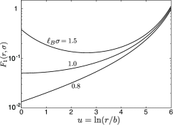
Figure 1: $F_{1}(r,\sigma)=2\pi\ell_{B}r^{2}n_{1}(r)$ vs $\ln(r/b)$ on a logarithmic scale for $\ell_{B}\sigma=0.8,1$, and 1.5 with $M=6$ for one component solvent without salt. The slope of the curve at $r/b=1$ changes its sign at $\ell_{B}\sigma=1$.

In Fig,1, we show $F_{1}(r,\sigma)$ for $\ell_{B}\sigma=0.8,1$, and 1.5 at $M=6$ treating $F_{1}$ as a function of $u\equiv\ln(r/b)$. The area below each curve is the Manning parameter since

$$\int_{0}^{M}duF_{1}(r,\sigma)=\ell_{B}\sigma.$$ (2.19)

We notice that $F_{1}(r,\sigma)$ changes most drastically at $r=b$ and most weakly at $r=R$. Its value at $r=b$ is the normalized counterion density at the rod surface since $F_{1}(b,\sigma)=2\pi\ell_{B}b^{2}n_{1}(b)$. To examine it, we introduce a scaling variable $q$ by

$$q=(\ell_{B}\sigma-1)M.$$ (2.20)

At $\sigma=\sigma^{*}$ we have $q=-M/(1+M)\cong-1$. The relations in Appendix A yield

$$F_{1}(b,\sigma) \cong 2\sigma\ell_{B}(\sigma\ell_{B}-1)^{2}e^{2q}\quad(-q\gg 1),$$ (2.21)

$$\cong (\sigma\ell_{B}-1)^{2}\quad(q\gg 1).$$

For $|q|\sim 1$ we have $F_{1}(b,\sigma)\sim M^{-2}$. Thus $F_{1}(b,\sigma)$ is very small for $-q\gtrsim 1$ with increasing $M$, while it tends to be independent of $M$ for $q\gg 1$.

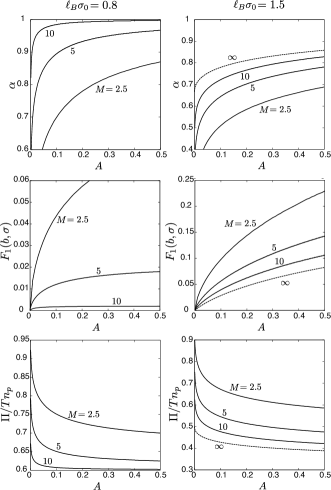
Figure 2: Degree of ionization $\alpha$ (top) , normalized counterion density $F_{1}(b,\sigma)$ on the rod surface (middle), and osmotic pressure $\Pi$ at $r=R$ divided by $Tn_{p}=T\sigma/\pi R^{2}$ (bottom) as functions of $A$ in Eq.(2.22) for $\ell_{B}\sigma_{0}=0.8$ (left) and 1.5 (right) in one component solvent without salt.

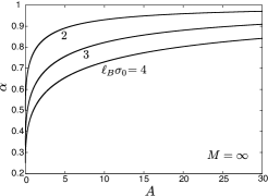
Figure 3: Degree of ionization $\alpha$ vs $A$ for $\ell_{B}\sigma_{0}=2$, 3, and 4 obtained from the asymptotic equation (2.26) in the limit $R\to\infty$ in one component solvent without salt. Here $\alpha\to 1/\ell_{B}\sigma_{0}$ as $A\to 0$, while $\alpha\to 1$ for $A\gg 1$.

We now calculate the degree of ionization $\alpha$ from the mass action law Eq.(2.14). We introduce a normalized dissociation constant,

$$A=2\pi\ell_{B}b^{2}K_{0}.$$ (2.22)

In terms of $A$, Eq.(2.14) is rewritten as

$$\alpha F_{1}(b,\sigma)=(1-\alpha)A.$$ (2.23)

In Fig. 2, we plot numerical results of $\alpha$, $F_{1}(b,\sigma)$, and $\Pi/Tn_{p}$ for $\ell_{B}\sigma_{0}=0.8$ (left) and $1.5$ (right). Here we introduce the osmotic pressure at $r=R$,

$$\Pi=Tn_{1}(R)$$ (2.24)

where the Maxwell stress vanishes from Eq.(2.5). The $n_{p}=\sigma/\pi R^{2}$ is the counterion density for the uniform distribution.

The first line of Eq.(2.21) gives

$$(1-\ell_{B}\sigma_{0}\alpha)^{2}\alpha^{2}/(1-\alpha)\cong{A}(R/b)^{2q}/{2\ell_{B}\sigma_{0}},$$ (2.25)

for $-q=(1-\ell_{B}\sigma)M\gg 1$. The right hand side anomalously depends on $R$ and is very small for $R/b\gg 1$. On the other hand, the second line of Eq.(2.21) gives

$$(\ell_{B}\sigma_{0}\alpha-1)^{2}\alpha\cong A(1-\alpha).$$ (2.26)

for $q=(\ell_{B}\sigma-1)M\gg 1$. This cubic equation of $\alpha$ is the asymptotic equation independent of $R$, yielding a unique solution in the range $(\ell_{B}\sigma_{0})^{-1}<\alpha<1$. Namely, $\alpha\rightarrow(\ell_{B}\sigma_{0})^{-1}<1$ as $A\rightarrow 0$, while $\alpha\rightarrow 1$ with increasing $A$. In Fig. 3, we show this limiting $\alpha$ obtained from Eq.(2.26) as a function of $A$ for $\ell_{B}\sigma_{0}>1$, where the increase of $\alpha$ from 0 to $(\ell_{B}\sigma_{0})^{-1}$ in the narrow region $0<A\lesssim(b/R)^{2}$ is not shown.

II.2.2 Grand potential and effective polymer-solvent interaction

In equilibrium without salt, the grand potential $\Omega$ in Eq.(2.13) consists of three negative parts as

$${\Omega}/{TL}=-2\sigma-\ell_{B}^{-1}{\cal F}_{e}(\ell_{B}\sigma)+\sigma_{0}\ln(1-\alpha),$$ (2.27)

The electrostatic energy $F_{e}=\int d{\mbox{\boldmath$r$}}\varepsilon E^{2}/8\pi$ is equal to $TL(\sigma+\ell_{B}^{-1}{\cal F}_{e})$. See Appendix A for the exact expression for the scaling function ${\cal F}_{e}(s)$, which was derived by Naji and Netz Netz . (i) For small $\ell_{B}\sigma\ll M^{-1}$ the electrostatic part is negligible and ${\Omega}/TL\cong-\sigma+\sigma_{0}\ln(1-\alpha)$. (ii) For $M^{-1}\ll\ell_{B}\sigma\ll 1$ we have

$${F}_{e}\cong TL\ell_{B}\sigma^{2}M,$$

$${\Omega}/TL\cong-\ell_{B}\sigma^{2}M+\sigma_{0}\ln(1-\alpha).$$ (2.28)

(iii) On the other hand, for $\ell_{B}\sigma-1\gg M^{-1}$ and $\ell_{B}\sigma\ll M$, we find

$${F}_{e}\cong TL\ell_{B}^{-1}M,$$

$${\Omega}/TL\cong-\ell_{B}^{-1}M+\sigma_{0}\ln(1-\alpha).$$ (2.29)

Here the electrostatic energy is nearly equal to that of a charged rod at $\sigma=\ell_{B}^{-1}$ without screening. This result suggests that a fraction of $1-(\ell_{B}\sigma)^{-1}$ of the counterions are localized around the rod, as well as the osmotic pressure behavior in Eq.(A4).

Polymer chains in water are often hydrophobic without ionization but can be hydrophilic with ionization Volk ; Rubinstein ; Baigl1 . This means that the polymer-solvent interaction parameter, written as $\chi_{ps}$, is effectively decreased upon ionization. Its decrease $\Delta\chi_{ps}$ may be defined as follows. In the Flory-Huggins free energy density of polymer solutions, the interaction part is written as $Tv_{0}^{-1}\chi_{\rm ps}\phi_{p}$ for small polymer volume fraction $\phi_{p}$, where $v_{0}$ is the solvent volume. We map our polyelectrolytes system to a neutral polymer system. In the present case, the polymer volume is $\pi b^{2}L$ in the total volume $V=\pi LR^{2}$ so that $\phi_{p}=(b/R)^{2}$. We set

$$Tv_{0}^{-1}\Delta\chi_{ps}\phi_{p}=\Omega/V+\Pi.$$ (2.30)

Without salt we have $\Pi=Tn_{1}(R)$ and

$$\Delta\chi_{ps}=\frac{v_{0}}{\pi b^{2}}\bigg{[}\frac{\Omega}{TL}+\pi R^{2}n_{1}(R)\bigg{]}.$$ (2.31)

Here in the brackets, the first term is given by Eq.(2.27) and the second term is equal to $F_{1}(R,\sigma)/{2\ell_{B}}$ from Eq.(2.16). We confirm the negativity of $\Delta\chi_{ps}$ as follows. (i) For small $\ell_{B}\sigma\ll M^{-1}$ we have $\Delta\chi_{ps}\cong(v_{0}/\pi b^{2})\sigma_{0}\ln(1-\alpha)$. (ii) For $M^{-1}\ll\ell_{B}\sigma\ll 1$ we have $\Delta\chi_{ps}\cong(v_{0}/\pi b^{2})[-\ell_{B}\sigma^{2}+\sigma_{0}\ln(1-\alpha)]$. (iii) For $\ell_{B}\sigma-1\gg M^{-1}$ and $\ell_{B}\sigma\ll M$, we have $\Delta\chi_{ps}\cong(v_{0}/\pi b^{2})\Omega/TL$, where $\Omega$ is given by Eq.(2.29).

III Rod in two component solvent

We next consider a charged rod in a nearly incompressible two component solvent such as a mixture of water+alcohol or water+ organic solvent in the same geometry as in the one component case. The volume fraction of the water-like component is $\phi(r)$ and that of the less polar component is $1-\phi(r)$. The molecular volumes of the two components (the inverse densities of the pure components) are assumed to be given by a common volume $v_{0}=a^{3}$, which may be equated with $v_{0}$ in Eq.(2.7). Hence $\phi$ will also be called the composition. We assume small ions and neglect their volume fraction. As in the previous section, $n_{1}(r)$ is the density of the counterions plus the cations of the same species added as a salt.

We suppose a polymer chain with a hydrophobic backbone (like polystyrene) and ionizable groups attached to it Rubinstein . With addition of water, we first need to consider the formation of solvation (or hydration) shells composed of several water molecules around hydrophilic charged particles Is . This can occur even at very small water content Osakai , as will be discussed in Appendix C.

III.1 Ginzburg-Landau theory

For not very small bulk water composition $\phi_{B}$, the water composition $\phi(r)$ varies on mesoscopic scales. To describe such situations, we present a Ginzburg-Landau theory with the gradient free energy of the composition Onukibook .

III.1.1 Free energy including solvation interaction

The total free energy is composed of three parts as $F=F_{0}+F_{d}+\Delta F$, where $F_{0}$ is given in Eq.(2.7) and $F_{d}$ in Eq.(2.8). Notice that $\Delta_{0}$ in Eq.(2.7) should be replaced by $\tilde{\Delta}_{0}$ in Eq.(C7) to account for the solvation shell formation. Hereafter we will redefine $\Delta_{0}$ as the right hand side of Eq.(C7). Then $T\Delta_{0}$ in the following is the renormalized dissociation energy per counterion.

Assuming the homogeneity along the rod, we write the additional contribution $\Delta F$ in the form,

$$\frac{\Delta F}{T} = \int d{\mbox{\boldmath$r$}}\bigg{[}\frac{f_{0}(\phi)}{T}+\frac{C}{2}|\nabla\phi|^{2}-\sum_{i}g_{i}{n_{i}}\phi\bigg{]}$$ (3.1)

$$-2\pi bL\gamma\phi_{s}-L\Delta_{1}\sigma_{0}\alpha\phi_{s}.$$

The space integral is in the cell, $b<r<R$ and $0<z<L$. The free energy density $f_{0}(\phi)$ is taken to be the Bragg-Williams form,

$$f_{0}=\frac{T}{v_{0}}[{\phi}\ln\phi+(1-\phi)\ln(1-\phi)+\chi\phi(1-\phi)],$$ (3.2)

where $\chi$ is the interaction parameter dependent on $T$ and its mean-field critical value is $2$ in the absence of ions. The coefficient $C$ of the gradient part is a positive constant of order $a^{-1}$ and will be taken to be $3a^{-1}$ in our numerical analysis. The coupling terms $(\propto g_{i}$) arise from the ion-dipole interactions among the ions and the polar solvent molecules. In the second line of Eq.(3.1), the term proportional to $\gamma$ arises from the short-range interaction between the rod surface and the solvent molecules Cahn , while the term proportional to $\Delta_{1}$ represents the solvation interaction between the surface charge and the solvent molecules. We neglect the interaction between the mobile ions and the uncharged monomers (which can be important for polar monomers Onuki-Okamoto ). Hereafter,

$$\phi_{s}=\phi(b)$$ (3.3)

is the surface value of the composition (outside the solvation shells under the condition (C8)). These molecular interactions of the rod are characterized by the two constants $\gamma$ and $\Delta_{1}$, which can be either negative or positive.

In $F_{0}$ in Eq.(2.7), the dielectric constant $\varepsilon$ is assumed to depend on the composition in the linear form Debye-Kleboth ,

$$\varepsilon(\phi)=\varepsilon_{0}+\varepsilon_{1}\phi,$$ (3.4)

where $\varepsilon_{0}+\varepsilon_{1}$ is the dielectric constant of the first component and $\varepsilon_{0}$ is that of the second component. Thus $\varepsilon(\phi)$ is inhomogeneous. The electric potential $\Phi(r)$ satisfies

$$\frac{1}{r}\frac{d}{dr}r\varepsilon(\phi)\frac{d}{dr}\Phi=-4\pi\rho,$$ (3.5)

under the boundary conditions $E(R)=0$ and

$$E(b)=-2e\sigma/\varepsilon(\phi_{s})b.$$ (3.6)

III.1.2 Equilibrium and composition-dependent mass action law

We minimize the grand potential $\Omega$ defined as in Eq.(2.9) with $F=F_{0}+F_{d}+\Delta F$. The counterparts of Eqs.(2.11) and (2.12) read

$$\frac{\alpha}{1-\alpha}=\exp\left[\lambda+\frac{e\Phi(b)}{T}-\Delta_{0}+\Delta_{1}\phi_{s}\right],$$ (3.7)

$$n_{i}(r)=n_{0i}\exp\left[-Z_{i}\frac{e\Phi(r)}{T}+g_{i}\phi(r)\right],$$ (3.8)

where $n_{0i}=v_{0}^{-1}e^{\mu_{i}/T-Z_{i}\lambda}$. As in Sec.1, we may set $\lambda=0$ without loss of generality. From these equations the mass action law follows as

$$\frac{\alpha}{1-\alpha}n_{1}(b)=K(\phi_{s}).$$ (3.9)

The dissociation constant $K(\phi_{s})$ depends on the surface composition $\phi_{s}$ as

$$K(\phi_{s})=n_{01}e^{-\Delta_{0}+(\Delta_{1}+g_{1})\phi_{s}}.$$ (3.10)

With increasing $\phi_{s}$, $K(\phi_{s})$ increases (decreases) for positive (negative) $\Delta_{1}+g_{1}$. We are not aware of experimental data on the composition dependence of $\alpha$ for polymers in mixture solvents. On the other hand, strong composition dependence has been reported in dissociation of weak acids in various aqueous mixtures Ohtaki ; Bonn .

The functional derivative $h=\delta F/\delta\phi$ at fixed $n_{i}$ and $\alpha$ is the chemical potential difference of the two components divided by $v_{0}$ and is homogeneous in equilibrium. From Eqs.(2.10) and (3.1) we obtain

$$h=f^{\prime}_{0}(\phi)-TC\nabla^{2}\phi-T\sum_{i}g_{i}n_{i}-\frac{\varepsilon_{1}}{8\pi}E^{2},$$ (3.11)

where $f^{\prime}_{0}(\phi)=\partial f_{0}(\phi)/\partial\phi$ and $E=-d\Phi/dr$. In equilibrium $h$ is a homogeneous constant.

With these results it is convenient to redefine the grand potential for two component solvent as

$$\Omega=F-\int d{\mbox{\boldmath$r$}}\bigg{[}\sum_{i}\mu_{i}n_{i}+f_{0}(\phi_{B})+h(\phi-\phi_{B})\bigg{]},$$ (3.12)

where $\phi_{B}=\phi(R)$ is the value of $\phi$ at $r=R$. As in Eq.(2.13) some calculations give

$$\frac{\Omega}{TL}=2\pi\int_{b}^{R}d{r}r\bigg{[}\frac{1}{T}\hat{f}_{0}(\phi)+\frac{C}{2}\phi^{\prime 2}\bigg{]}-2\pi b\gamma\phi_{s}$$

$$\hskip 14.22636pt-\sigma+\sigma_{0}\ln(1-\alpha)-\frac{F_{e}}{TL}-\frac{N_{\rm s}}{L}.$$ (3.13)

In the first line we write $\phi^{\prime}=d\phi/dr$ and define

$$\hat{f}_{0}(\phi)=f_{0}(\phi)-f_{0}(\phi_{B})-h(\phi-\phi_{B}).$$ (3.14)

The first line of Eq.(3.13) gives the compositional contribution. The second line is of the same form as the right hand side of Eq.(2.14) with $N_{s}$ being the number of ions added as salt.

Small variations of $\phi$, $\alpha$, and $n_{i}$ yield an incremental change of $\Omega$, written as $\delta\Omega$. With the equilibrium conditions (3.5), (3.7), (3.8), and (3.11), its linear terms proportional to $\delta\alpha$ and $\delta n_{i}$ vanish. There remain surface parts of the form,

$$\frac{\delta\Omega}{LT} = 2\pi C[(r\phi^{\prime}\delta\phi)_{r=R}-(r\phi^{\prime}\delta\phi)_{r=b}]$$ (3.15)

$$-(2\pi b\gamma+\Delta_{1}\sigma)\delta\phi(b).$$

We set $\delta\Omega=0$ for any boundary variations $\delta\phi(b)$ and $\delta\phi(R)$ to obtain

$$\phi^{\prime}(R)=0,$$ (3.16)

$$C\phi^{\prime}(b)=-\gamma-(\Delta_{1}/2\pi b)\sigma,$$ (3.17)

which are the boundary conditions on $\phi$ in solving the equation $h=$const. in Eq.(3.11). In our theory the condition at $r=b$ in Eq.(3.17) depends on $\sigma$. For positive (negative) $\gamma+\Delta_{1}\sigma/2\pi b$, the first component tends to be attracted to (repelled from) the rod. A similar boundary condition has been used in the gradient theory of the wetting transition on a planar wall Cahn .

We use the gradient free energy. It is usually derived from the gradient expansion of the two body van der Waals interactions and is justified near the critical point. In the following, however, we will present numerical results in the composition range $0.15<\phi_{B}<0.53$, imposing the boundary condition (3.17) in the gradient theory, where $\phi_{B}$ is the composition far from the rod. When the rod radius $b$ is of order $a$ and $\phi$ changes steeply around the rod, a density functional theory without the gradient expansion should yield more reliable results Ebner ; Evans .

III.1.3 Solvation interaction

In the original Born theory Born , the solvation chemical potential was given by $\mu_{\rm sol}^{i}(\phi)=Z_{i}^{2}e^{2}/2\varepsilon(\phi)R_{i}$ for ion species $i$, where $Z_{i}e$ is the charge, $\varepsilon(\phi)$ is the solvent dielectric constant dependent on $\phi$, and $R_{i}$ is a microscopic length called the Born radius. However, this formula is a crude approximation and is not applicable to hydrophobic ions. In this paper we assume the form

$$\mu_{\rm sol}^{i}(\phi)=\mu_{\rm sol}^{i}(0)-Tg_{i}\phi.$$ (3.18)

The solvation contribution to the free energy density is given by $\sum_{i}\mu_{\rm sol}^{i}(\phi)n_{i}$, yielding the terms proportional to $g_{i}$ on the right hand side of Eq.(3.1). For a mixture of water and oil, for example, $Tg_{i}$ is the difference of the solvation chemical potential in oil and that in water. Therefore, $g_{i}>0$ for hydrophilic ions and $g_{i}<0$ for hydrophobic ions in aqueous mixture solvents.

The difference of $\mu_{\rm sol}^{i}$ between the coexisting phases coincides with the Gibbs transfer energy $\Delta G_{\rm tr}^{i}$ (per ion) in electrochemistry Osakai ; Hung . It becomes $Tg_{i}$ in strong segregation in our theory. Data of $\Delta G_{\rm tr}^{i}$ for water+nitrobenzene at $T\sim 300$K suggest $g_{i}\sim 15$ for monovalent ions such as Na⁺ and $g_{i}\sim-15$ for tetrarphenylborate BPh${}_{4}^{-}$. For water+alcohol, $|g_{i}|$ should not be smaller, since the dielectric constant of nitrobenzene is 35 and that of alcohol is smaller (24 for ethanol). The solvation coupling is thus very strong in aqueous mixtures.

III.1.4 Analysis of behavior of composition deviation

The composition $\phi(r)$ tends to a constant $\phi_{B}$ far from the rod. We treat $\phi_{B}$ as a control parameter. With a salt added, this behavior is obvious if the Debye length $k_{D}^{-1}$ is shorter than the system radius $R$ and longer than the correlation length $\xi$ of the composition. In such a case Eq.(3.11) gives $\phi(r)-\phi_{B}\propto e^{-k_{D}r}$ far from the rod.

Without salt, however, the decay is algebraic. To show it, we linearize Eq.(3.11) with respect to the composition deviation $\delta\phi=\phi-\phi_{B}$ to obtain

$$(1-\xi^{2}\nabla^{2})\delta\phi=\chi_{s}g_{1}n_{1}+\frac{\chi_{s}\varepsilon_{1}}{8\pi T}E^{2},$$ (3.19)

where we assume $|\delta\phi|\ll\phi_{B}$ at any $r$. We define the correlation length $\xi$ and the susceptibility $\chi_{s}$ as

$$\xi = [TC/f^{\prime\prime}_{0}(\phi_{B})]^{1/2},$$ (3.20)

$$\chi_{s} = T/f^{\prime\prime}_{0}(\phi_{B})=\xi^{2}/C,$$ (3.21)

where $f^{\prime\prime}_{0}(\phi)=T[1/\phi(1-\phi)-2\chi]/v_{0}$ from Eq.(3.11). In this paper, we set $C=3/a$; then, $\chi_{s}\sim a\xi^{2}$. The length $\xi$ remains of order $a$ away from the criticality, while it grows near the criticality.

The two terms on the right hand side of Eq.(3.19) roughly behave as $r^{-2}$ from the results for one component solvent. That is, if $F_{1}=2\pi\ell_{B0}r^{2}n_{1}(r)$ in Eq.(2.16) (or in Eq.(3.29) below) is of order unity, the two terms are of order $\chi_{s}g_{1}/2\pi\ell_{Bb}r^{2}$ and $\chi_{s}\varepsilon_{1}/2\pi\varepsilon_{0}\ell_{Bb}r^{2}$, respectively. We define two Bjerrum lengths as

$$\ell_{B0}=e^{2}/\varepsilon_{0}T,\quad\ell_{Bb}=e^{2}/\varepsilon_{B}T,$$ (3.22)

at $\varepsilon=\varepsilon_{0}$ and $\varepsilon=\varepsilon(\phi_{B})=\varepsilon_{B}$, respectively. Thus $\ell_{Bb}=\ell_{B0}/(1+\varepsilon_{1}\phi_{B}/\varepsilon_{0})$. Furthermore, we are interested in the strong solvation case $g_{1}\gg 1$ with $\varepsilon_{1}/\varepsilon_{0}\sim 1$, where the first term dominates over the second in the right hand side of Eq.(3.19). Then $\delta\phi(r)$ decays for $r-b\gtrsim\xi$ as

$$\delta\phi(r)\sim(g_{1}a\xi^{2}/2\pi\ell_{Bb})r^{-2}.$$ (3.23)

Here we are assuming $|\delta\phi|\lesssim\phi_{B}$, which holds even for $r\sim\xi$ if $g_{1}a/2\pi\ell_{Bb}\lesssim 1$.

III.1.5 Effective charge density and modified Manning law

For large $r$ far from the rod, $\phi(r)$ tends to a constant $\phi_{B}$ and $n_{1}(r)$ obeys the nonlinear Poisson-Boltzmann equation even in the salt-free case. We introduce a characteristic length $r_{c}$ in the range $b<r_{c}\ll R$. For $r$ larger than $r_{c}$, we may set $\varepsilon(\phi)\cong\varepsilon_{B}$ with $\varepsilon_{B}=\varepsilon(\phi_{B})$ and the potential $\Phi(r)$ obeys

$$-\varepsilon_{B}\nabla^{2}\Phi\cong 4\pi en_{0}\exp(-e\Phi/T),$$ (3.24)

where we set $Z_{1}=1$ and $n_{0}=n_{01}e^{-\lambda}$. We compare $\Phi(r)$ and $n_{1}(r)$ in our system approximately obeying Eq.(3.24) far from the rod and those obtained as the solution of the nonlinear Poisson-Boltzmann equation,

$$-\varepsilon_{B}\nabla^{2}\Phi_{\rm PB}=4\pi en_{1}^{\rm PB},$$ (3.25)

where $n_{1}^{\rm PB}(r)=n_{0}\exp(-e\Phi_{\rm PB}(r)/T)$ is the corresponding counterion density. We set $\Phi_{\rm PB}^{\prime}(R)=0$ at $r=R$ and impose the boundary condition at $r=r_{c}$ as

$$\Phi_{\rm PB}^{\prime}(r_{c})=\Phi^{\prime}(r_{c}),$$ (3.26)

where $\Phi_{\rm PB}^{\prime}(r)=d\Phi_{\rm PB}(r)/dr$ and $\Phi^{\prime}(r)=d\Phi(r)/dr$. From Eq.(3.25) $\Phi(r)\cong\Phi_{\rm PB}(r)$ and $n_{1}(r)\cong n_{1}^{\rm PB}(r)$ far from the rod $r>r_{c}$, but significant differences can arise in the region $r<r_{c}$.

In terms of $\Phi_{\rm PB}$ we define the effective charge density $\sigma_{\rm eff}$ on the rod by

$$\sigma_{\rm{eff}}=\varepsilon_{B}b\Phi_{\rm PB}^{\prime}(b)/2e.$$ (3.27)

From Eq.(2.6) the real charge density $\sigma$ is given by $\sigma=\varepsilon(\phi_{s})b\Phi^{\prime}(b)/2e$. From Eqs.(3.5), (3.24), and (3.25) the apparent excess charge density $\Delta\sigma=\sigma-\sigma_{\rm{eff}}$ on the rod is expressed as

$$\Delta\sigma = 2\pi n_{0}\int_{b}^{r_{c}}drr[e^{-e\Phi(r)/T}-e^{-e\Phi_{\rm PB}(r)/T}]$$ (3.28)

$$= \frac{1}{\ell_{B0}}\int_{0}^{u_{c}}du[F_{1}(u)-F_{1}^{\rm PB}(u)].$$

In the second line, we set $u=\ln(r/b)$ with $u_{c}=\ln(r_{c}/b)$ being the upper bound and define

$$F_{1}=2\pi r^{2}\ell_{B0}n_{1},$$

$$F_{1}^{\rm PB}=2\pi r^{2}\ell_{B0}n_{1}^{\rm PB},$$ (3.29)

as in Eq.(2.16). These quantities are functions of $u$. In the bottom plates of Fig.4, we shall see that $u_{c}$ may be pushed to infinity since the integrand in the second line of Eq.(3.28) vanishes for large $u$. Here the effective Manning parameter is $\sigma_{\mathrm{eff}}\ell_{Bb}$, where $\ell_{Bb}$ is defined in Eq.(3.22). In terms of $n_{p}^{\mathrm{eff}}\equiv\sigma_{\mathrm{eff}}/\pi R^{2}$ the asymptotic law for the osmotic pressure $\Pi$ in Eq.(A4) is changed to

$${\Pi} \cong Tn_{p}^{\mathrm{eff}}(1-\ell_{Bb}\sigma_{\mathrm{eff}}/2)\quad(\ell_{Bb}\sigma_{\mathrm{eff}}<1)$$ (3.30)

$$\cong Tn_{p}^{\mathrm{eff}}/2\ell_{Bb}\sigma_{\mathrm{eff}}\qquad(\ell_{Bb}\sigma_{\mathrm{eff}}>1).$$

III.1.6 Strong deformations of the counterion distribution

We examine the conditions of strong attraction of the counterions due to a composition change around the rod. We assume that $\phi_{B}$ is not very small and $\xi$ is not much separated from $a$ for simplicity. If $g_{1}\gg 1$, $\delta\phi$ is of order $g_{1}a/2\pi\ell_{Bb}$ at $r\sim\xi$ from Eq.(3.23). Since $n_{1}\propto e^{g_{1}\phi}$ from Eq.(3.8), an appreciable attraction of the counterions is induced due to the composition change when

$$g_{1}^{2}a/2\pi\ell_{Bb}\gtrsim 1.$$ (3.31)

For large $g_{1}\gg 1$ the above condition can be realized while $\delta\phi$ remains small $(\ll\phi_{B}$).

Also $\phi^{\prime}(b)$ satisfies the boundary condition (3.17). This yields a contribution to $\delta\phi(r)$, written as $(\delta\phi)_{b}(r)$. It obeys $(1-\xi^{2}\nabla^{2})(\delta\phi)_{b}=0$ in the bulk, so it decays rapidly far from the rod. If $\xi\lesssim b$, it is approximately written as

$$(\delta\phi)_{b}(r)\cong\bigg{[}\gamma+\frac{\Delta_{1}\sigma}{2\pi b}\bigg{]}\frac{\xi}{C}\exp\bigg{[}-\frac{r-b}{\xi}\bigg{]}.$$ (3.32)

If the above composition change is positive, the counterions are significantly attracted to the rod when

$$g_{1}(\gamma+{\Delta_{1}\sigma}/{2\pi b}){\xi}/{C}\gtrsim 1.$$ (3.33)

If it is negative and its absolute value exceeds unity and if the condition (3.31) does not hold, the counterions should be repelled from the rod.

The criterions (3.31) and (3.33) are crude ones based on many assumptions. In particular, $F_{1}(b)\sim 1$ has been assumed in deriving Eq.(3.31) and the unknown $\sigma=\sigma_{0}\alpha$ is contained in Eq.(3.33). Setting up general criterions is at present difficult, because many of the parameters strongly affect the counterion distribution. Nevertheless, we recognize that the counterion distribution can be changed dramatically even for a slight change of the composition in the strong solvation condition $|g_{1}|\gg 1$.

III.2 Numerical results for two component solvent without salt

We present some numerical results for a water-oil solvent without salt. In all the examples to follow, we numerically solve Eqs.(3.5), (3.7), (3.8), and (3.11) under given boundary conditions by setting

$$b=2a,~{}R/b=e^{6}\cong 403,$$

$$\sigma_{0}=\pi/2a,~{}C=3/a,~{}\Delta_{1}=7,$$

$${\varepsilon_{1}}=2{\varepsilon_{0}},~{}\ell_{B0}=12a/\pi=6/\sigma_{0},$$

where $\ell_{B0}$ is defined in Eq.(3.22). The solvation parameter $g_{1}$ will be either of 5, 7, or 10. Note that $g_{1}$ can be larger in real situations, as discussed below Eq.(3.18). The parameter $A=2\pi\ell_{B0}b^{2}K_{0}$ in Eq.(2.22) will be chosen to be small. As a result, little ionization occurs without composition variations near the rod. In our simulation the counterion density far from the rod is so small such that the solvent phase diagram is unchanged OnukiPRE .

III.2.1 Attraction of water and counterions to a hydrophobic rod

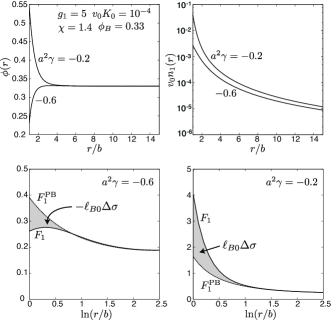
Figure 4: Numerical results for a mixture solvent in the salt-free case for $\chi=1.4$, $\phi_{B}=1/3$, $g_{1}=5$, and $A=0.0096$ (on the point $(+)$ in Fig.6). Top plates: composition $\phi(r)$ (left) and normalized counterion density $v_{0}n_{1}(r)$ (right) for $a^{2}\gamma=-0.6$ and $-0.2$. Bottom plates: $F_{1}(u)$ and $F_{1}^{\rm PB}(u)$ in Eq.(3.29) vs $u=\ln(r/b)$ for $a^{2}\gamma=-0.6$ (right) and $-0.2$ (left). The area between these two functions (shaded) is equal to the normalized excess charge density $\ell_{B0}\Delta\sigma$ from Eq.(3.28).

The interaction between the solvent and the rod in Eq.(3.1) leads to the boundary condition (3.17) in our gradient theory. For $\gamma<0$ ($\gamma>0$), the rod repels (attracts) the water component and is hydrophobic (hydrophilic) without ionization. Even for $\gamma<0$, however, the right hand side of Eq.(3.17) changes from positive to negative with increasing the degree of ionization $\alpha$ and the condition (3.33) can eventually hold for $|\gamma|<\Delta_{1}\sigma/2\pi b$. Then the rod becomes effectively hydrophilic. To examine the resultant preferential adsorption of the water-like component, we introduce

$$\Gamma={2\pi}\int_{b}^{R}drr[\phi(r)-\phi_{B}],$$ (3.34)

where $\phi_{B}$ is the value of $\phi(r)$ at $r=R$.

Figure 4 illustrates such a changeover in the one phase region for (a) $a^{2}\gamma=-0.6$ and (b) $a^{2}\gamma=-0.2$. We set $\chi=1.4$, $\phi_{B}=1/3$, $g_{1}=5$, and $v_{0}K_{0}=10^{-4}$. Then $A=2\pi\ell_{B0}b^{2}K_{0}=0.0096$ from Eq.(2.22), $\xi=1.32a$ from Eq.(3.20), and $v_{0}K=10^{-4}e^{12\phi_{s}}$ from Eq.(3.10). In the upper left panel of Fig.4, we present the composition profile $\phi(r)$ near the rod, which is repelled for (a) and attracted for (b). However, as shown in Eq.(3.23), $\delta\phi=\phi-\phi_{B}$ has a positive tail ($r^{-2}$) without salt, giving rise to a positive logarithmic contribution $\sim(g_{1}a\xi^{2}/\ell_{B0})\ln(R/\xi)$ to the integral $\Gamma$ in Eq.(3.34). Due to this singular contribution we obtain $\Gamma=0.706a^{2}$ for (a), while $\Gamma=3.99a^{2}$ for (b). In the upper right panel, the difference of $n_{1}(r)$ between the two cases is large and $n_{1}(r)$ is written on a semi-logarithmic scale. Here, $\alpha=0.369$, $\phi(b)-\phi_{B}=-0.101$, and $v_{0}n_{1}(b)=2.73\times 10^{-3}$ for (a), while $\alpha=0.621$, $\phi(b)-\phi_{B}=0.214$, $v_{0}n_{1}(b)=4.19\times 10^{-2}$ for (b). The lower panels of Fig.4 display the two functions $F_{1}(u)$ and $F_{1}^{\rm PB}(u)$ in Eq.(3.29) for the two cases. The excess charge density in Eq.(3.28) is negative as $\Delta\sigma=-0.02/\ell_{Bb}=-0.03/\ell_{B0}$ for (a), but is positive as $\Delta\sigma=0.33/\ell_{Bb}=0.56/\ell_{B0}$ for (b).

We then check the criterions (3.31) and (3.33). The left hand side of Eq.(3.31) is 1.73, while that of Eq.(3.33) is $-0.609$ for (a) and $0.755$ for (b). However, $F_{1}(b)=0.109$ for (a) and $1.54$ for (b), so the criterion (3.31) is not justified for (a) (see the discussion above Eq.(3.22)).

III.2.2 First order phase transition of ionization without salt

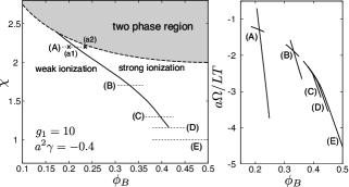
Figure 5: Right: Phase diagram in the $\phi_{B}$-$\chi$ plane, where $g_{1}=10$, $K_{0}v_{0}=8\times 10^{-6}$, and $a^{2}\gamma=-0.4$ for water-oil solvent without salt. Left: Normalized grand potential $a\Omega/LT$ on lines (A)-(E). For (A)-(C) there are two branches of weak and strong ionization and the equilibrium is given by the lower branch, while for (D) and (E) there is only one branch.

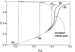
Figure 6: Degree of ionization $\alpha$ vs $\phi_{B}$ without salt along the lines (A)$\sim$(E) in Fig.5, where $g_{1}=10$, $K_{0}v_{0}=8\times 10^{-6}$, and $a^{2}\gamma=-0.4$. The discontinuity (broken line segments) vanishes at the critical point of ionization.

With increasing $\phi_{B}$ we predict a first order phase transition from weak to strong ionization. We suppose that the backbone is hydrophobic, the ionization is weak in the pure second component, and the counterions are strongly hydrophilic. Hence, in Figs. 5-9, we set $a^{2}\gamma=-0.4\times 10^{-6}$, $v_{0}K_{0}=8$, and $g_{1}=10$.

We vary $\phi_{B}$ at fixed $\chi$ on the lines (A)-(E) in the left panel of Fig.5, where $\chi=2.2$ (A), 1.7 (B), 1.3 (C), 1.16 (D), and 1 (E). For $\chi>\chi^{\rm cri}$, there are two branches of weak and strong ionization around a first order transition line expressed as

$$\phi_{B}=\phi_{B}^{\rm tra}(\chi).$$ (3.35)

It starts from a point given by $(\phi_{B},\chi)=(0.1736,2.39)$ on the solvent coexistence curve and ends at a critical point given by $(\phi_{B},\chi)=(\phi_{B}^{\rm cri},\chi^{\rm cri})=(0.415,1.16)$, where $\phi_{B}^{\rm cri}=\phi_{B}^{\rm tra}(\chi^{\rm cri})$. In the right panel of Fig.5, the grand potential $\Omega$ in Eq.(3.13) is calculated, which is lower on the equilibrium branch than on the metastable one. In Fig. 6, we show $\alpha$ vs $\phi_{B}$ on the lines (A)-(E), where (A)-(C) pass through the transition line, (D) passes through the critical point, and (E) is a supercritical path. This ionization transition is analogous to the prewetting phase transition on a wall Cahn ; Ebner ; Evans , where a first order phase transition line also starts from the coexistence curve ending at a critical point.

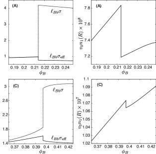
Figure 7: Charge density $\sigma$ and effective charge density $\sigma_{\rm eff}$ in Eq.(3.19) on the rod around the transition in units of $\ell_{Bb}^{-1}$ (left). Counterion density $n_{1}(R)=\Pi/T$ on the outer surface in units of $v_{0}^{-1}$ (right). These are plotted as functions of $\phi_{B}$ on the line (A) (upper plates) and on the line (C) (lower plates) in Fig.5. In the weakly ionized phase, $\ell_{Bb}\sigma$ is smaller than unity for (A) and larger than unity for (C), leading to larger discontinuities for (A) than for (C).

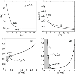
Figure 8: Profiles without salt at the two points (a1) (weakly ionized state) and (a2) (strongly ionized state) on the line (A) in Fig.5. Top plates: $\phi(r)$ (left) and $v_{0}n_{1}(r)$ (right) vs $r/b$. Bottom plates: $F_{1}$ and $F_{1}^{\rm{PB}}$ vs $\ln(r/b)$ for (a1)(left) and (a2)(right). From Eq.(3.28) the area of the gray region is equal to $-\ell_{B0}\Delta\sigma$ for (a1) and to $\ell_{B0}\Delta\sigma$ for (a2).

In the left panels of Fig.7, we show the charge densities $\sigma$ and $\sigma_{\rm eff}$ multiplied by $\ell_{Bb}$ on the lines (A) and (C), where $\ell_{Bb}$ is defined in Eq.(3.22) and $\sigma_{\rm eff}$ by Eq.(3.27). In these cases, $\ell_{Bb}\sigma$ increases but $\ell_{Bb}\sigma_{\rm eff}$ decreases at the transition from weak to strong ionization, The counterions are more strongly attracted to the rod in the strongly ionized state than in the weakly ionized state (see Fig.8 below). The right panels of Fig.7 display the counterion density $n_{1}(R)=\Pi/T$ on the outer surface as a function of $\phi_{B}$. Counter-intuitively, $\Pi$ decreases discontinuously at the transition with increasing $\alpha$. The jump of $\Pi$ at the transition is of order $8\%$ on the line (A) and $1\%$ on the line (C) in accord with the modified Manning limiting law (3.30). Here the effective Manning parameter $\ell_{Bb}\sigma_{\mathrm{eff}}$ is smaller than unity on the line (A) and larger than unity on the line (C).

In Fig.8, we show the spatial profiles of $\phi(r)$, $n_{1}(r)$, $F_{1}(r)$, and $F_{1}^{\rm{PB}}(r)$ at the two points (a1) and (a2) on the line (A) in Fig.5. The left hand sides of Eqs.(3.31) and (3.33) are equal to $5.83$ and $-0.877$ for (a1) and to $6.13$ and $2.53$ for (a2), respectively. Here, $\alpha=0.221$, $\phi_{b}=0.143$, $v_{0}n_{1}(b)=3.20\times 10^{-4}$, and $\Gamma=0.706a^{2}$ at (a1), while $\alpha=0.998$, $\phi_{b}=0.982$, $v_{0}n_{1}(b)=0.245$, and $\Gamma=3.99a^{2}$ at (a2). The upper left panel of Fig.8 shows that the water component is considerably depleted from the rod at (a1) but it covers the rod almost completely at (a2). The upper right panel of Fig.8 indicates that the counterions are more accumulated around the rod at (a2) than at (a1) such that they are more depleted far from the rod at (a2) than at (a1). In the lower panels of Fig.8 the excess charge density $\Delta\sigma$ in Eq.(3.28) is $-0.003/\ell_{Bb}$ at (a1) and $3.32/\ell_{Bb}$ at (a2).

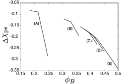
Figure 9: Change of the effective polymer-solvent interaction parameter $\Delta\chi_{ps}$ due to ionization for a two component solvent without salt along the paths (A)-(E) in Fig.5.

In Fig.9, we plot the change of the effective polymer-solvent interaction parameter $\Delta\chi_{ps}$ in Eq.(2.31) along the paths (A)-(E). Its negativity indicates that the solvent quality becomes effectively better with ionization and adsorption. In the brackets of Eq.(2.31), the second term $\pi R^{2}n(R)$ is at most 10$\%$ of the first term $\Omega/TL$ and its discontinuity at the transition is very small.

We comment on the grand potential $\Omega$ in Eq.(3.13). At the transition, the composition part (the first line) increases due to the layer formation, while the dissociation part (the first two terms in the second line) decreases. The change of the electrostatic part is much smaller than these changes in the present case. At the transition point on the line A, these three parts (multiplied by $a$) are given by $(0.848,-0.775,-1.36)$ and $(11.0,-11.0,-1.28)$ in the weakly and strongly ionized states, respectively.

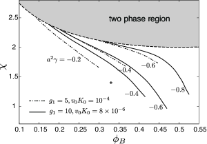
Figure 10: First-order phase transition lines of ionization in the $\phi_{B}$-$\chi$ plane for various parameter values without salt. Solid lines: $a^{2}\gamma=-0.4,-0.6,$ and $-0.8$ with $g_{1}=7$ and $K_{0}v_{0}=8\times 10^{-6}$. Broken lines: $a^{2}\gamma=-0.2,-0.4,$ and $-0.6$ with $g_{1}=5$ and $K_{0}v_{0}=10^{-4}$. Each line starts from a point on the solvent coexistence curve and ends at a critical point with decreasing $\chi$ in the bulk one-phase region.

The first order phase transition can occur over a wide range of the parameters both without and with salt. In Fig.10, the first order phase transition lines are displayed for various $g_{1}$ and $\gamma$ without salt, which start from the solvent coexistence curve to end at an ionization critical point. These lines are markedly enlarged with increasing the hydrophilic solvation strength $(g_{1}>0)$ and/or the rod hydrophobicity $(\gamma<0)$. The transition with salt will be examined in future.

III.2.3 Profiles near the solvent coexistence curve without salt

In the following we examine the profiles of $\phi(r)$ and $n_{1}(r)$ close to the water-poor branch of the solvent coexistence curve ($\phi_{B}\leq 1/2$). We vary $\phi_{B}$ and $\chi$ fixing the other parameters as in Figs.5-9. Namely, $g_{1}=10$, $a^{2}\gamma=-0.4$, and $v_{0}K_{0}=8\times 10^{-6}$.

Figure 11 presents the profiles at two points, $(\phi_{B},\chi)=(0.1730,2.392)$ and $(0.1740,2.389)$, between the transition point $(\phi_{B},\chi)=(0.1736,2.390)$ on the coexistence curve. We recognize marked jumps at the transition. That is, at the weakly ionized state at $\phi_{B}=0.173$, we have $\alpha=0.202$, $\sigma=1.21\ell_{B0}^{-1}=0.900\ell_{Bb}^{-1}$, and $\Gamma=0.565a^{2}$, while at the strongly ionized state at $\phi_{B}=0.174$, we have $\alpha=0.999$, $\sigma=5.99\ell_{B0}^{-1}=4.44\ell_{Bb}^{-1}$, and $\Gamma=27.2a^{2}$. The first component remains repelled around the rod in the weakly ionized phase but is much attracted around it in the strongly ionized phase.

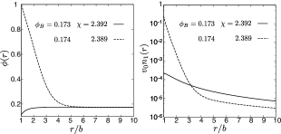
Figure 11: Composition $\phi(r)$ and normalized counterion density $v_{0}n_{1}(r)$ on the coexistence curve for $(\phi_{B},\chi)=(0.1730,2.392)$ in the weakly ionized phase (bold lines) and $(0.1740,2.389)$ in the strongly ionized phase (dotted lines). The line of the first order ionization phase transition starts between these two points as in the right panel of Fig.5.

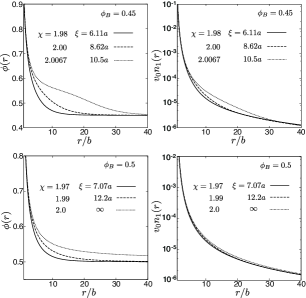
Figure 12: Composition $\phi(r)$ and normalized counterion density $v_{0}n_{1}(r)$ near the solvent coexistence curve for $0.45$ (top), and $0.5$ (bottom). Values of $\chi$ and $\xi$ are given within each panel.

In the upper panels of Fig.12, we set $\phi_{B}=0.45$ to obtain $\Gamma/a^{2}=86.6$, $178$, and $497$ for $\chi=1.9,2.0$, and $2.0067$, respectively. The point $(\phi_{B},\chi)=(0.45,2.0067)$ is on the coexistence curve. In the lower panels, we set $\phi_{B}=0.5$ to obtain $\Gamma/a^{2}=88.9,211.0,$ and $8691$ for $\chi=1.97,1.990$, and $2.0$, respectively. A shoulder in $\phi(r)$ at $(\phi_{B},\chi)=(0.45,2.03)$ (left in the top) represents a water-rich layer varying gradually. At the solvent critical point, the excess deviation $\delta\phi(r)=\phi(r)-\phi_{B}$ decays as $\delta\phi(r)\sim r^{-1}$ for $r/a\lesssim 10$ and $\delta\phi(r)\sim r^{-2}$ for $10\lesssim r/a\lesssim 50$. In all these cases, the dissociation is nearly complete or $\alpha\cong 1$.

Marcus et al. Tsori1 obtained a water-rich layer separated from the water-poor bulk region by a sharp boundary around a rod or a sphere. In our scheme, a layer with an interface follows in the low density limit of the counterions (realized for very large $R$) and under the conditions $\gamma=\Delta_{1}=0$ (which yields the boundary condition $\phi^{\prime}(b)=0$ from Eq.(3.17)). In addition, if the bulk region is metastable (inside the solvent coexistence curve), a layer around a chain can trigger phase separation. This is analogous to the nucleation process around a charged particle in metastable polar fluids Kitamura .

IV Summary and Remarks

In this paper, the ion distributions have been examined around a charged rod when the degree of ionization $\alpha$ is a fluctuating quantity. In mixture solvents, the effect of the preferential solvation has been investigated.

In Sec.II, a long ionizable rod in a one component solvent has been treated, where the dissociation process gives rise to the free energy contribution $F_{d}$ in Eq.(2.8). Minimization of the grand potential $\Omega$ in Eq.(2.9) has then yielded $\alpha$ obeying the mass action law and the charge distribution $n_{1}(r)$ obeying the Poisson-Boltzmann equation. In Subsec.IIB, we have examined the counterion density at the rod surface without salt on the basis of the exact results Fuoss . For considerably large $M=\ln(R/b)$, $\alpha$ is determined by Eq.(2.25) for $(1-\sigma\ell_{B})M\gg 1$ and by Eq.(2.26) for $(\sigma\ell_{B}-1)M\gg 1$. All the quantities sensitively depend on the parameter $A(\propto K_{0})$ in Eq.(2.22) as in Fig.2. In the limit $M\gg 1$, $\alpha$ tends to unity in the former and to a well-defined limit in the range $(\ell_{B}\sigma_{0})^{-1}<\alpha<1$ in the latter as in Fig.3.

In Subsec.IIIA, we have generalized our theory in Sec.II to describe the ionization equilibrium in mixture solvents. The additional free energy is $\Delta F$ in Eq.(3.1) for the composition $\phi$, which includes the solvation couplings with ions ($\propto g_{i}$) and the ionized monomers ($\propto\Delta_{1}$). The Manning limiting law for the osmotic pressure (A4) is modified to Eq. (3.30). Though still fragmentary, Subsec.IIIB has presented numerical results without salt, where the solvent consists of a water-like component and a less polar component. The counterions and the charged monomers are hydrophilic with $g_{1}>0$ and $\Delta_{1}>0$. Even if a rod is hydrophobic with $\gamma<0$, it becomes effectively hydrophilic with ionization as in Fig.4. We have found a first order phase transition of ionization for hydrophilic counterions around a hydrophobic rod as in Figs.5-8. At the transition from weakly to strongly ionized states, the number of the counterions increases, but the osmotic pressure has decreased in our examples as in Fig.7. The polymer-solvent interaction parameter $\chi_{ps}$ decreases upon ionization as in Fig.9. We have examined the composition and counterion profiles at the crosspoint of the ionization transition line and the coexistence curve in Fig.11 and near the coexistence curve in the strongly ionized phase in Fig.12. The adsorption $\Gamma$ of the composition in Eq.(3.34) much increases near the coexistence curve in the strongly ionized phase. The adsorption is long-ranged near the solvent criticality. In Appendix B, we will add a salt, where $\alpha$ is a decreasing function of the salt density. In Appendix C, we will examine the solvation shell formation at small content of a polar solute.

We make further remarks on the first order phase transition of ionization of an ionizable rod. Here we suppose that a polymer chain can be in an expanded coil state in a weakly ionized state and in a more expanded state after the transition without coil-globule transition. We have calculated inhomogeneities perpendicular to the chain, but those along the chain should also be important and can well alter the nature of the transition.

Finally, we mention previous and proposed experiments. (i) Many authors have studied the conformation of a neutral polymer near the solvent critical point Brochard ; mixture ; Sumi . The effect of the critical fluctuations is much more enhanced on a charged polymer in a polar binary mixture. (ii) In near-critical binary mixtures with salt Anisimov and in polyelectrolytes Ise ; Kuil ; Amis , ion-induced aggregates have been observed, where relevance should be the preferential solvation. (iii) We may replace hydrophilic counterions by hydrophobic ions Osakai ; Hung such as tetrarphenylborate BPh${}_{4}^{-}$. For hydrophilic and hydrophobic ion pairs, the preferential solvation can be much stronger than for hydrophilic ion pairs OnukiJCP . Sadakane et al. Sadakane added NaBPh₄ into a binary mixture to obtain mesophases. (iv) Ionic surfactants can be adsorbed to DNA even if their bulk concentration is very small Yoshi1 ; Shirahama . The resultant complex can be solubilized in organic solvents such as ethanol cationic . Kuhn et al. predicted that this adsorption can occur as a first order phase transition Levin1 .

In future work, we will treat two parallel rods in mixture solvent, between which there can arise attraction mediated by the composition fluctuations.

$$\frac{F_{1}(r,\sigma)}{B^{2}}=[\sinh(B\ln\hat{r}-\tanh^{-1}B)]^{-2}\quad(\sigma<\sigma^{*})$$

$$=[\sin(B\ln\hat{r}-\tan^{-1}B)]^{-2}\quad(\sigma>\sigma^{*}).$$ (A1)

The parameter $B$ is the solution of the equation,

$$\frac{1-\ell_{B}\sigma}{B}=\coth[BM+\tanh^{-1}B]\quad(\sigma<\sigma^{*})$$

$$\hskip 12.80365pt=\cot[BM+\tan^{-1}B]\quad(\sigma>\sigma^{*}),$$ (A2)

where we may set $B\geq 0$. At $\sigma=\sigma^{*}$, we have $B=0$ and $F_{1}(r,\sigma^{*})=(1-\ln\hat{r})^{-2}$ for any $M>0$. At $r=b$ it holds

$$F_{1}(b,\sigma)=(\ell_{B}\sigma-1)^{2}\mp B^{2},$$ (A3)

where $-$ is for $\sigma<\sigma^{*}$ and $+$ is for $\sigma>\sigma^{*}$ in the right hand side. For $M\gg 1$ we find $B\cong 1-\ell_{B}\sigma$ for $-q\gg 1$ and $B\cong\pi/M$ for $q\gg 1$ in terms of $q$ in Eq.(2.20).

At $r=R$ we obtain the large $M$ behavior $F_{1}(R,\sigma)\cong 1-(1-\ell_{B}\sigma)^{2}$ for $\ell_{B}\sigma<1$ and $F_{1}(R,\sigma)\cong 1$ for $\ell_{B}\sigma>1$. We may rewrite this result in terms of the osmotic pressure $\Pi$ in Eq.(2.24). In the limit $M\to\infty$, it follows the Manning limiting law for the osmotic pressure,

$${\Pi} \cong Tn_{p}(1-\ell_{B}\sigma/2)\quad(\ell_{B}\sigma<1)$$ (A4)

$$\cong Tn_{p}/2\ell_{B}\sigma\qquad(\ell_{B}\sigma>1),$$

where $n_{p}\equiv\sigma/\pi R^{2}$. For $\ell_{B}\sigma>1$, $\Pi$ saturates at $T/2\pi\ell_{B}R^{2}$. Thus a fraction of $1-(\ell_{B}\sigma)^{-1}$ of the counterions are apparently localized around the rod (the Manning-Oosawa counterion condensation) Manning ; Oosawa ; Barrat ; Levin ; Volk ; Holm ; Rubinstein ; Baigl1 ; An ; Netz .

We calculate $\Omega$ in Eq.(2.13). Since the electric field is given by $E={T}{e}^{-1}[{d}(\ln F_{1})/dr-{2}/{r}],$ the electrostatic energy becomes

$$F_{e}=TL\sigma+TL\ell_{B}^{-1}{\cal F}_{e}(\ell_{B}\sigma),$$ (A5)

where ${\cal F}_{e}(s)$ with $s=\ell_{B}\sigma$ appears in Eq.(2.27). From Eqs.(A1) and (A2) some calculations yieldNetz

$${\cal F}_{e}(s) = (1+B^{2})M+\ln\bigg{[}1+\frac{s^{2}-2s}{1-B^{2}}\bigg{]}\quad(\sigma<\sigma^{*})$$ (A6)

$$=(1-B^{2})M+\ln\bigg{[}1+\frac{s^{2}-2s}{1+B^{2}}\bigg{]}\quad(\sigma>\sigma^{*}).$$

For large $M$ we obtain approximate expressions,

$${\cal F}_{e}(s) \cong s^{2}M+\ln\bigg{[}\frac{2(1-s)^{2}}{2-s}+{M}^{-1}\bigg{]}\quad(q<-1)$$ (A7)

$$\cong M+2\ln(s-1+M^{-1})\quad(q>-1),$$

where $q=M(s-1)$. In deriving the first line we have used Eqs.(2.21) and (A3). We introduce $M^{-1}$ on the right hand sides to avoid the logarithmic divergence at $s=1$. At $\sigma=\sigma^{*}$ we have ${\cal F}_{e}=M-2\ln(1+M)$.

Appendix B: Charged rod in one-component solvent with salt

Here we examine the counterion density and the degree of ionization in one-component solvent with added salt, which is completely dissociated into cations and anions. We assume that the cations from the salt are of the same species as the counterions from the rod. For example, we suppose the chemical reactions:

$$-\mathrm{COOX}\rightleftharpoons-\mathrm{COO}^{-}+\mathrm{X}^{+}\quad(\mathrm{rod~{}surface})$$

$$\mathrm{XCl}\to\mathrm{X}^{+}+\mathrm{Cl}^{-}\quad(\mathrm{salt~{}in~{}bulk}),$$

where X=H or Na. The cation and anion densities are denoted by $n_{1}$ and $n_{2}$, respectively. We treat the anion density at $r=R$ as a control parameter and write it as $n_{B}$. In this case, the electric field created by the positive charges on the rod is screened for $r>k_{D}^{-1}$, where

$$k_{D}=(8\pi\ell_{B}n_{B})^{1/2}$$ (B1)

is the Debye wave number far from the rod. For $r\gg k_{D}^{-1}$, the system is homogeneous with $n_{1}(r)\cong n_{2}(r)$. If $R\gg k_{D}^{-1}$, we obtain the results in the limit $R\to\infty$. By setting $\Phi(\infty)=0$, we may write the ion densities as $n_{1}=n_{B}e^{-e\Phi/T}$ and $n_{2}=n_{B}e^{e\Phi/T}$, where $n_{1}(\infty)=n_{2}(\infty)=n_{B}$. We rewrite the Poisson-Boltzmann equation as

$$\bigg{(}\frac{d^{2}}{dr^{2}}+\frac{1}{r}\frac{d}{dr}\bigg{)}\frac{e\Phi}{T}=k_{D}^{2}\sinh\bigg{(}\frac{e\Phi}{T}\bigg{)},$$ (B2)

The boundary condition is given by Eq.(2.6) at $r=b$.

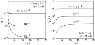
Figure 13: Normalized density of cations $c_{1}(r)=\ell_{B}b^{2}n_{1}(r)$ (left) and anions $c_{2}(r)=\ell_{B}b^{2}n_{2}(r)$ (right) vs $r/b$ with salt at $\ell_{B}\sigma_{0}=1.5$ and $A=0.192$. The salt density is given by $c_{B}=\ell_{B}b^{2}n_{B}=10^{-1},10^{-2}$ and $10^{-3}$ .

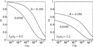
Figure 14: Degree of ionization $\alpha$ as a functions of salt concentration $c_{B}\ell_{B}b^{2}n_{B}$ with salt on a semi-logarithmic scale for $A=0.192$ and $0.0192$. Here $\ell_{B}\sigma_{0}=0.5<1.0$ (left) and $\ell_{B}\sigma_{0}=1.5>1.0$ (right).

We numerically solved the above Poisson-Boltzmann equation and the ionization equation Eq.(2.14) to obtain equilibrium $n_{1}(r)$, $n_{2}(r)$, and $\alpha$. In Fig. 13, we plot the normalized ion densities,

$$c_{1}(r)=\ell_{B}b^{2}n_{1}(r),\quad c_{2}(r)=\ell_{B}b^{2}n_{2}(r),$$ (B3)

which tend to $c_{B}\equiv\ell_{B}b^{2}n_{B}$ for $r\gg k_{D}^{-1}$. We set $\ell_{B}\sigma_{0}=1.5$ and $A=0.192$. Here $c_{1}(r)$ increases and $c_{2}(r)$ decreases near the rod. In Fig. 14, we show $\alpha$ as a function of $c_{B}$ for $\ell_{B}\sigma_{0}=0.5$ and $1.5$. We find that $\alpha$ decreases with increasing the salt concentration $c_{B}$. We also find $\alpha\to 1$ as $c_{B}\to 0$ for $\ell_{B}\sigma_{0}=0.5<1$, while $\alpha$ does not approach unity as $c_{B}\to 0$ for $\ell_{B}\sigma_{0}=1.5>1$. This is consistent with the behavior of $\alpha$ in the limit $M\to\infty$ in the salt-free case discussed in Subsec.IIB. In the limit $c_{B}\to 0$ (with $R=\infty$), $\alpha$ approaches unity for $\ell_{B}\sigma_{0}<1.0$ (though this limiting behavior is not seen for $A=0.0192$ in the left panel), while it tends to a constant in the range $(\ell_{B}\sigma_{0})^{-1}<\alpha<1$ for $\ell_{B}\sigma_{0}>1.0$ as can be seen in the right panel.

Thus, with increasing the salt density, $\alpha$ is reduced and the electrostatic interaction is screened. Experimentally, with addition of salt, highly expanded polyelectrolyte coils have been observed to shrink, eventually resulting in precipitation of the chains (phenomenon known as ”salting out” of polyelectrolytes Volk ).

Appendix C: Water adsorption around hydrophilic ions at small water content

We here present a statistical theory of water adsorption to hydrophilic ionselectro . The system is in the cylindrical cell $b<r<R$ and $0<z<L$. Each solvation shell consists of $\nu$ water molecules, where $\nu=1,\cdots,S$ with $S$ being the maximum number. The binding energy is $Tw_{\nu}$. If $w_{\nu}\gg 1$, the adsorption can be significant even for small bulk water composition $\phi_{B}$ (see Eq.(C8)).

The number of ionized monomers is $N_{I}=L\sigma$. The numbers of $\nu$-clusters composed of $\nu$ water molecules are $\beta_{\nu}N_{I}$. The total number of the hydrated ionized monomers is then $\beta N_{I}$ with

$$\beta=\sum_{\nu}\beta_{\nu}<1.$$ (C1)

The fractions $\beta_{\nu}$ are determined by minimization of the free energy of the form,

$$\frac{F_{s}}{T} = {N_{0}}\phi_{B}(\ln\phi_{B}-1)+N_{I}(1-\beta)\ln(1-\beta)$$ (C2)

$$+N_{I}\sum_{\nu}\beta_{\nu}(\ln\beta_{\nu}-w_{\nu}),$$

where $N_{0}=V/v_{0}$ with $V=\pi(R^{2}-b^{2})L$ being the volume occupied by the solvent. The total number of the water molecules is fixed as

$$N_{0}\phi_{B}+N_{I}\sum_{\nu}\nu\beta_{\nu}=N_{0}\phi_{B}^{0},$$ (C3)

where $\phi_{B}^{0}$ is the volume fraction without adsorption. From $\partial F_{s}/\partial\beta_{\nu}=0$ under Eq.(C3) we obtain

$${\beta_{\nu}} = ({1-\beta})\phi_{B}^{\nu}e^{w_{\nu}},$$ (C4)

$$\beta = 1-1/[1+\sum_{\nu}\phi_{B}^{\nu}e^{w_{\nu}}].$$ (C5)

For $N_{I}\ll N_{0}$ or for $R\gg b$, we may set $\phi^{0}-\phi\ll\phi$ even if $\beta$ approaches unity. We then calculate the excess free energy $\Delta F_{s}=F_{s}-T{N_{0}}\phi_{B}^{0}(\ln\phi_{B}^{0}-1)$ due to the water adsorption. Some calculations give

$$\frac{\Delta F_{s}}{T} = N_{0}\phi_{B}^{0}\ln(\phi_{B}/\phi_{B}^{0})+N_{I}[\phi_{B}^{0}-\phi_{B}+\ln(1-\beta)]$$ (C6)

$$\cong -N_{I}\ln[1+\sum_{\nu}\phi_{B}^{\nu}e^{w_{\nu}}].$$

Here we set $\ln(\phi_{B}/\phi_{B}^{0})\cong\phi_{B}/\phi_{B}^{0}-1$ in the first line to obtain the second line for $N_{I}\ll N_{0}$.

The formation of solvation shells around the counterions may be calculated in the same manner. Let $Tw_{\nu}^{\prime}$ with $\nu=1,\cdots,S^{\prime}$ be the binding energy of $\nu$-clusters of water molecules. For monovalent counterions, we find the free energy decrease in the same form as that in Eq.(C6) with $w_{\nu}$ being replaced by $w_{\nu}^{\prime}$. For a sufficiently small water density outside the solvation shells, we may use the results of one-component solvents in Sec.II if $\Delta_{0}$ is replaced by

$${\tilde{\Delta}}_{0}=\Delta_{0}-\ln\bigg{\{}\bigg{[}1+\sum_{\nu=1}^{S}\phi_{B}^{\nu}e^{w_{\nu}}\bigg{]}\bigg{[}1+\sum_{\nu=1}^{S^{\prime}}\phi_{B}^{\nu}e^{w_{\nu}^{\prime}}\bigg{]}\bigg{\}}.$$ (C7)

The dissociation constant $K_{0}$ in Eq.(2.16) is changed to $\tilde{K}_{0}=n_{01}\exp({-\tilde{\Delta}_{0}})$. and the parameter $A$ in Eq.(2.23) is replaced by $\tilde{A}=2\pi\ell_{B}b^{2}{\tilde{K}}_{0}$.

Let the maximum of $w_{\nu}/\nu$ and $w_{\nu}^{\prime}/\nu$ be $w_{s}$. Significant ionization enhancement occurs for

$$\phi_{B}\gg\exp({-w_{s}}),$$ (C8)

where the right hand side is small for $w_{s}\gg 1$.

References

- (1) G.S. Manning, J. Chem. Phys. 51, 924 (1969); J. Phys. Chem. B 111, 8554 (2007).
- (2) F. Oosawa, Polyelectrolytes (Marcel Dekker, New York, 1971).
- (3) J.L. Barrat and J.F. Joanny, Adv. Chem. Phys. XCIV, I. Prigogine, S.A. Rice Eds., John Wiley Sons, New York 1996.
- (4) Y. Levin, Rep. Prog. Phys. 65, (2002) 1577.
- (5) N. Volk, D. Vollmer, M. Schmidt, W. Oppermann, and K. Huber, Adv. Polym. Sci. 166, 29 (2004).
- (6) C. Holm, J. F. Joanny, K. Kremer, R. R. Netz, P. Reineker, C. Seidel, T. A. Vilgis, and R. G. Winkler, Adv. Polym. Sci. 166, 67 (2004).
- (7) A.V. Dobrynin and M. Rubinstein, Prog. Polym. Sci. 30, 1049 (2005).
- (8) W. Essafi, F. Lafuma, D. Baigl, and C. E. Williams, Europhys. Lett. 71, 938 (2005).
- (9) D. Andelman, Proceeding of the Nato ASI and SUSSP on ”soft condensed matter in molecular and cell biology”, (2005), ed. by W. Poon and D. Andelman, (Taylor & Francis, New York, 2006), pp. 97-122.
- (10) A. Naji and R. R. Netz, Phys. Rev. E 73, 056105 (2006).
- (11) R. Messina, J. Phys.: Condens. Matter 21, 113102 (2009).
- (12) E. Raphael and J. F. Joanny, Europhys. Lett. 13, 623 (1990).
- (13) I. Borukhov, D. Andelman, and H. Orland, Europhys. Lett.32, 499 (1995).
- (14) I. Borukhov, D. Andelman, R. Borrega, M. Cloitre, L. Leibler, and H. Orland, J. Phys. Chem. B 104, 11027 (2000).
- (15) M. Muthukumar, J. Chem. Phys. 120, 9343 (2004).
- (16) Y. Burak and R. R. Netz, J. Phys. Chem. B 108, 4840 (2004). This paper shows that the electrostatic interaction among the charged monomers gives rise to correlated ionization.
- (17) A. Onuki and R. Okamoto, J. Phys. Chem. B, 113, 3988 (2009).
- (18) C. B. Post and B. H. Zimm, Biopolymers 21, 2139 (1982).
- (19) P. G. Arscott, C. Ma, J. R. Wenner and V. A. Bloomfield, Biopolymers, 36, 345 (1995).
- (20) A. Hultgren and D. C. Rau, Biochemistry 43, 8272 (2004).
- (21) C. Stanley and D. C. Rauy, Biophy. J. 91, 912 (2006).
- (22) S. Flock, R. Labarbe, and C. Houssier, Biophysical Journal 70, 1456 (1996).
- (23) D. Baigl and K. Yoshikawa, J. Biophys. 88, 3486 (2005).
- (24) S. M. Mel’nikov, V. G. Sergeyev, and K. Yoshikawa, J. Am. Chem. Soc. 117, 2401 (1995).
- (25) D. Ben-Yaakov, D. Andelman, D. Harries, and R. Podgornik, J. Phys. Chem. B 113 6001 (2009).
- (26) J. N. Israelachvili, Intermolecular and Surface Forces (Academic Press, London, 1991).
- (27) A. Onuki and H. Kitamura, J. Chem. Phys. 121, 3143 (2004).
- (28) A. Onuki, Phys. Rev. E 73, 021506 (2006).
- (29) A. Onuki, J. Chem. Phys. 128, 224704 (2008).
- (30) Y. Tsori and L. Leibler, Proc. Natl. Acad. Sci. U.S.A. 104, 7348 (2007)
- (31) M. Bier, J. Zwanikken, and R. van Roij, Phys. Rev. Lett. 101, 046104 (2008); J. Zwanikken, J. de Graaf, M. Bier, and R. van Roij, J. Phys.: Condens. Matter 20, 494238 (2008).
- (32) A. Onuki, Europhys. Lett. 82, 58002 (2008).
- (33) J. W. Cahn, J. Chem. Phys. 66 3667 (1977).
- (34) C. Ebner and W. F. Saam, Phys. Rev. Lett. 38, 1486 (1977).
- (35) P. Tarazona and R. Evans, Mol. Phys. 48, 799 (1983).
- (36) A. Onuki, Phase Transition Dynamics (Cambridge University Press, Cambridge, 2002)
- (37) R. M. Fuoss, A. Katchalsky, and S. Lifson, Proc. Natl. Acad. Sci. U.S.A., 37, 579 (1951).
- (38) For ideal gases the entropic free energy is of the form with , where is the Planck constant and is the particle mass. This term is larger than that in Eq.(2.7) by , where is a constant shift of the chemcal potential of the th ions.
- (39) T. Osakai and K. Ebina, J. Phys. Chem. B 102, 5691 (1998). In water-nitrobenzene(Nr) in two phase coexistence, they measured the number of hydrating water molecules around ions in a Nr-rich region at room temperatures. The water number per ion in the Nr-rich phase was estimated to be 4 for Na+, 6 for Li+, and 15 for Ca2+, while it was nearly zero for hydrophobic ions. Their experiment demonstrates strong binding of water molecules to hydrophilic ions even at small water contents.
- (40) A. Hamnett, C. H. Hamann, and W. Vielstich, Electrochemistry (Vch Verlagsgesellschaft Mbh, 1998).
- (41) P. Debye and K. Kleboth, J. Chem. Phys. 42, 3155 (1965).
- (42) H. Ohtaki, Bulletin of the Chemical Society of Japan, 42, 1573 (1969).
- (43) D. Bonn, D. Ross, S. Hachem, S. Gridel, and J. Meunier, Europhys. Lett. 58, 74 (2002).
- (44) M. Born, Z. Phys. 1, 45 (1920).
- (45) Le Quoc Hung, J. Electroanal. Chem. 115, 159 (1980).
- (46) G. Marcus, S. Samin, and Y. Tsori, J. Chem. Phys. 129, 061101 (2008). These authors assumed the homogeneity of , where the counerions are absent and the gradient term is neglected. Compare their and our in Eq.(3.11). In their theory, for rods) plays the role of an inhomogeneous ordering field.
- (47) H. Kitamura and A. Onuki, J. Chem. Phys. 123, 124513 (2005).
- (48) P.G. de Gennes, J. Phys. (Paris) 37, 59 (1976). Polymers can interact with two solvent components asymmetrically. There arises a pairwise attractive interaction among the monomers mediated by the critical fluctuations. Similar attractive interactions were derived among ions in mixture solvents by one of the present authorsOnukiPRE .
- (49) A. Dondos and Y. Izumi, Makromol. Chem. 181, 701 (1980); C. A. Grabowski and A. Mukhopadhyay, Phys. Rev. Lett. 98, 207801 (2007).
- (50) T. Sumi, K. Kobayashi, and H. Sekino, J. Chem. Phys. 127, 164904 (2007).
- (51) A. F. Kostko, M. A. Anisimov, and J. V. Sengers, Phys. Rev. E 70, 026118 (2004).
- (52) H. Matsuoka, D. Schwahn, and N. Ise, Macromolecules 24, 4227 (1991).
- (53) J. J. Tanahatoe and M. E. Kuil, J. Phys. Chem. B 101, 5905 (1997).
- (54) B. D. Ermi and E. J. Amis, Macromolecules 31, 7378 (1998).
- (55) K. Sadakane, H. Seto, H. Endo, and M. Shibayama, J. Phys. Soc. Jpn., 76, 113602 (2007); K. Sadakane, A. Onuki, K. Nishida, S. Koizumi, and H. Seto, preprint(arXiv:0903.2303v2).
- (56) K. Shirahama, K. Takashima, and N. Takisawa, Bulletin of the Chemical Society of Japan, 60, 43 (1987).
- (57) K. Tanaka and Y. Okahata, J. Am. Chem. Soc., 118, 10679 (1996).
- (58) P. S. Kuhn, Y. Levin, M. C. Barbosa, Chemical Physics Letters 298, 51 (1998).