Braiding surface links which are coverings over the standard torus

Abstract.

We consider a surface link in the 4-space which can be presented by a simple branched covering over the standard torus, which we call a torus-covering link. Torus-covering links include spun $T^{2}$-knots and turned spun $T^{2}$-knots. In this paper we braid a torus-covering link over the standard 2-sphere. This gives an upper estimate of the braid index of a torus-covering link. In particular we show that the turned spun $T^{2}$-knot of the torus $(2,\,p)$-knot has the braid index four.

1. Introduction

A surface link is the image of a locally flat embedding of a closed surface into the Euclidean 4-space $\mathbb{R}^{4}$. It is known [10, 12] that any oriented surface link can be presented by the closure of a simple surface braid. Here, the closure of a surface braid is a surface link of the following form. Let $S^{2}$ be a standard 2-sphere in $\mathbb{R}^{4}$, i.e. the boundary of a standard 3-ball in $\mathbb{R}^{3}\times\{0\}$. The closure of a surface braid is a surface link embedded in a tubular neighborhood $N(S^{2})$ of $S^{2}$ in such a way that the projection of it to $S^{2}$ is a branched covering over $S^{2}$. We identify $N(S^{2})$ with $I\times I\times S^{2}$, where $I$ is an interval. For a surface link $S$ of such a form, we consider the singular set of the image of $S$ by the projection to $I\times S^{2}$, and the image of this singular set by the projection to $S^{2}$ forms a graph on $S^{2}$. An $m$-chart on $S^{2}$ is such a graph with certain additional data. We can present the original surface link by its $m$-chart on $S^{2}$ ([11, 12]). By removing from $S^{2}$ a 2-disk which is disjoint with the $m$-chart, we obtain an $m$-chart on a 2-disk. The resulting $m$-chart on a 2-disk is called a surface link $m$-chart. As we mentioned, any oriented surface link can be presented by the closure of a simple surface braid. Thus it follows that any oriented surface link is presented by a surface link $m$-chart. In [15], a “torus-covering link” is introduced as a new construction of a surface link, by considering a standard torus instead of a standard 2-sphere. Let $T$ be a standard torus in $\mathbb{R}^{4}$, i.e. the boundary of a standard solid torus in $\mathbb{R}^{3}\times\{0\}$. A torus-covering link is a surface link embedded in a tubular neighborhood $N(T)$ of $T$ in such a way that the projection of it to $T$ is a simple branched covering over $T$. For a surface link of such a form, we can define its $m$-chart on $T$ in the same way as above. By cutting $T$ along a meridian and a longitude, we obtain an $m$-chart on a 2-disk. We will call the resulting $m$-chart on a 2-disk a torus-covering $m$-chart. A torus-covering link is presented by a torus-covering $m$-chart. The aim of this paper is to give a surface link chart description of a torus-covering link $S$, from the torus-covering $m$-chart which presents $S$.

Since a torus-covering link is an oriented surface link, it can be presented by a surface link $m$-chart. We give a surface link chart description of a torus-covering link $S$, from the torus-covering $m$-chart which presents $S$ (Theorem 3.2). In other words, we braid $S$ over a standard 2-sphere. We deform $S$ to the form of the closure of a simple surface braid, using the motion picture method. The braid index of an oriented surface link $F$ is the minimum degree of simple surface braids whose closures in $\mathbb{R}^{4}$ are equivalent to $F$. The resulting surface link chart of Theorem 3.2 is a $2m$-chart; thus we can see that $2m$ is an upper estimate of the braid index of the torus-covering link $S$ (Corollary 4.1). In particular, we show that the turned spun $T^{2}$-knot of the torus $(2,p)$-knot has the braid index four.

The paper is organized as follows. In Section 2, we review the chart description of a simple braided surface, and using these terms we give the definition of a torus-covering link. In Section 3, we give the statement of Theorem 3.2. In Section 4, we prove Theorem 3.2 using the motion picture method. In Section 5, we give an example; we draw the surface link chart presenting the turned spun $T^{2}$-knot of a trefoil.

2. Torus-covering links

In this section we give the definition of a torus-covering link. In Section 2.1 we review a simple braided surface and its chart description, and in Section 2.2 we give the definition of a torus-covering link.

2.1. A braided surface and its chart description

A braided surface was defined in [17, 12]. A surface braid is a braided surface with some boundary condition, and a notion of an $m$-chart was introduced [8, 12] to present a simple surface braid. Equivalent simple surface braids have distinct chart presentations. The notion of C-move equivalence between two $m$-charts was introduced [8, 11, 12] to give the equivalence class of the chart which represents the equivalence class of a simple surface braid. The notion of an $m$-chart can be easily extended to an $m$-chart presenting a simple braided surface. In this subsection we review a braided surface, and extend the notion of a chart description to a simple braided surface.

Definition 2.1.

A compact and oriented 2-manifold $S$ embedded in a bidisk $D_{1}\times D_{2}$ properly and locally flatly is called a braided surface of degree $m$ if $S$ satisfies the following conditions:

1. $p_{2}|_{S}\,:\,S\rightarrow D_{2}$ is a branched covering map of degree $m$,

2. $\partial S$ is a closed $m$-braid in $D_{1}\times\partial D_{2}$, where $D_{1}$, $D_{2}$ are 2-disks, and $p_{2}\,:\,D_{1}\times D_{2}\rightarrow D_{2}$ is the projection to the second factor.

Two braided surfaces are equivalent if there is a fiber-preserving ambient isotopy of $D_{1}\times D_{2}$ rel $D_{1}\times\partial D_{2}$ which carries one to the other. A braided surface $S$ is called simple if $\#(S\cap p_{2}^{-1}(x))=m-1$ or $m$ for each $x\in D_{2}$. A braided surface $S$ is called a surface braid if $\partial S$ is the trivial closed braid. A surface braid $Q_{m}\times D_{2}$ is called trivial, where $Q_{m}$ is a set of $m$ interior points of $D_{1}$.

When a simple braided surface $S$ is given, we obtain a graph on $D_{2}$, as follows. Identify $D_{1}$ with $I\times I$, where $I=[0,1]$. Consider the singular set $\mathrm{Sing}(p_{1}(S))$ of the image of $S$ by the projection $p_{1}$ to $I\times D_{2}$. Perturbing $S$ if necessary, we can assume that $\mathrm{Sing}(p_{1}(S))$ consists of double point curves, triple points, and branch points. Moreover we can assume that the singular set of the image of $\mathrm{Sing}(p_{1}(S))$ by the projection to $D_{2}$ consists of a finite number of double points such that the preimages belong to double point curves of $\mathrm{Sing}(p_{1}(S))$. Thus the image of $\mathrm{Sing}(p_{1}(S))$ by the projection to $D_{2}$ forms a finite graph $\Gamma$ on $D_{2}$ such that the degree of its vertex is either $1$, $4$ or $6$. An edge of $\Gamma$ corresponds to a double point curve, and a vertex of degree $1$ (resp. $6$) corresponds to a branch point (resp. triple point).

For such a graph $\Gamma$ obtained from a simple braided surface $S$, we give orientations and labels to the edges of $\Gamma$, as follows. Let us consider a path $\rho$ in $D_{2}$ such that $\rho\cap\Gamma$ is a point $P$ of an edge $e$ of $\Gamma$. Then $S\cap p_{2}^{-1}(\rho)$ is a classical $m$-braid with one crossing in $p_{2}^{-1}(\rho)$ such that $P$ corresponds to the crossing of the $m$-braid. Let $\sigma_{1},\sigma_{2},\ldots,\sigma_{m-1}$ be the standard generators of the $m$-braid group $B_{m}$. Let $\sigma_{i}^{\epsilon}$ ($i\in\{1,2,\ldots,m-1\}$, $\epsilon\in\{+1,-1\}$) be the presentation of $S\cap p_{2}^{-1}(\rho)$. Then label the edge $e$ by $i$, and moreover give $e$ an orientation such that the normal vector of $\rho$ corresponds (resp. does not correspond) to the orientation of $e$ if $\epsilon=+1$ (resp. $-1$). We call such an oriented and labeled graph an $m$-chart of $S$.

In general, we define an $m$-chart on $D_{2}$ as follows.

Definition 2.2.

Let $m$ be a positive integer. A finite graph $\Gamma$ on a 2-disk $D_{2}$ is called an $m$-chart if it satisfies the following conditions:

1. $\Gamma\cap\partial D_{2}$ consists of a finite number of vertices of degree $1$.

2. Every edge is oriented and labeled by an element of $\{1,2,\ldots,m-1\}$.

3. Every vertex has degree $1$, $4$, or $6$.

4. The adjacent edges around each vertex in $\mathrm{Int}(D_{2})$ are oriented and labeled as shown in Figure 1, where we depict a vertex of degree 1 by a black vertex, and a vertex of degree 6 by a white vertex.

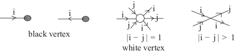
Figure 1. Vertices in a chart.

A black vertex (resp. white vertex) of an $m$-chart corresponds to a branch point (resp. triple point) of the simple braided surface presented by the $m$-chart. An $m$-chart presents a simple braided surface. In particular, an $m$-chart $\Gamma$ such that $\Gamma\cap\partial D_{2}=\emptyset$ presents a simple surface braid.

When an $m$-chart $\Gamma$ on $D_{2}$ is given, we can reconstruct a simple braided surface $S$ over $D_{2}$ as follows. Let $N(\Gamma)$ be a neighborhood of $\Gamma$ in $D_{2}$. Let us consider a trivial braided surface $S=Q_{m}\times(D_{2}-N(\Gamma))$ over $D_{2}-N(\Gamma)$, where $Q_{m}$ is a set of $m$ interior points of $D_{1}$. We extend $S$ over a neighborhood of each edge as follows. Identify a neighborhood of an edge $e$ with $I\times I$ such that $e$ is identified with $\{1/2\}\times I$. Let $i$ be the label attached to $e$, and let $\epsilon=+1$ (resp. $-1$) if the orientation of $e$ corresponds (resp. does not correspond) to the orientation of $\{0\}\times I$. Then let the braided surface $S$ over the neighborhood of $e$ be the braided surface which has a presentation $\sigma_{i}^{\epsilon}\times I$ and the image of the double point curve of $p_{1}(S)$ by the projection to $D_{2}$ is $e$. Since $\Gamma$ is as in Figure 1 around each vertex, $S$ can be extended naturally over a neighborhood of each vertex. See [4, 9, 12] for more details. Thus we can construct a simple braided surface $S$ over $D_{2}$ such that the original $m$-chart is an $m$-chart of $S$.

Two $m$-charts on $D_{2}$ are C-move equivalent if they are related by a finite sequence of ambient isotopies of $D_{2}$ and CI, CII, CIII-moves shown in Figure 2; see [12] for the complete set of CI-moves. It is shown as a minor modification of [8, 11, 12] that two simple braided surfaces of degree $m$ are equivalent if and only if $m$-charts of them are C-move equivalent.

The boundary of a surface braid $S$ consists of trivial closed $m$-braid. Consider a natural embedding of $D_{1}\times D_{2}$ in $\mathbb{R}^{4}$, and paste $m$ disks to $S$ to obtain an embedding of a closed surface in $\mathbb{R}^{4}$. The resulting surface is called the closure of $S$ (see Section 4). It is known [10, 12] that any oriented surface link is presented by the closure of a simple surface braid; thus it is presented by an $m$-chart $\Gamma$ on a 2-disk $D_{2}$ such that $\Gamma\cap D_{2}=\emptyset$. We call such an $m$-chart which presents a surface link a surface link $m$-chart.

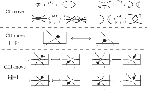
Figure 2. CI, CII, CIII-moves. For CI-moves, we give only several examples.

2.2. Torus-covering links

Now we give the definition of a torus-covering link in $\mathbb{R}^{4}$ (see [15, Definition 2.1]). Let $T$ be a standard torus in $\mathbb{R}^{4}$, that is, the boundary of an unknotted solid torus in a 3-space in $\mathbb{R}^{4}$. Let us consider a tubular neighborhood $N(T)$ of $T$, and identify $N(T)$ with $D^{2}\times S^{1}\times S^{1}$, where $D^{2}$ is a 2-disk, and $S^{1}$ is a circle. The first $S^{1}$ corresponds to the meridian, and the second $S^{1}$ corresponds to the longitude of $T$. Let us identify $S^{1}$ with $I/\sim$, where $I=[0,\,1]$ and $0\sim 1$. For a manifold $S$ in $N(T)$, let us denote by $S\cap(D^{2}\times I\times I)$ the manifold in $D^{2}\times I\times I$ obtained from $S$ by cutting it at $D^{2}\times S^{1}\times\{0\}$ and $D^{2}\times\{0\}\times S^{1}$.

Definition 2.3.

A torus-covering link is a surface link $S$ in $\mathbb{R}^{4}$ such that $S\subset N(T)$ and moreover $S\cap(D^{2}\times I\times I)$ is a simple braided surface.

By definition, a torus-covering link $S$ is presented by an $m$-chart $\Gamma$ on $I\times I$ with $\Gamma\cap(I\times\{0\})=\Gamma\cap(I\times\{1\})$ and $\Gamma\cap(\{0\}\times I)=\Gamma\cap(\{1\}\times I)$. Let us call $\Gamma$ on $I\times I$ a torus-covering $m$-chart.

As we mentioned, for two $m$-charts, their presenting braided surfaces are equivalent if the $m$-charts are C-move equivalent. Hence it follows that for two torus-covering $m$-charts, their presenting torus-covering links are equivalent if the torus-covering $m$-charts are C-move equivalent. Since each component of a torus-covering link is a branched cover over a torus $T$, each component of a torus-covering link is of genus at least one.

A $T^{2}$-link is a surface link whose each component is of genus one. As known $T^{2}$-links constructed from classical links, there are spun $T^{2}$-links and turned spun $T^{2}$-links, which are constructed as follows. Consider a 3-ball $B^{3}$ and a natural embedding of $B^{3}\times S^{1}$ in $\mathbb{R}^{4}$. The space $B^{3}\times S^{1}$ can be regarded as constructed by spinning $B^{3}$ along the circle $S^{1}$. A spun $T^{2}$-link of a classical link $L$ is constructed by spinning $L\subset B^{3}$ ([14, 2, 3]). A turned spun $T^{2}$-link of $L$ is constructed by turning $L\subset B^{3}$ once while spinning ([3]). A spun $T^{2}$-link or a turned spun $T^{2}$-link of any classical closed braid is presented by a torus-covering link (see [15, Propositions 2.10 and 2.11]).

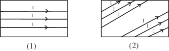
Figure 3. Examples of $2$-charts on $T$, or torus-covering $2$-charts on a 2-disk.

Example 2.4.

1. Let $\Gamma$ be a torus-covering 2-chart as in Figure 3 (1). Then the torus-covering knot presented by $\Gamma$ is the spun $T^{2}$-knot of a right-handed trefoil.

2. Let $\Gamma$ be a torus-covering 2-chart as in Figure 3 (2). Then the torus-covering knot presented by $\Gamma$ is the turned spun $T^{2}$-knot of a right-handed trefoil.

3. Braiding a torus-covering link over the 2-sphere

In this section we give the statement of Theorem 3.2, using the terms of $m$-charts. An $m$-chart is presented by a simple braided surface. A simple braided surface is presented by a motion picture consisting of isotopic transformations and hyperbolic transformations (see [12, Section 9.1]).

For a subset $A_{1}$ of $\mathbb{R}^{3}$ and a subset $A_{2}$ of $\mathbb{R}$, we denote by $A_{1}A_{2}$ (or by $A_{1}\times A_{2})$ the subset $\{(x,t)\in\mathbb{R}^{3}\times\mathbb{R}\,|\,x\in A_{1},\,t\in A_{2}\}$ of $\mathbb{R}^{3}\times\mathbb{R}=\mathbb{R}^{4}$. In particular, when $A_{2}=\{t\}$, we denote $A_{1}\{t\}$ by $A_{1}[t]$. For a subset $X$ of $\mathbb{R}^{4}=\mathbb{R}^{3}\times\mathbb{R}$, a motion picture of $X$ is a one-parameter family $\{\pi(X\cap\mathbb{R}^{3}[t])\}_{t\in\mathbb{R}}$, where $\pi\,:\,\mathbb{R}^{4}\rightarrow\mathbb{R}^{3}$, $\pi(x,y,z,t)=(x,y,z)$ is the projection.

Let $\{h_{t}\}_{t\in[0,1]}$ be an ambient isotopy of $\mathbb{R}^{3}$. For a classical link $L$, we have an isotopy (a one-parameter family) $\{h_{t}(L)\}$ of classical links. We say that $h_{1}(L)$ is obtained from $L$ by an isotopic transformation, and use the notation that $L\rightarrow h_{1}(L)$ is an isotopic transformation.

Let $L$ be a classical link in $\mathbb{R}^{3}$. A 2-disk $B$ in $\mathbb{R}^{3}$ is called a band attaching to $L$ if $L\cap B$ is a pair of disjoint arcs in $\partial B$. A band set attaching to $L$ is a union $\mathcal{B}=B_{1}\cup B_{2}\cup\cdots\cup B_{m}$ of mutually disjoint bands $B_{1},B_{2},\cdots,B_{m}$ attaching to $L$. For a subset $X$ of a space, let us denote by $\mathrm{Cl}(X)$ the closure of $X$. Define a link $h(L;\mathcal{B})$ by

$$h(L;\mathcal{B})=\mathrm{Cl}\big{(}(L\cup\partial\mathcal{B})-(L\cap\mathcal{B})\big{)}.$$

We say that the link $h(L;\mathcal{B})$ is obtained from $L$ by a hyperbolic transformation along $\mathcal{B}$, and use the notation that $L\rightarrow h(L;\mathcal{B})$ is a hyperbolic transformation (see [12, Section 9.1]).

For a classical $m$-braid $c$, let $\iota^{l}_{k}(c)$ be the $(m+k+l)$-braid obtained from $c$ by adding $k$ (resp. $l$) trivial strings before (resp. after) $c$, and put

$$\Pi^{m}_{i}=\sigma_{m+1}\sigma_{m+2}\cdots\sigma_{m+i},\ \Pi^{\prime\,m}_{i}=\sigma_{m-1}\sigma_{m-2}\cdots\sigma_{m-i},$$

$$\Delta_{m}=\Pi^{m}_{m-1}\Pi^{m}_{m-2}\cdots\Pi^{m}_{1},\ \Delta_{m}^{\prime}=\Pi^{\prime\,m}_{m-1}\Pi^{\prime\,m}_{m-2}\cdots\Pi^{\prime\,m}_{1},$$

$$\Theta_{m}=\sigma_{m}\cdot\Pi^{\prime\,m}_{m-1}\cdot\Pi^{m}_{m-1}\cdot\sigma_{m}\cdot\Pi^{\prime\,m}_{m-2}\cdot\Pi^{m}_{m-2}\cdots\sigma_{m}\cdot\Pi^{\prime\,m}_{1}\cdot\Pi^{m}_{1}\cdot\sigma_{m}.$$

Remark 3.1.

Let $\Delta$ be Garside’s $\Delta$ (a half twist, see [5]) for the $m$-braid group $B_{m}$. Then $\iota^{0}_{m}(\Delta)=\Delta_{m}$.

Theorem 3.2.

Let $\Gamma_{T}$ be a torus-covering $m$-chart. Let $a$ (resp. $b$) be a classical $m$-braid presented by $\Gamma_{T}\cap(I\times\{0\})$ (resp. $\Gamma_{T}\cap(\{0\}\times I)$). Then the torus-covering link presented by $\Gamma_{T}$ is presented by a surface link $2m$-chart $\Gamma_{S}$ as in Figure 4. Here $H_{b}$ is a $2m$-chart presenting the simple braided surface whose motion picture is as follows:

$$\iota^{m}_{0}(b) \longrightarrow \iota^{m}_{0}(b)\cdot(\Delta^{\prime}_{m})^{-1}\cdot\Delta_{m}^{-1}\cdot\Delta^{\prime}_{m}\cdot\Delta_{m}\dot{\longrightarrow}\iota^{m}_{0}(b)\cdot(\Delta^{\prime}_{m})^{-1}\cdot\Delta^{-1}_{m}\cdot\Theta_{m}$$

$$\longrightarrow (\Delta^{\prime}_{m})^{-1}\cdot\Delta^{-1}_{m}\cdot\iota^{m}_{0}(\bar{b}^{*})\cdot\Theta_{m}\longrightarrow(\Delta^{\prime}_{m})^{-1}\cdot\Delta^{-1}_{m}\cdot\Theta_{m}\cdot\iota^{0}_{m}(\bar{b}^{*})$$

$$\dot{\longrightarrow} (\Delta^{\prime}_{m})^{-1}\cdot\Delta^{-1}_{m}\cdot\Delta^{\prime}_{m}\cdot\Delta_{m}\cdot\iota^{0}_{m}(\bar{b}^{*})\longrightarrow\iota^{0}_{m}(\bar{b}^{*}),$$

where $\longrightarrow$ is an isotopic transformation and $\dot{\longrightarrow}$ is a hyperbolic transformation along bands corresponding to the $m\ \sigma_{m}$’s (see Figure 5), and $-(H_{b})^{*}$ is the orientation-reversed mirror image of $H_{b}$, and $\bar{b}^{*}$ is the $m$-braid obtained from the classical $m$-braid $b$ by taking its mirror image and reversing all the crossings (see Figure 6).

Definition 3.3.

Let us call $H_{b}$ the 1-handle $2m$-chart associated with an $m$-braid $b$, and its presenting braided surface the 1-handle braided surface.

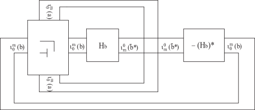
Figure 4. The surface link $2m$-chart $\Gamma_{S}$.

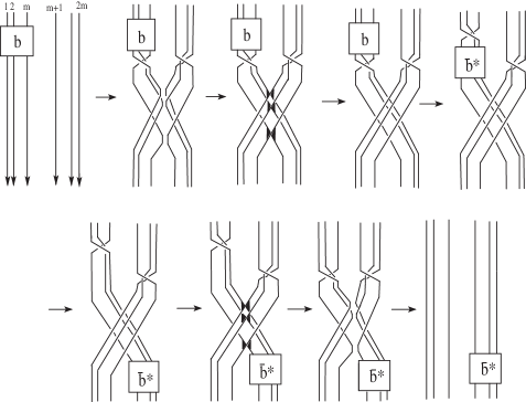
Figure 5. The motion picture of the 1-handle braided surface (of degree $2m$) associated with an $m$-braid $b$.

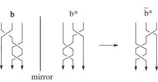
Figure 6. The $m$-braid $\bar{b}^{*}$.

The surface link $2m$-chart $\Gamma_{S}$ is well-defined, for the edges presenting $\iota^{m}_{0}(a)$ have labels at most $m-1$ and the edges presenting $\iota^{0}_{m}(\bar{b}^{*})$ have labels at least $m+1$. Note that the 1-handle $2m$-chart $H_{b}$ has $2m$ black vertices.

4. Proof of Theorem 3.2

Before proving Theorem 3.2, we review the Cellular Move Lemma and the definition of the closure of a surface braid.

Let $F$ be a surface link and let $E^{3}$ be a 3-ball in $\mathbb{R}^{4}$. Suppose that $E^{3}\cap F$ is a 2-disk in $\partial E^{3}$. Replacing $E^{3}\cap F$ by the 2-disk $\mathrm{Cl}\big{(}\partial E^{3}-(E^{3}\cap F)\big{)}$, we obtain a new surface link $F^{\prime}$ from $F$. Such a replacement is called a cellular move along $E^{3}$. If $F$ is oriented, then we assume that $F^{\prime}$ is oriented by an orientation induced from $\mathrm{Cl}\big{(}F-(E^{3}\cap F)\big{)}$. It is known that $F$ and $F^{\prime}$ are equivalent (Cellular Move Lemma, see [12, Lemma 6.6] or [16]).

Assume that $L$ is a trivial classical link, and take $t\in\mathbb{R}$. A disk system in $\mathbb{R}^{3}(-\infty,t]$ (resp. $\mathbb{R}^{3}[t,+\infty)$) with boundary $L[t]$ is a union of mutually disjoint 2-disks embedded in $\mathbb{R}^{3}(-\infty,t]$ (resp. $\mathbb{R}^{3}[t,+\infty)$) properly and locally flatly such that the boundary is $L[t]$. A disk system $\tilde{\mathcal{D}}$ in $\mathbb{R}^{3}(-\infty,t]$ (resp. $\mathbb{R}^{3}[t,+\infty)$) is trivial if there is no critical point except a single minimal point or minimal disk (resp. a maximal point or maximal disk) on each disk component of $\tilde{\mathcal{D}}$ (see [12, Section 8.5]).

Let $t_{1},t_{2}\in\mathbb{R}$ such that $t_{1}<t_{2}$. Let $F$ be a properly embedded surface in $\mathbb{R}^{3}[t_{1},t_{2}]$ and let $L_{-}$ and $L_{+}$ be links in $\mathbb{R}^{3}$ such that $L_{-}$ (resp. $L_{+}$) appears as the boundary of $F$ in $\mathbb{R}^{3}[t_{1}]$ (resp. $\mathbb{R}^{3}[t_{2}]$). When $L_{-}$ and $L_{+}$ are trivial links, we can consider a closed surface $\hat{F}$ such that

$$\hat{F}=\tilde{\mathcal{D}}_{-}\cup F\cup\tilde{\mathcal{D}}_{+},$$

where $\tilde{\mathcal{D}}_{-}$ (resp. $\tilde{\mathcal{D}}_{+}$) is a trivial disk system in $\mathbb{R}^{3}(-\infty,t_{1}]$ (resp. $\mathbb{R}^{3}[t_{2},+\infty)$) with boundary $L_{-}[t_{1}]$ (resp. $L_{+}[t_{2}]$). We call $\hat{F}$ the closure of $F$. It is known [12, Proposition 9.11] that for two closures of $F$, they are ambient isotopic in $\mathbb{R}^{4}$ rel $\mathbb{R}^{3}[t_{1},t_{2}]$. Let $S$ be a surface braid in $D^{2}\times I\times I^{\prime}$, where $D^{2}$ is a 2-disk, $I=[0,1]$ and $I^{\prime}$ is an arbitrary interval. Let us consider a map

(4.1) $$A\,:\,D^{2}\times I\times I^{\prime}\rightarrow D^{2}\times I\times I^{\prime}/(x,0,u)\sim(x,1,u)\subset\mathbb{R}^{3}\times I^{\prime}$$

($x\in D^{2}$ and $u\in I^{\prime}$), where $A(D^{2}\times I\times I^{\prime})=D^{2}\times S^{1}\times I^{\prime}\subset\mathbb{R}^{3}\times I^{\prime}$ is a natural embedding, i.e. $D^{2}\times S^{1}$ is naturally embedded in $\mathbb{R}^{3}$. The image $A(S)$ is embedded in $\mathbb{R}^{3}\times I^{\prime}$ properly and locally flatly. The closure of the surface braid $S$ is the closure of $A(S)$.

Proof of Theorem 3.2. Let $S$ be the torus-covering link presented by a torus-covering $m$-chart $\Gamma_{T}$, and let $\pi\,:\,\mathbb{R}^{4}\rightarrow\mathbb{R}^{3}$, $\pi(x,y,z,t)=(x,y,z)$ be the projection. Let us consider the motion picture $\{S_{t}\}_{t\in\mathbb{R}}$ of $S$, where $S_{t}=\pi(S\cap\mathbb{R}^{3}[t])$. We will draw the figures of $S_{t}$ as the diagrams projected on the xy-plane. We will use the same notation $S$ after each equivalent deformation. For a braid $c$, let us denote by $\mathrm{cl}(c)$ the closed braid associated with $c$.

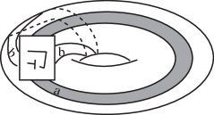
Figure 7. The torus-covering link $S$.

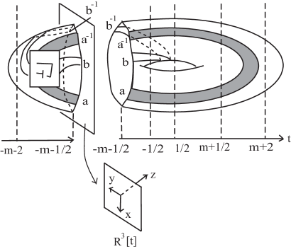
Figure 8. The torus-covering link $S$.

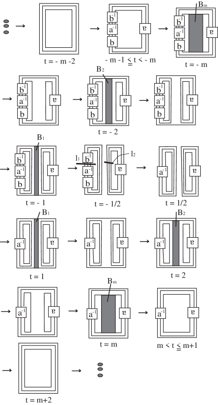
Figure 9. Motion picture of $S$ (1).

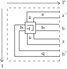
Figure 10. The $m$-chart $\Gamma_{T}^{\prime}$.

Step 1.  Let us consider the standard torus $T$ in the $xyt$-space with $\Gamma_{T}$ on it (see Figure 7). We can assume that $T$ with $\Gamma_{T}$ is as in Figure 8. Then the motion picture of $S$ is as in Figure 9, as follows.

Let $B_{1},B_{2},\ldots,B_{m}$ be $m$ bands in $\mathbb{R}^{3}$ such that $B_{j}[-j]$ (resp. $B_{j}[j]$) is an untwisted band attaching to $S_{-j-1/2}[-j]\subset\mathbb{R}^{3}[-j]$ (resp. $S_{j-1/2}[j]\subset\mathbb{R}^{3}[j]$) as in Figure 9 ($j=1,2,\ldots,m$). Let us denote by $e_{m}$ the trivial $m$-braid. Let $\tilde{\mathcal{D}}_{-,m}$ (resp. $\tilde{\mathcal{D}}_{+,m}$) be a trivial disk system of $m$ components in $\mathbb{R}^{3}(-\infty,t]$ (resp. $\mathbb{R}^{3}[t,+\infty)$) with boundary $\mathrm{cl}(e_{m})[t]$, where $t\in\mathbb{R}$. Let $\Gamma_{T}^{\prime}$ be an $m$-chart on $I\times I^{\prime}$ as in Figure 10, and let $S(\Gamma_{T}^{\prime})$ be the simple braided surface of degree $m$ in $D^{2}\times I\times I^{\prime}$ presented by $\Gamma_{T}^{\prime}$. Then let us consider $A(S(\Gamma_{T}^{\prime}))$, where $A\,:\,D^{2}\times I\times I^{\prime}\rightarrow\mathbb{R}^{3}\times I^{\prime}$ is the map (4.1), and denote this by $A(\Gamma_{T})$. Note that $A(\Gamma_{T})$ is embedded in $\mathbb{R}^{3}\times I^{\prime}$ properly and locally flatly. Let us call $A(\Gamma_{T})$ the braided surface over an annulus associated with $\Gamma_{T}$. Let us consider an $m$-chart $\Gamma$. Let $\rho$ be a path which intersects with the edges of $\Gamma$ transversely. Let $c=\sigma_{i_{1}}^{\epsilon_{i_{1}}}\sigma_{i_{2}}^{\epsilon_{i_{2}}}\cdots\sigma_{i_{\nu}}^{\epsilon_{i_{\nu}}}$ be the $m$-braid presented by $\rho\cap\Gamma$. Let us consider the orientation-reversed path of $\rho$, and denote it by $-\rho$. Then $-\rho\cap\Gamma$ presents $\sigma_{i_{\nu}}^{-\epsilon_{i_{\nu}}}\sigma_{i_{\nu-1}}^{-\epsilon_{i_{\nu-1}}}\cdots\sigma_{i_{1}}^{-\epsilon_{i_{1}}}$, which is $c^{-1}$. Hence the classical $m$-braid $S(\Gamma_{T}^{\prime})\cap(D^{2}\times I\times\{t\})$ is $a^{-1}bab^{-1}$, where $\{t\}$ is the point of $\partial I^{\prime}$ with the greater coordinate.

Let $l_{1}$ (resp. $l_{2}$) $\subset\mathbb{R}^{3}$ be a half plane indicated at $t=-1/2$ in Figure 9. Let us take the identified corresponding ends of a closed braid in $l_{1}$ (resp. $l_{1}\cup l_{2}$) for $t\in[-m-2,\,-m)\cup(m,\,m+2]$ (resp. $t\in(-1,1)$). Then the motion picture depicted in Figure 9, which describes $S$ presented by $\Gamma_{T}$, is as follows. A split union of two classical links $L_{1}$ and $L_{2}$ in $\mathbb{R}^{3}$ is a classical link presented by the union of the copies of $L_{1}$ and $L_{2}$ such that for a 2-sphere $S^{2}$ embedded in $\mathbb{R}^{3}$, $L_{1}$ is inside of $S^{2}$ and $L_{2}$ is outside. We use $\cup$ for a split union of classical links.

1. $S\cap\mathbb{R}^{3}(-\infty,-m-2]=\tilde{\mathcal{D}}_{-,m}$. We have $S_{-m-2}=\mathrm{cl}(e_{m})$.

2. $S\cap\mathbb{R}^{3}[-m-2,-m-1]=A(\Gamma_{T})$ such that $S_{-m-1}=\mathrm{cl}(a^{-1}bab^{-1})$.

3. $S_{t}=S_{-m-1}$, for $t\in[-m-1,\,-m-1/2]$.

4. $S_{-j-1/2}\rightarrow S_{-j+1/2}$ is a hyperbolic transformation along the band $B_{j}\subset S_{-j}$, where $j=1,2,\ldots,m$. We have $S_{-1/2}=\mathrm{cl}(a^{-1}bb^{-1})\cup\mathrm{cl}(a)$.

5. $S_{-1/2}\rightarrow S_{1/2}$ is an isotopic transformation such that $S_{1/2}=\mathrm{cl}(a^{-1})\cup\mathrm{cl}(a)$.

6. $S_{j-1/2}\rightarrow S_{j+1/2}$ is a hyperbolic transformation along the band $B_{j}\subset S_{j}$, where $j=1,2,\ldots,m$. We have $S_{m+1/2}=\mathrm{cl}(a^{-1}a)$.

7. $S_{t}=S_{m+1/2}$ for $t\in[m+1/2,m+1]$.

8. $S_{m+1}\rightarrow S_{m+2}$ is an isotopic transformation such that $S_{m+2}=\mathrm{cl}(e_{m})$.

9. $S\cap\mathbb{R}^{3}[m+2,+\infty)=\tilde{\mathcal{D}}_{+,m}$.

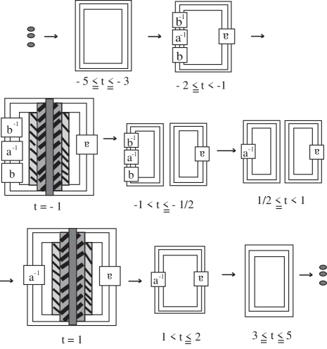
Figure 11. Motion picture of $S$ (2).

Step 2.  Now, let us move bands $B_{2}[-2],B_{3}[-3],\ldots,B_{m}[-m]$ (resp. $B_{2}[2],B_{3}[3],\ldots,B_{m}[m]$) into $\mathbb{R}^{3}[-1]$ (resp. $\mathbb{R}^{3}[1]$) as follows. For subsets $X$ and $Y$ of the $xyz$-space $\mathbb{R}^{3}$, we will say $X$ is over $Y$ with respect to the $z$-axis if for any pair $((x,y,z_{1}),(x,y,z_{2}))\in X\times Y$, $z_{1}>z_{2}$ holds.

Now we can assume that $B_{j-1}$ is over $B_{j}$ with respect to the $z$-axis, where $j=2,3,\ldots,m$. Let us consider 3-balls $V_{2}^{\epsilon},V_{3}^{\epsilon},\ldots,V_{m}^{\epsilon}$ ($\epsilon=-1,+1$) in $\mathbb{R}^{4}$ such that

$$\pi(V_{j}^{\epsilon}\cap\mathbb{R}^{3}[t])=\begin{cases}B_{j}&\mathrm{for}\ t\in[-j,-1]\ \mathrm{if}\ \epsilon=-1,\ \mathrm{or}\\ &\mathrm{for}\ t\in[1,j]\ \mathrm{if}\ \epsilon=+1,\\ \emptyset&\mathrm{otherwise},\end{cases}$$

where $j=2,3,\ldots,m$. Since $B_{j-1}$ is over $B_{j}$ with respect to the $z$-axis, we can see that $V_{2}^{\epsilon},V_{3}^{\epsilon},\ldots,V_{m}^{\epsilon}$ are mutually disjoint and $V_{j}^{\epsilon}\cap S$ is the 2-disk $B_{j}[\epsilon j]\subset\mathbb{R}^{3}[\epsilon j]$, which is in $\partial V_{j}^{\epsilon}$, where $\epsilon=-1,+1$, $j=2,3,\ldots,m$. Hence, by cellular moves along the 3-balls $V_{2}^{\epsilon},V_{3}^{\epsilon},\ldots,V_{m}^{\epsilon}$, we have a band set $\mathcal{B}_{1}[\epsilon]$ in $\mathbb{R}^{3}[\epsilon]$ ($\epsilon=-1,+1$), where $\mathcal{B}_{1}=B_{1}\cup B_{2}\cup\cdots\cup B_{m}$. Let us use the same notation $S$ for the new surface link obtained from $S$ by the cellular moves. By the Cellular Move Lemma, they are equivalent. Then we have the motion picture of $S$ as follows:

1. $S\cap\mathbb{R}^{3}(-\infty,-m-2]=\tilde{\mathcal{D}}_{-,m}$. We have $S_{-m-2}=\mathrm{cl}(e_{m})$.

2. $S\cap\mathbb{R}^{3}[-m-2,-m-1]=A(\Gamma_{T})$. We have $S_{-m-1}=\mathrm{cl}(a^{-1}bab^{-1})$.

3. $S_{-m-1}\rightarrow S_{-1/2}$ is a hyperbolic transformation along the band set $\mathcal{B}_{1}\subset S_{-1}$. We have $S_{-1/2}=\mathrm{cl}(a^{-1}bb^{-1})\cup\mathrm{cl}(a)$.

4. $S_{-1/2}\rightarrow S_{1/2}$ is an isotopic transformation such that $S_{1/2}=\mathrm{cl}(a^{-1})\cup\mathrm{cl}(a)$.

5. $S_{1/2}\rightarrow S_{m+1}$ is a hyperbolic transformation along the band set $\mathcal{B}_{1}\subset S_{1}$. We have $S_{m+1}=\mathrm{cl}(a^{-1}a)$.

6. $S_{m+1}\rightarrow S_{m+2}$ is an isotopic transformation such that $S_{m+2}=\mathrm{cl}(e_{m})$.

7. $S\cap\mathbb{R}^{3}[m+2,+\infty)=\tilde{\mathcal{D}}_{+,m}$.

Then, by an ambient isotopy of $\mathbb{R}^{4}$ rel $\mathbb{R}^{3}[-2,2]$, we can deform $S$ to have the motion picture as in Figure 11, which is as follows:

1. $S\cap\mathbb{R}^{3}(-\infty,-5]=\tilde{\mathcal{D}}_{-,m}$. We have $S_{-5}=\mathrm{cl}(e_{m})$.

2. $S_{t}=S_{-5}$ for $t\in[-5,-3]$.

3. $S\cap\mathbb{R}^{3}[-3,-2]=A(\Gamma_{T})$. We have $S_{-2}=\mathrm{cl}(a^{-1}bab^{-1})$.

4. $S_{-2}\rightarrow S_{-1/2}$ is a hyperbolic transformation along the band set $\mathcal{B}_{1}\subset S_{-1}$. We have $S_{-1/2}=\mathrm{cl}(a^{-1}bb^{-1})\cup\mathrm{cl}(a)$.

5. $S_{-1/2}\rightarrow S_{1/2}$ is an isotopic transformation such that $S_{1/2}=\mathrm{cl}(a^{-1})\cup\mathrm{cl}(a)$.

6. $S_{1/2}\rightarrow S_{2}$ is a hyperbolic transformation along the band set $\mathcal{B}_{1}\subset S_{1}$. We have $S_{2}=\mathrm{cl}(a^{-1}a)$.

7. $S_{2}\rightarrow S_{3}$ is an isotopic transformation such that $S_{3}=\mathrm{cl}(e_{m})$.

8. $S_{t}=S_{3}$ for $t\in[3,5]$.

9. $S\cap\mathbb{R}^{3}[5,+\infty)=\tilde{\mathcal{D}}_{+,m}$.

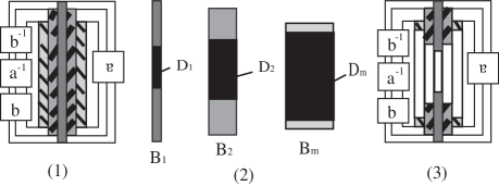
Figure 12. (1) $S_{-1}$ before the cellular moves; (2) 2-disks $D_{i}$ in $B_{i}$; (3) $S_{-1}$ after the cellular moves.

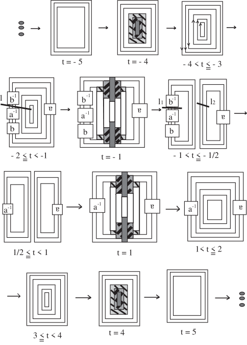
Figure 13. Motion picture of $S$ (3).

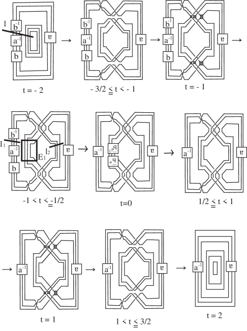
Figure 14. Motion picture of $S\cap\mathbb{R}^{3}[-2,2]$ (4).

Step 3.  We will show that $S$ is equivalent to the surface link whose motion picture $\{S_{t}\}$ is as in Figure 13 for $t\in(-\infty,-2)\cup(2,+\infty)$, and otherwise as in Figure 14.

Let us take 2-disks $D_{1},D_{2},\ldots,D_{m}$ in $\mathbb{R}^{3}$ such that $D_{j}\subset B_{j}$ and $\mathrm{Cl}(B_{j}-D_{j})$ consists of two 2-disks such that each contains one of the two disjoint arcs of $S_{-3/2}\cap B_{j}$; see (2) of Figure 12. Let $W_{j}^{\epsilon}$ ($\epsilon=-1,+1$) be a 3-ball in $\mathbb{R}^{4}$ such that

$$\pi(W_{j}^{\epsilon}\cap\mathbb{R}^{3}[t])=\begin{cases}D_{j}&\mathrm{for}\ t\in[-4,-1]\ \mathrm{if}\ \epsilon=-1,\ \mathrm{or}\\ &\mathrm{for}\ t\in[1,4]\ \mathrm{if}\ \epsilon=+1,\\ \emptyset&\mathrm{otherwise},\end{cases}$$

where $j=1,2,\ldots,m$. Since $B_{1},B_{2},\ldots,B_{m}$ are mutually disjoint, so are $D_{1},D_{2},\ldots,D_{m}$; thus $W_{1}^{\epsilon},W_{2}^{\epsilon},\ldots,W_{m}^{\epsilon}$ are mutually disjoint. Moreover we can see that $W_{j}^{\epsilon}\cap S$ is the 2-disk $D_{j}[\epsilon]\subset\mathbb{R}^{3}[\epsilon]$, which is in $\partial W_{j}^{\epsilon}$, where $\epsilon=-1,+1$, $j=1,2,\ldots,m$. By cellular moves along the 3-balls $W_{1}^{\epsilon},W_{2}^{\epsilon},\ldots,W_{m}^{\epsilon}$ ($\epsilon=-1,+1$), we have $S$ whose motion picture is as in Figure 13. Figure 12 shows (1) $S_{-1}$ before the cellular moves, (2) 2-disks $D_{1},D_{2},\ldots,D_{m}$ in $B_{1},B_{2},\ldots,B_{m}$, and (3) $S_{-1}$ after the cellular moves. Put $\mathcal{B}_{2}=\mathrm{Cl}(B_{1}-D_{1})\cup\mathrm{Cl}(B_{2}-D_{2})\cup\cdots\cup\mathrm{Cl}(B_{m}-D_{m})$, which is a band set in $\mathbb{R}^{3}$ consisting of $2m$ bands. Then the motion picture of $S$ as in Figure 13 is as follows. Let $-\tilde{\mathcal{D}}_{-,m}$, $-\tilde{\mathcal{D}}_{+,m}$, or $-\mathrm{cl}(e_{m})$ be the orientation-reversed image of $\tilde{\mathcal{D}}_{-,m}$, $\tilde{\mathcal{D}}_{+,m}$ or $\mathrm{cl}(e_{m})$ respectively. For an $m$-braid $c$, let us denote by $\iota c$ the braid $\iota_{m}^{0}(c)-e_{m}$, and by $-\iota\tilde{\mathcal{D}}_{-,m}$ (resp. $-\iota\tilde{\mathcal{D}}_{+,m}$) the trivial disk system of $m$ components in $\mathbb{R}^{3}(-\infty,t]$ (resp. $\mathbb{R}^{3}[t,+\infty)$) with boundary $-\iota e_{m}[t]$, where $t\in\mathbb{R}$. Let $l$ (resp. $l_{1}$, $l_{2}$) $\subset\mathbb{R}^{3}$ be a half plane indicated at $t=-2$ (resp. $-1/2$) in Figure 13. Let us take the identified corresponding ends of a closed braid in $l$ (resp. $l_{1}\cup l_{2}$) for $t\in[-5,\,-1)\cup(1,\,5]$ (resp. $t\in(-1,1)$).

1. $S\cap\mathbb{R}^{3}(-\infty,-5]=\tilde{\mathcal{D}}_{-,m}$. We have $S_{-5}=\mathrm{cl}(e_{m})$.

2. $S_{t}=S_{-5}$ for $t\in[-5,-4)$.

3. $S_{-4}=\mathrm{cl}(e_{m})\cup-\iota\tilde{\mathcal{D}}_{-,m}$.

4. $S_{t}=\mathrm{cl}(e_{m})\cup-\mathrm{cl}(\iota e_{m})$ for $t\in(-4,-3]$.

5. $S\cap\mathbb{R}^{3}[-3,-2]=A(\Gamma_{T})\cup-\mathrm{cl}(\iota e_{m})[-3,-2]$. We have $S_{-2}=\mathrm{cl}(a^{-1}bab^{-1})\cup-\mathrm{cl}(\iota e_{m})$.

6. $S_{-2}\rightarrow S_{-1/2}$ is a hyperbolic transformation along the band set $\mathcal{B}_{2}\subset S_{-1}$. We have $S_{-1/2}=\mathrm{cl}(b^{-1}a^{-1}b)\cup\mathrm{cl}(a)$.

7. $S_{-1/2}\rightarrow S_{1/2}$ is an isotopic transformation such that $S_{1/2}=\mathrm{cl}(a^{-1})\cup\mathrm{cl}(a)$.

8. $S_{1/2}\rightarrow S_{2}$ is a hyperbolic transformation along the band set $\mathcal{B}_{2}\subset S_{1}$. We have $S_{2}=\mathrm{cl}(aa^{-1})\cup-\mathrm{cl}(\iota e_{m})$.

9. $S_{2}\rightarrow S_{3}$ is an isotopic transformation such that $S_{3}=\mathrm{cl}(e_{m})\cup-\mathrm{cl}(\iota e_{m})$.

10. $S_{t}=S_{3}$ for $t\in(3,4)$.

11. $S_{4}=\mathrm{cl}(e_{m})\cup-\iota\tilde{\mathcal{D}}_{+,m}$.

12. $S_{t}=e_{m}$ for $t\in(4,5]$.

13. $S\cap\mathbb{R}^{3}[5,+\infty)=\tilde{\mathcal{D}}_{+,m}$.

Let $\Delta$ (resp. $\Delta^{\prime}$) be the $m$-braid obtained from $\Delta_{m}$ (resp. $\Delta_{m}^{\prime}$) by removing $m$ trivial strings which are from the first string to the $m$th string (resp. from the $(m+1)$th string to the $2m$th string), and let $\bar{\Delta}$ be the $m$-braid obtained from $\Delta$ by changing each crossing. Since $\mathrm{Cl}(B_{j-1}-D_{j-1})$ is over $\mathrm{Cl}(B_{j}-D_{j})$ with respect to the $z$-axis ($j=2,3,\ldots,m$), we can take an ambient isotopy $\{f_{u}\}_{u\in[0,1]}$ of $\mathbb{R}^{3}$ satisfying the following conditions.

• $f_{0}=\mathrm{id}$.

• $f_{u}$ is relative the complement of a neighborhood of $\cup_{j=1}^{m}\mathrm{Cl}(B_{j}-D_{j})$, and $f_{u}(\mathrm{cl}(e_{m})\cup-\mathrm{cl}(\iota e_{m}))$ is a split union of closed braids for each $u\in[0,1]$, i.e. $f_{u}(S_{t})$ is a split union of closed braids for each $u\in[0,1]$ and $t\in[-2,2]-\{-1,1\}$.

• $f_{1}\big{(}\mathrm{cl}(e_{m})\cup-\mathrm{cl}(\iota e_{m})\big{)}=\mathrm{cl}(\Delta^{\prime-1}\Delta^{\prime}\Delta^{\prime-1}\Delta^{\prime})\cup-\mathrm{cl}(\iota\bar{\Delta}\bar{\Delta}^{-1})$ such that the two untwisted bands $f_{1}(\mathrm{Cl}(B_{j}-D_{j}))\subset f_{1}(\mathcal{B}_{2})$ connect the $j$th string of $\mathrm{cl}(\Delta^{\prime-1}\Delta^{\prime}\Delta^{\prime-1}\Delta^{\prime})$ with the $j$th string of $-\mathrm{cl}(\iota\bar{\Delta}\bar{\Delta}^{-1})$, where $j=1,2,\ldots,m$. Note that the $(j-1)$th string of $\mathrm{cl}(\Delta^{\prime-1}\Delta^{\prime}\Delta^{\prime-1}\Delta^{\prime})$ or $-\mathrm{cl}(\iota\bar{\Delta}\bar{\Delta}^{-1})$ is over the $j$th string with respect to the $z$-axis ($j=2,3,\ldots,m$).

Let us take such an ambient isotopy $\{f_{u}\}$.

Let $\{h_{u}\}_{u\in[0,1]}$ be an ambient isotopy of $\mathbb{R}^{3}$. Let us cosider an ambient isotopy $\{H_{u}\}_{u\in[0,1]}$ of $\mathbb{R}^{3}[t_{1},t_{4}]$ rel $\mathbb{R}^{3}[t_{1}]\cup\mathbb{R}^{3}[t_{4}]$ such that for each $u\in[0,1]$ and $\mathbf{x}\in\mathbb{R}^{3}$,

(4.2) $$H_{u}(\mathbf{x},t)=\begin{cases}\big{(}h_{u(t-t_{1})/(t_{2}-t_{1})}(\mathbf{x}),t\big{)}&\mathrm{if}\ t\in[t_{1},t_{2}]\\ \big{(}h_{u}(\mathbf{x}),t\big{)}&\mathrm{if}\ t\in[t_{2},t_{3}]\\ \big{(}h_{u(t_{4}-t)/(t_{4}-t_{3})}(\mathbf{x}),t\big{)}&\mathrm{if}\ t\in[t_{3},t_{4}],\end{cases}$$

where $t_{1}<t_{2}<t_{3}<t_{4}$. Then by an ambient isotopy of (4.2) with $h_{u}=f_{u}$ and $t_{1}=-2$, $t_{2}=-3/2$, $t_{3}=3/2$, $t_{4}=2$, $S$ is equivalent to the surface link whose motion picture $\{S_{t}\}$ is as in Figure 13 for $t\in(-\infty,-2)\cup(2,\infty)$, and otherwise as follows (see Figure 14), where $\mathcal{B}_{3}=f_{1}(\mathcal{B}_{2})$ and we take the identified corresponding ends of a closed braid in $l$ (resp. $l_{1}\cup l_{2}$) for $t\in[-2,\,-1)\cup(1,\,2]$ (resp. $t\in(-1,1)$). Here $l$ (resp. $l_{1}$, $l_{2}$) is a half plane indicated at $t=-2$ (resp. $t=-1/2$) in Figure 14.

1. $S_{-2}\rightarrow S_{-3/2}$ is an isotopic transformation by $\{f_{t}\}$. We have $S_{-3/2}=\mathrm{cl}(a^{-1}b\Delta^{\prime-1}\Delta^{\prime}a\Delta^{\prime-1}\Delta^{\prime}b^{-1})\cup-\mathrm{cl}(\iota\bar{\Delta}\bar{\Delta}^{-1})$.

2. $S_{-3/2}\rightarrow S_{-1/2}$ is a hyperbolic transformation along the band set $\mathcal{B}_{3}\subset S_{-1}$. We have $S_{-1/2}=\mathrm{cl}(a^{-1}b\Delta^{\prime-1}\Delta^{\prime}b^{-1})\cup\mathrm{cl}(a)$.

3. $S_{-1/2}\rightarrow S_{1/2}$ is an isotopic transformation such that $S_{0}=\mathrm{cl}(a^{-1}\Delta^{\prime-1}\bar{b}^{*}\bar{b}^{*-1}\Delta^{\prime})\cup\mathrm{cl}(a)$ and $S_{1/2}=\mathrm{cl}(a^{-1}\Delta^{\prime-1}\Delta^{\prime})\cup\mathrm{cl}(a)$.

4. $S_{1/2}\rightarrow S_{3/2}$ is a hyperbolic transformation along the band set $\mathcal{B}_{3}\subset S_{1}$. We have $S_{3/2}=\mathrm{cl}(a^{-1}\Delta^{\prime-1}\Delta^{\prime}a\Delta^{\prime-1}\Delta^{\prime})\cup-\mathrm{cl}(\iota\bar{\Delta}\bar{\Delta}^{-1})$.

5. $S_{3/2}\rightarrow S_{2}$ is an isotopic transformation by $\{f_{1-t}\}$. We have $S_{2}=\mathrm{cl}(a^{-1}a)\cup-\mathrm{cl}(\iota e_{m})$.

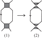
Figure 15. The trivial closed braid, arcs and bands.

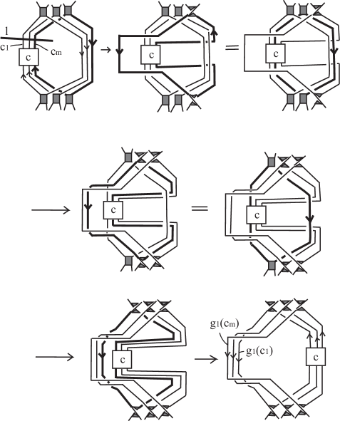
Figure 16. Deforming $S_{-1}$.

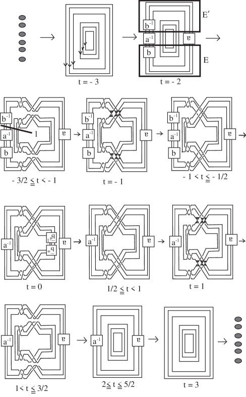
Figure 17. Motion picture of $S$ (5).

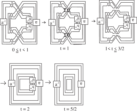
Figure 18. Motion picture of $S\cap\mathbb{R}^{3}[0,5/2]$ (6).

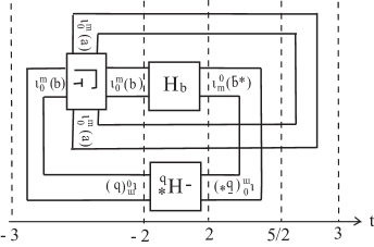
Figure 19. The $2m$-chart describing the surface braid $S_{\Gamma}$.

Step 4.  We will show that $S$ is equivalent to the surface link whose motion picture $\{S_{t}\}$ is as in Figure 17 for $t\in(-\infty,0)\cup(5/2,+\infty)$, and otherwise as in Figure 18. Further we will show that then $S$ is the closure of the required surface link $2m$-chart.

Let us consider a trivial closed 1-braid $\mathrm{cl}(e_{1})$ and two arcs in $\mathbb{R}^{3}$ with two untwisted bands connecting them as in Figure 15 (1). Let us take a 3-ball which contains $\mathrm{cl}(e_{1})$ and the bands. Then, by an ambient isotopy of $\mathbb{R}^{3}$ relative the complement of the 3-ball, we can deform $\mathrm{cl}(e_{1})$ and the bands to be as in Figure 15 (2).

Consider a neighborhood of $-\mathrm{cl}(\iota\bar{\Delta}\bar{\Delta}^{-1})\cup\mathcal{B}_{3}$ in $S_{-1}$ of Step 3 (see Figure 14). Since $-\mathrm{cl}(\iota\bar{\Delta}\bar{\Delta}^{-1})$ is equivalent to $-\mathrm{cl}(\iota e_{m})$, we can take $m$ disjoint 3-balls in $\mathbb{R}^{3}$ such that the intersection of $S_{-1}$ and each 3-ball is as in Figure 15 (1). Let $c_{j}$ be the $j$th string of $-\mathrm{cl}(\iota\bar{\Delta}\bar{\Delta}^{-1})$. Apply the deformation of Figure 15 to the 3-balls which contains $\mathrm{cl}(c_{1})$, $\mathrm{cl}(c_{2}),\ldots,\mathrm{cl}(c_{m})$ and the attaching bands in this order (see Figure 16, where we consider the case $c=e_{m}$). Let $\{g_{u}\}$ be the associated ambient isotopy. Since $c_{j-1}$ is over $c_{j}$ with respect to the $z$-axis, $g_{1}(c_{j})$ is over $g_{1}(c_{j-1})$ with respect to the $z$-axis ($j=2,3,\ldots,m$). Since $g_{1}(\iota\bar{\Delta})$ is the $m$-braid obtained from $\iota\bar{\Delta}$ by changing each crossing, for $\iota\bar{\Delta}$ with attaching bands, we have $g_{1}(\iota\bar{\Delta})=\iota\Delta$. Thus $g_{1}(\iota\bar{\Delta}\bar{\Delta}^{-1})=\iota\Delta\Delta^{-1}$. Further we can assume that $g_{1}(-\mathrm{cl}(\iota\bar{\Delta}\bar{\Delta}^{-1}))=\mathrm{cl}(\iota\Delta^{-1}\Delta\Delta^{-1}\Delta)$ as in Figure 16. Put $\mathcal{B}_{4}=g_{1}(\mathcal{B}_{3})$, which is a band set such that each band has one twist. Then $g_{1}(S_{-1})$ is a closed singular $2m$-braids such that the attaching band set $\mathcal{B}_{4}$ consists of $2m$ bands which correspond to the $m$ $\sigma_{m}$’s and $m$ $\sigma_{m}^{-1}$’s, connecting the inner closed $m$-braid and outer closed $m$-braid.

Let $E_{1}$ be a cylinder in $\mathbb{R}^{3}$ indicated at $t=-1/2$ in Figure 14. Note that $S_{-1/2}\cap E_{1}$ is the trivial $m$-braid. We can see that if we have an $m$-braid $c$ in $E_{1}$, then $g_{1}(c)=c$ in the cylinder $g_{1}(E_{1})$ (see Figure 16). Then by an ambient isotopy of (4.2) with $h_{u}=g_{u}$ and $t_{1}=-5$, $t_{2}=-4$, $t_{3}=4$, $t_{4}=5$, we can deform $S$ to have the motion picture as in Figure 17, as follows.

Let us denote by $e_{2m}$ the trivial $2m$-braid, and let $\tilde{\mathcal{D}}_{-,2m}$ (resp. $\tilde{\mathcal{D}}_{+,2m}$) be a trivial disk system of $2m$ components in $\mathbb{R}^{3}(-\infty,t]$ (resp. $\mathbb{R}^{3}[t,+\infty)$) with boundary $\mathrm{cl}(e_{2m})[t]$, where $t\in\mathbb{R}$. Let $\iota_{0}^{m}(\Gamma_{T})$ be the $2m$-chart obtained from the $m$-chart $\Gamma_{T}$ by adding $m$ trivial sheets after $\Gamma_{T}$, i.e. the $2m$-chart presented by $\Gamma_{T}$. And let $A(\iota_{0}^{m}(\Gamma_{T}))$ be the simple braided surface over an annulus associated with $\iota_{0}^{m}(\Gamma_{T})$. From now on, we denote by $\Delta$ (resp. $\Delta^{\prime}$) the $2m$-braid $\Delta_{m}$ (resp. $\Delta_{m}^{\prime}$). Further, we put $\Theta=\Theta_{m}$. Let us take $l$, which is indicated at $t=-3/2$ in Figure 17. Then the motion picture of $S$ is as follows (see Figure 17), where we take the identified corresponding ends of a closed braid in $l$ for $t\in[-3,\,3]$.

1. $S\cap\mathbb{R}^{3}(-\infty,-3]=\tilde{\mathcal{D}}_{-,2m}$. We have $S_{-3}=\mathrm{cl}(e_{2m})$.

2. $S\cap\mathbb{R}^{3}[-3,-2]=A(\iota_{0}^{m}(\Gamma_{T}))$. We have $S_{-2}=\mathrm{cl}(\iota_{0}^{m}(a^{-1}bab^{-1}))$.

3. $S_{-2}\rightarrow S_{-3/2}$ is an isotopic transformation such that

   $$S_{-3/2}=\mathrm{cl}(\iota^{m}_{0}(a^{-1}b)\cdot\Delta^{\prime-1}\Delta^{-1}\Delta^{\prime}\Delta\cdot\iota^{m}_{0}(a)\cdot\Delta^{-1}\Delta^{\prime-1}\Delta\Delta^{\prime}\cdot\iota^{m}_{0}(b^{-1})).$$

4. $S_{-3/2}\rightarrow S_{-1/2}$ is a hyperbolic transformation along the band set $\mathcal{B}_{4}\subset S_{-1}$. We have $S_{-1/2}=\mathrm{cl}(\iota^{m}_{0}(a^{-1}b)\cdot\Delta^{\prime-1}\Delta^{-1}\Theta\cdot\iota^{m}_{0}(a)\cdot\Theta^{-1}\Delta\Delta^{\prime}\cdot\iota^{m}_{0}(b^{-1}))$.

5. $S_{-1/2}\rightarrow S_{0}$ is an isotopic transformation such that

   $$S_{0}=\mathrm{cl}(\iota^{m}_{0}(a^{-1})\cdot\Delta^{\prime-1}\Delta^{-1}\Theta\cdot\iota^{m}_{0}(a)\cdot\iota_{m}^{0}(\bar{b}^{*}\bar{b}^{*-1})\cdot\Theta^{-1}\Delta\Delta^{\prime}).$$

6. $S_{0}\rightarrow S_{1/2}$ is an isotopic transformation such that

   $$S_{1/2}=\mathrm{cl}(\iota^{m}_{0}(a^{-1})\cdot\Delta^{\prime-1}\Delta^{-1}\Theta\cdot\iota^{m}_{0}(a)\cdot\Theta^{-1}\Delta\Delta^{\prime}).$$

7. $S_{1/2}\rightarrow S_{3/2}$ is a hyperbolic transformation along the band set $\mathcal{B}_{4}\subset S_{1}$. We have

   $$S_{3/2}=\mathrm{cl}(\iota^{m}_{0}(a^{-1})\cdot\Delta^{\prime-1}\Delta^{-1}\Delta^{\prime}\Delta\cdot\iota^{m}_{0}(a)\cdot\Delta^{-1}\Delta^{\prime-1}\Delta\Delta^{\prime}).$$

8. $S_{3/2}\rightarrow S_{2}$ is an isotopic transformation such that $S_{2}=\mathrm{cl}(\iota_{0}^{m}(a^{-1}a))$.

9. $S_{t}=S_{2}$ for $t\in[2,5/2]$.

10. $S_{5/2}\rightarrow S_{3}$ is an isotopic transformation such that $S_{3}=\mathrm{cl}(e_{2m})$.

11. $S\cap\mathbb{R}^{3}[3,+\infty)=\tilde{\mathcal{D}}_{+,2m}$.

Let us consider an ambient isotopy $\{H_{u}\}_{u\in[0,1]}$ of $\mathbb{R}^{3}[0,5/2]$ rel $\mathbb{R}^{3}[0]\cup\mathbb{R}^{3}[5/2]$ such that for each $u\in[0,1]$ and $\mathbf{x}\in\mathbb{R}^{3}$,

(4.3) $$H_{u}(\mathbf{x},t)=\begin{cases}\big{(}h_{2ut}^{-1}(\mathbf{x}),t\big{)}&\mathrm{if}\ t\in[0,1/2]\\ \big{(}h_{u}^{-1}(\mathbf{x}),t\big{)}&\mathrm{if}\ t\in[1/2,2]\\ \big{(}h_{2u(t-2)}\circ h_{u}^{-1}(\mathbf{x}),t\big{)}&\mathrm{if}\ t\in[2,5/2],\end{cases}$$

where $\{h_{u}\}_{u\in[0,1]}$ is the ambient isotopy of $\mathbb{R}^{3}$ such that $h_{u}(S_{0})=S_{u/2}$ for each $u$. By $\{H_{u}\}$, $S$ is equivalent to the surface link whose motion picture $\{S_{t}\}$ is as in Figure 17 for $t\in(-\infty,0)\cup(5/2,\infty)$, and otherwise as follows (see Figure 18).

1. $S_{t}=S_{0}=\mathrm{cl}(\iota^{m}_{0}(a^{-1})\cdot\Delta^{\prime-1}\Delta^{-1}\Theta\cdot\iota^{m}_{0}(a)\cdot\iota^{0}_{m}(\bar{b}^{*}\bar{b}^{*-1})\cdot\Theta^{-1}\Delta\Delta^{\prime})$ for $t\in[0,1/2]$.

2. $S_{1/2}\rightarrow S_{3/2}$ is a hyperbolic transformation along the band set $\mathcal{B}_{4}\subset S_{1}$. We have

   $$S_{3/2}=\mathrm{cl}(\iota^{m}_{0}(a^{-1})\cdot\Delta^{\prime-1}\Delta^{-1}\Delta^{\prime}\Delta\cdot\iota^{m}_{0}(a)\cdot\iota^{0}_{m}(\bar{b}^{*}\bar{b}^{*-1})\cdot\Delta^{-1}\Delta^{\prime-1}\Delta\Delta^{\prime}).$$

3. $S_{3/2}\rightarrow S_{2}$ is an isotopic transformation such that

   $$S_{2}=\mathrm{cl}(\iota_{0}^{m}(a^{-1}a)\cdot\iota_{m}^{0}(\bar{b}^{*}\bar{b}^{*-1})).$$

4. $S_{2}\rightarrow S_{5/2}$ is an isotopic transformation such that $S_{5/2}=\mathrm{cl}(\iota_{0}^{m}(a^{-1}a))$.

Note that the band set $\mathcal{B}_{4}$ consists of $2m$ bands which correspond to the $m$ $\sigma_{m}$’s and $m$ $\sigma_{m}^{-1}$’s, connecting the inner and outer closed $m$-braids.

The figures describing the motion pictures of $S$ are for the case $m=3$. However, since each step can be applied for an arbitrary positive integer $m$, we can regard them as describing the motion pictures of $S$ for arbitrary $m$. Now, the motion picture $\{S_{t}\}$ of $S$ is as in Figure 17 for $t\in(-\infty,0)\cup(5/2,+\infty)$, and otherwise as in Figure 18. Thus $S$ is the closure of the surface braid obtained from $S\cap\mathbb{R}^{3}[-3,3]$ by cutting it along $l[-3,3]$. Let us denote the surface braid by $S_{\Gamma}$. Let us take cylinders $E$ and $E^{\prime}$ in $\mathbb{R}^{3}$ such that the closed $2m$-braid $S_{t}$ is presented by $\iota_{0}^{m}(a^{-1})\cdot(S_{t}\cap E)\cdot\iota_{0}^{m}(a)\cdot(S_{t}\cap E^{\prime})$ for $t\in[-2,2]$, where $S_{t}\cap E$ and $S_{t}\cap E^{\prime}$ are classical $2m$-braids; see the figure at $t=-2$ in Figure 17. Then $S_{\Gamma}\cap(E[-2,2])$ is a braided surface of degree $2m$ such that

1. $S_{-2}\cap E=\iota_{0}^{m}(b)$,

2. $S_{-2}\cap E\rightarrow S_{-3/2}\cap E$ is an isotopic transformation such that $S_{-3/2}\cap E=\iota_{0}^{m}(b)\cdot\Delta^{\prime-1}\Delta^{-1}\Delta^{\prime}\Delta$.

3. $S_{-3/2}\cap E\rightarrow S_{-1/2}\cap E$ is a hyperbolic transformation along a band set which consists of $m$ bands corresponding to the $m$ $\sigma_{m}$’s. We have $S_{-1/2}\cap E=\iota_{0}^{m}(b)\cdot\Delta^{\prime-1}\Delta^{-1}\Theta$.

4. $S_{-1/2}\cap E\rightarrow S_{0}\cap E$ is an isotopic transformation such that $S_{0}\cap E=\Delta^{\prime-1}\Delta^{-1}\Theta\cdot\iota_{m}^{0}(\bar{b}^{*})$.

5. $S_{0}\cap E\rightarrow S_{3/2}\cap E$ is a hyperbolic transformation along a band set which consists of $m$ bands corresponding to the $m$ $\sigma_{m}$’s. We have $S_{3/2}\cap E=\Delta^{\prime-1}\Delta^{-1}\Delta^{\prime}\Delta\cdot\iota_{m}^{0}(\bar{b}^{*})$.

6. $S_{3/2}\cap E\rightarrow S_{2}\cap E$ is an isotopic transformation such that $S_{2}\cap E=\iota_{m}^{0}(\bar{b}^{*})$.

Thus the braided surface $S_{\Gamma}\cap E[-2,2]$ is presented by the 1-handle $2m$-chart $H_{b}$. If $a$ is the trivial $m$-braid, then $S\cap\mathbb{R}^{3}[t]$ is equivalent to the trivial closed $2m$-braid for $t\in[-2,2]-\{-1,1\}$. Thus $(S_{t}\cap E)\cdot(S_{t}\cap E^{\prime})=e_{2m}$, and hence

(4.4) $$S_{t}\cap E^{\prime}=(S_{t}\cap E)^{-1}$$

for $t\in[-2,2]-\{-1,1\}$. Further, $S_{-1}\cap E^{\prime}$ and $S_{1}\cap E^{\prime}$ are singular classical $2m$-braids such that the singular points are presented by $m$-bands corresponding to $m$ $\sigma_{m}^{-1}$’s. Let us consider a $2m$-chart $\Gamma$. Let $\rho$ be a path which intersects with the edges of $\Gamma$ transversely. Let $c=\sigma_{i_{1}}^{\epsilon_{i_{1}}}\sigma_{i_{2}}^{\epsilon_{i_{2}}}\cdots\sigma_{i_{\nu}}^{\epsilon_{i_{\nu}}}$ be the $2m$-braid presented by $\rho\cap\Gamma$. Let us consider the orientation-reversed mirror image of $\Gamma$ and $\rho$, and denote it by $-\Gamma^{*}$ and $-\rho^{*}$ respectively. Then $-\rho^{*}\cap(-\Gamma^{*})$ presents $\sigma_{i_{\nu}}^{-\epsilon_{i_{\nu}}}\sigma_{i_{\nu-1}}^{-\epsilon_{i_{\nu-1}}}\cdots\sigma_{i_{1}}^{-\epsilon_{i_{1}}}$, which is $c^{-1}$. Hence, by (4.4) we can see that $S_{\Gamma}\cap(E^{\prime}[-2,2])$ is the braided surface presented by a $2m$-chart $f(-H_{b}^{*})$, where $-H_{b}^{*}$ is the orientation-reversed mirror image of $H_{b}$ and $f$ is the map which rotates $-H_{b}^{*}$ by $\pi$. More precisely, assuming that $-H_{b}^{*}$ is on a 2-disk $[-1,1]\times[-1,1]$, $f$ is a self-homeomorphism of the 2-disk defined by $f(t_{1},t_{2})=-(t_{1},t_{2})$. Thus the surface braid $S_{\Gamma}$ is presented by the surface link $2m$-chart as in Figure 19. Since the $2m$-chart can be taken to be as in Figure 4 by an ambient isotopy, $S$ is presented by the required $2m$-chart. ∎

An orientable surface link $F$ is trivial (or unknotted) if there is an embedded 3-manifold $M$ with $\partial M=F$ such that each component of $M$ is a handlebody. An oriented surface link is called ribbon if it is obtained from a trivial 2-link $F_{0}$ by 1-handle surgeries along a finite number of mutually disjoint 1-handles attaching to $F_{0}$.

Kamada showed [8] that surface links whose braid index is at most three are indeed ribbon, and Shima showed [18] that the turned spun $T^{2}$-knot of a non-trivial classical knot is not ribbon. Hence we obtain the following corollary.

Corollary 4.1.

Let $S$ be the torus-covering link presented by a torus-covering $m$-chart. Then the braid index of S is equal or less than $2m$. In particular, the braid index of the turned spun $T^{2}$-knot of the torus $(2,\,p)$-knot is four.

Remark 4.2.

Hasegawa [6, Part 3 “Chart description of twist-spun surface-links”] showed that for the turned spun $T^{2}$-link of a closed $m$-braid, its braid index is at most $3m$.

5. Example

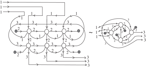
Figure 20. The 1-handle $4$-chart $H_{b}$, where $b=\sigma_{1}^{3}$.

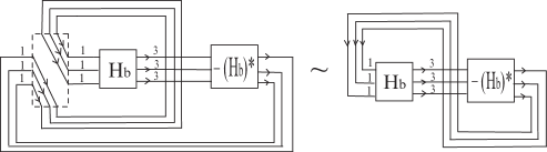
Figure 21. The surface link $4$-chart $\Gamma_{S}$ obtained from $\Gamma_{T}$.

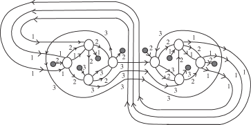
Figure 22. The surface link $4$-chart $\Gamma_{S}$.

Let us consider the torus-covering $2$-chart $\Gamma_{T}$ of Example 2.4 (2), that is, the torus-covering $2$-chart $\Gamma_{T}$ of Figure 3 (2). The torus-covering link $S$ associated with $\Gamma_{T}$ is the turned spun $T^{2}$-knot of the right-handed trefoil. In the notations of Theorem 3.2, we have $a=b=\sigma_{1}^{3}$. By the theorem, the 1-handle $4$-chart $H_{b}$ is as in the left figure of Figure 20. It is $C$-move equivalent to the right figure of Figure 20. Thus the surface link $4$-chart $\Gamma_{S}$ on a 2-disk obtained from $\Gamma_{T}$ is as in the left figure of Figure 21. It is equivalent to the right figure of Figure 21 by an ambient isotopy of the 2-disk. Thus $\Gamma_{S}$ is as in Figure 22.

Acknowledgements. The author would like to thank Professors Takashi Tsuboi and Elmar Vogt for suggesting this topic, and Professors Akio Kawauchi, Tomotada Ohtsuki, and the referee for their valuable advice.

References

- [1] J. Birman, Braids, links, and mapping class groups, Ann. Math. Studies 82 (Princeton Univ. Press, Princeton, N.J., 1974).
- [2] J. Boyle, Classifying 1-handles attached to knotted surfaces, Trans. Amer. Math. Soc. 306 (2) (1988), 475–487.
- [3] J. Boyle, The turned torus knot in , J. Knot Theory Ramifications 2 (1993) 239–249.
- [4] J. S. Carter and M. Saito, Knotted surfaces and their diagrams, Mathematical Surveys and Monographs 55 (Amer. Math. Soc., 1998).
- [5] F. A. Garside, The braid group and other groups, Quart. J. Math. Oxford (2) 20 (1969) 235–254.
- [6] I. Hasegawa, Chart descriptions of monodromy representations on oriented closed surfaces, Ph. D. Thesis, the University of Tokyo (2005).
- [7] Z. Iwase, Dehn-surgery along a torus -knot, Pacific J. Math. 133 (1988) 289–299.
- [8] S. Kamada, Surfaces in of braid index three are ribbon, J. Knot Theory Ramifications 1 No.2 (1992) 137–160.
- [9] S. Kamada, 2-dimensional braids and chart descriptions, “Topics in Knot Theory (Erzurum, 1992)”, 277–287, NATO Adv. Sci. Inst. Ser. C Math. Phys. Sci., 399, Kluwer Acad. Publ., (Dordrecht, 1993).
- [10] S. Kamada, A characterization of groups of closed orientable surfaces in 4-space, Topology 33 (1994) 113-122.
- [11] S. Kamada, An observation of surface braids via chart description, J. Knot Theory Ramifications 4 (1996) 517–529.
- [12] S. Kamada, Braid and Knot Theory in Dimension Four, Math. Surveys and Monographs 95 (Amer. Math. Soc., 2002).
- [13] A. Kawauchi, On pseudo-ribbon surface-links, J. Knot Theory Ramifications 11 No.7 (2002) 1043–1062.
- [14] C. Livingston, Stably irreducible surfaces in , Pacific J. Math. 116 (1985), 77–84.
- [15] I. Nakamura, Surface links which are coverings over the standard torus, Algebraic and Geometric Topology 11 (2011), 1497–1540.
- [16] C. P. Rourke and B. J. Sanderson, Introduction to piecewise-linear topology, (Springer-Verlag, 1972).
- [17] L. Rudolph, Braided surfaces and Seifert ribbons for closed braids, Comment. Math. Helv. 58 no.1 (1983), 1–37.
- [18] A. Shima, Knotted Klein bottles with only double points, Osaka J. Math. 40 (2003) 779–799.
- [19] M. Teragaito, Symmetry-spun tori in the four sphere, in Knots 90, pp. 163–171.