Phase transitions and localizable entanglement in cluster-state spin chains
with Ising couplings and local fields

Abstract

We consider a one-dimensional spin chain for which the ground state is the cluster state, capable of functioning as a quantum computational wire when subjected to local adaptive measurements of individual qubits, and investigate the robustness of this property to local and coupled (Ising-type) perturbations. We investigate the ground state both by identifying suitable correlation functions as order parameters, as well as numerically using a variational method based on matrix product states. We find that the model retains an infinite localizable entanglement length for Ising and local fields up to a quantum phase transition, but that the resulting entangled state is not simply characterized by a Pauli correction based on the measurement results.

I Introduction

Measurement-based quantum computation (MBQC) Briegel et al. (2009) has recently emerged as an alternative model for quantum computation to the standard circuit model Nielsen and Chuang (2000). In MBQC, computation proceeds via local (single-qubit) adaptive measurements on a fixed fiducial state of a quantum many-body system, for which the cluster state Briegel et al. (2009); Raussendorf et al. (2003) is the canonical example.

The MBQC model of quantum computation is particularly useful for investigating the physical requirements for quantum computing, as it becomes possible to pose questions about universality and fault-tolerance in terms of properties of quantum states Raussendorf et al. (2005, 2007); Gross and Eisert (2007); Gross et al. (2007); van den Nest et al. (2007); Brennen and Miyake (2008); Doherty and Bartlett (2008); Barrett et al. (2008); Gross et al. (2009); Bremner et al. (2009). For example, the universality of a given quantum state for MBQC may be determined by assessing the fidelity and range of a universal quantum gate set, which in turn is quantified by viewing gates as resource states for gate teleportation Gottesman and Chuang (1999); Raussendorf et al. (2003) prepared via local measurements Chung et al. (2009).

However, despite this powerful framework, there are relatively few known examples of resources states (or distinct classes of states) that allow for MBQC Gross and Eisert (2007); Gross et al. (2007); van den Nest et al. (2007). A promising avenue for identifying properties of states that allow for MBQC is by investigating ground or low-temperature thermal states of a coupled quantum many-body system Bartlett and Rudolph (2006); Griffin and Bartlett (2008); Brennen and Miyake (2008). In particular, one can construct model Hamiltonians for which the ground state is universal for MBQC (say, the cluster state on some appropriate lattice) and then investigate the robustness of this property to local perturbations. Progress has been made in this direction for thermal or local perturbations of the cluster state Raussendorf et al. (2005); Doherty and Bartlett (2008); Barrett et al. (2008).

In this paper, we investigate a 1D chain of qubits for which the cluster state is the ground state, and investigate the robustness of its computational power to both local and coupled (Ising-type) perturbations. (For a 1D chain, “computational power” is restricted to single-qubit unitary evolution.) Consistent with previous results Doherty and Bartlett (2008); Barrett et al. (2008), we identify a robust phase for which every ground state can allow for quantum information to be transferred using local measurements. We investigate the usefulness for states in this phase to serve as “quantum computational wires” Gross and Eisert (2008), which function as primitives for MBQC.

I.1 Quantum computational wires

Within MBQC, the simplest primitive is the ability to move information (i.e., teleport) along one-dimensional channels, with single-qubit unitaries determined by the choice of measurements. States with this property are known as quantum computational wires Gross and Eisert (2008). A wire in MBQC consists of two parts: (i) creating a maximally-entangled state between two distant points via local measurements; and (ii) identifying the correct “bi-product” unitary based on the measurement result (either to implement the identity gate, or some more general single-qubit unitary gate). The first property is characterized by localizable entanglement Popp et al. (2005), which is the maximum average entanglement that can be localized on two sites through local measurements on all other sites. For systems where the localizable entanglement falls of exponentially, the entanglement length $\xi_{E}$ is defined through

$$E_{L}\sim e^{-n/\xi_{E}}\qquad\text{when }n\gg 1\,,$$ (1)

with $n$ the separation between the sites; states with finite localizable EL are not directly useable as a quantum computational wire. In contrast, systems with infinite localizable EL allow for teleportation over arbitrary length scales. One of the characteristics of the cluster state is a diverging localizable EL. (We note, however, that diverging EL is in itself not necessary nor sufficient for the state to be useful for MBQC Gross and Eisert (2007).)

In general, identifying an optimal measurement basis for localizing entanglement can be a challenge. For the cluster state on any lattice, such an optimal measurement strategy is known: measure $Z$ (i.e., measure in the eigenbasis of $\sigma^{z}$) on all qubits except those on a line connecting the two desired qubits, thus effectively making a 1D cluster state, and then measure $X$ on all intermediate qubits along the remaining line. This measurement sequence will concentrate a maximally-entangled state on the two remaining qubits.

To transform the resulting maximally-entangled state into a particular one (say, the two-qubit cluster state), a correction unitary on one of the qubits based on the measurement results is then applied. If these corrections are Pauli operations, or in general if they close to form a finite subgroup, then the bi-product operators do not need to be performed but instead one can use a classical computer to keep track of them. In general, however, even if the localizable EL is infinite, the bi-product operators may not close in this way. That is, there is a distinction between infinite localizable EL and the ability to function as a quantum computational wire.

This paper is structured as follows. In Sec. II, we introduce our Hamiltonian with local and coupled perturbations, and investigate its phase diagram. Here, we identify a cluster phase connected to the cluster state (with zero perturbations). We consider using correlation functions as for the cluster state to quantify the identity gate within the cluster phase in Sec. III. In Sec. IV, we use numerical methods to assess the localizable entanglement within our model, and in Sec. V we investigate the usefulness of ground states in the cluster phase to serve as a quantum computational wire. In Sec. VI we turn our attention to the use of local measurements to disentangle the two halves of the chain, in analogy to the $Z$ measurement in cluster state MBQC, and finish with conclusions in Sec. VII. The appendix provides details on the Jordan-Wigner transformation.

II Cluster Hamiltonian with anomalous terms

II.1 The cluster state and cluster Hamiltonian

Consider a graph (such as a lattice) containing $N$ vertices, with a qubit placed on each vertex. The cluster state on this graph can be constructed by first preparing each qubit in the state $|+\rangle$, the $+1$ eigenstate of the $\sigma^{x}$ Pauli spin operator, and then applying a controlled sign operator $U=\exp(i\pi|1\rangle\langle 1|\otimes|1\rangle\langle 1|)$ on every pair of qubits on vertices connected by an edge. The resulting cluster state is compactly described in terms of stabilizers. That is, at every vertex $\mu=1,\ldots,N$ one associates an operator

$$K_{\mu}=\sigma^{x}_{\mu}\prod_{\nu\sim\mu}\sigma^{z}_{\nu}\,,$$ (2)

where $\nu\sim\mu$ indicates all vertices $\nu$ that are connected to $\mu$. In a graph of degree $\chi$, this operator acts on $\chi+1$ vertices. The cluster state is the unique state $|C\rangle$ that satisfies

$$K_{\mu}|C\rangle=|C\rangle\,,\qquad\forall\ \mu\,.$$ (3)

An alternate approach to prepare a cluster state would be to view the qubits on this graph as an interacting quantum many-body system, and to find some Hamiltonian $H_{C}$ for which the cluster state is the unique ground state. Provided the model has a sufficiently large gap, preparation of the state would amount to cooling the system down to (or near) the ground state. One such Hamiltonian that has the cluster state as its ground state is (minus) the sum of the stabilizers at every site $\mu$ Raussendorf et al. (2005),

$$H_{C}=-\sum_{\mu}K_{\mu}\,.$$ (4)

We have chosen units such that the energy scale is fixed, and the gap in the model is 2 between the unique ground state and a $N$-fold degenerate first excited state. Although the terms $K_{\mu}$ is this Hamiltonian are generally many-body, such interactions can occur as the low-energy behavior of a more natural two-body Hamiltonian Bartlett and Rudolph (2006); Griffin and Bartlett (2008). We note that the cluster state on a line – the ground state of the Hamiltonian (4) – has an infinite localizable EL and can serve as a quantum computational wire. This Hamiltonian on a line can be realized in an optical lattice despite its three-body interactions Pachos and Plenio (2004).

II.2 Cluster Hamiltonian with anomalous terms

Consider the cluster state Hamiltonian (4) in one dimension with two types of additional terms: local fields and couplings,

$$H=H_{C}-\sum_{\mu}\vec{B}\cdot\vec{\sigma}_{\mu}-J\sum_{\mu}\sigma^{z}_{\mu}\sigma^{z}_{\mu+1}\,,$$ (5)

with $J\geq 0$. Unless otherwise specified, we will consider periodic boundary conditions, such that $\vec{\sigma}_{N+1}=\vec{\sigma}_{1}$. Throughout the article we will restrict our attention to $B_{y}=0$.

(Note that an Ising interaction as in the last term of Eq. (5) can be used in a time modulated fashion to construct a cluster state Raussendorf et al. (2003). However, we will study this term only as a constant perturbation of the Hamiltonian.)

A number of results are known for specific cases involving a single local term and $J=0$:

Local $B_{z}$ field: In one dimension, the system is fundamentally unstable with the addition of a local $z$ field, i.e., the EL becomes finite for any non-zero $B_{z}$. In two- or higher-dimensional lattices, however, it can be shown using techniques from percolation theory that the model exhibits a transition from a finite region of parameter space $B_{z}<B_{z}^{\rm crit}$ wherein the ground state has infinite localizable EL. Because the localizable EL is zero in the limit $B_{z}\to\infty$, there is a transition in the localizable EL for two- or higher-dimensional lattices even though the underlying model does not exhibit any quantum phase transition Barrett et al. (2008).

Local $B_{x}$ field: In one dimension, the system exhibits a single quantum phase transition at $B_{x}=1$ separating the “cluster phase” and a separable phase. Ground states in the cluster phase are characterized by infinite localizable EL Pachos and Plenio (2004); Doherty and Bartlett (2008), and the system serves as a quantum computational wire at all length scales (with precisely the same measurement sequence and corrections as for the cluster state) albeit with lower fidelity for all $B_{x}<1$. The performance as a quantum computational wire is therefore a robust property of this system in the presence of a perturbing $B_{x}$ field.

With these prior results, we now analyze the full phase space of the Hamiltonian (5). Consider the action on this model of the unitary transformation $\mathbf{U}=\prod_{\mu\nu}U_{\mu\nu}$ that applies the controlled phase gate $U_{\mu\nu}$ on all pairs of adjacent qubits. This unitary maps $H_{C}$ to

$$\mathbf{U}H_{C}\mathbf{U}^{\dagger}=-\sum_{\mu}\sigma_{\mu}^{x}\,,$$ (6)

for which the ground state is separable, $\mathbf{U}|C\rangle=|+\rangle^{\otimes N}$. In general, the transformation leaves $\sigma^{z}$ operators invariant, while $\sigma^{x}$ maps to

$$\mathbf{U}\sigma^{x}_{\mu}\mathbf{U}^{\dagger}=\sigma^{x}_{\mu}\prod_{\nu\sim\mu}\sigma^{z}_{\nu}=K_{\mu}\,.$$ (7)

This transformation allows us to determine some properties of the model (5). First, consider the model with $\vec{B}=0$. Under this unitary mapping, the model is dual to the ordinary transverse-field Ising model, which is completely solved in 1D Pfeuty (1970), and has a single quantum phase transition at $J=1$. For our model (5) in the large $J$ limit with $\vec{B}=0$, the ground state approaches a GHZ state

$$|GHZ\rangle=\frac{1}{\sqrt{2}}\left(|00\cdots 0\rangle+|11\cdots 1\rangle\right)\,.$$ (8)

We denote the phase for $J>1$ the Ising phase.

From the local $B_{z}$ results, we do not expect the properties of the cluster state to survive for any $B_{z}>0$, and so we now consider the restricted model with $B_{z}=0$. This model can be subjected to a Jordan-Wigner transform as shown in Appendix A, which easily allows identification of critical points in the model, and hence diverging correlation and entanglement lengths. This restricted model has three clearly identifiable phases: the cluster phase as $B_{x},J\to 0$, an Ising phase as $J\gg\max(1,B_{x})$ and a separable phase as $B_{x}\gg\max(1,J)$. The model is unitarily dual under the transformation $\mathbf{U}$. Thus, for any critical point at $(J,B_{x})$, there is another critical point at $(\frac{J}{B_{x}},\frac{1}{B_{x}})$. Thus, considering the critical line $\mathcal{C}_{C}$ connecting the known critical points at $(0,1)$ and $(1,0)$, this duality reveals another critical line $\mathcal{C}_{G}$ from $(0,1)$ to $(\infty,\infty)$. Parameterizing the lines with a parameter $\tau\in[0,1]$, we have

$$\mathcal{C}_{C}=(\tau,f(\tau))\qquad\mathcal{C}_{G}=\left(\frac{\tau}{f(\tau)},\frac{1}{f(\tau)}\right)\,,$$ (9)

for some unknown function $f(\tau)$, for which $f(0)=1$ and $f(1)=0$. In the limit $B_{x},J\gg 1$, the cluster term in the Hamiltonian becomes unimportant, and the model is a simple Ising model for which the critical point must be at $B_{x}=J$. Under the above parameterization we must have, assuming $f(\tau)$ is continuous, and invoking l’Hôpital’s rule,

$$\lim_{\tau\to 1}\frac{\tau}{f(\tau)}-\frac{1}{f(\tau)}=\lim_{\tau\to 1}\frac{\tau-1}{f(\tau)}=\lim_{\tau\to 1}\frac{1}{df/d\tau}=0\,,$$ (10)

which implies $\frac{df}{d\tau}=\infty$. Hence, the critical line $\mathcal{C}_{C}$ must be convex (at least close to $J=1$). The numerical results indicate that this convergence is very slow, and to a close approximation we have $f(\tau)=1-\tau$, and hence $\mathcal{C}_{G}=(\tau^{\prime},1+\tau^{\prime})$, $\tau^{\prime}\in[0,\infty]$. The three phases are separated by Ising type critical lines corresponding to a conformal field theory with central charge $c=1/2$, and a corresponding entanglement signature Skrøvseth and Olaussen (2005).

In the phase diagram of Fig. 1 for $B_{z}=0$, at the origin ($J=B_{x}=0$) the ground state is the cluster state. From the results of Pachos and Plenio (2004); Doherty and Bartlett (2008), we know that ground states on the line $J=0$, $0\leq B_{x}<1$ have infinite localizable EL, and in fact allow for long-ranged single-qubit gates using the same measurement sequence and Pauli corrections as for the cluster state. We now turn our attention to the question: is any ground state within the cluster phase of Fig. 1 also useful as such a quantum computational wire?

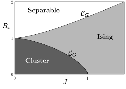
Figure 1: A sketch of the phase diagram for the Hamiltonian in Eq. (5) with $B_{z}=0$. The lines $\mathcal{C}_{G}$ and $\mathcal{C}_{C}$ constitute quantum phase transitions between the three indicated phases. (All quantities shown in figures in this paper, including this one, are dimensionless.)

III Correlation functions for localizable entanglement and quantum computational wires

In special cases, the localizable entanglement of a state can be characterized (or, at least, lower bounded) by a correlation function. For example, with certain measurement sequences, one can obtain post-measurement quantities from pre-measurement expectation values to quantify the localizable entanglement Verstraete et al. (2004a); Popp et al. (2005); Venuti and Roncaglia (2005) or the performance of quantum gates in MBQC Chung et al. (2009); Doherty and Bartlett (2008). That is, the expectation values of string-like operators can serve as order parameters to identify the hidden correlations corresponding to localizable entanglement and the ability to function as a quantum computational wire.

III.1 Localizable entanglement for $B_{z}=0$

For $B_{z}=0$, the symmetries of our model allow us to determine the optimal measurement sequence and to derive an expression for the localizable entanglement Verstraete et al. (2004a); Popp et al. (2005); Venuti and Roncaglia (2005). Our model (5) with $B_{z}=0$ is invariant under rotations of all spins by $\pi$ about the $x$ axis, transforming $\sigma^{z}\rightarrow-\sigma^{z}$. It is not invariant under similar rotations about the $y$ and $z$ axes; therefore, the optimal measurements for localizing entanglement on a finite chain between the end qubits $1$ and $N$ are measurements in the $X$-basis Verstraete et al. (2004a); Popp et al. (2005); Venuti and Roncaglia (2005). With this basis, the localizable entanglement for this finite chain is given by the string correlation function

$$E_{L}=\langle\sigma^{y}_{1}\Bigl{(}{\textstyle\prod_{j=2}^{N-1}}\sigma^{x}_{j}\Bigr{)}\sigma^{y}_{N}\rangle\,.$$ (11)

(We note that, for a suitable choice of boundary conditions on this finite chain, we could ensure that the ground state is a $+1$ eigenstate of $P^{x}=\prod_{j=1}^{N}\sigma^{x}_{j}$ and simplify this correlation function further. However, as we will be interested in open chains or periodic boundary conditions, we will not do so.)

This correlation function quantifies the localizable entanglement, but does not completely characterize the form of the resulting maximally entangled state. We now turn to a complete set of correlation functions for this, which quantify the state’s use as a quantum computational wire.

III.2 Correlation functions for quantum computational wires

In this section, we briefly summarize the main result of Ref. Chung et al. (2009). Consider a lattice of qubits prepared in some initial pure state $|\psi_{0}\rangle$. Singling out two qubits, $a$ and $b$, we consider a measurement sequence on the remaining qubits in the lattice that localizes entanglement on $a$ and $b$. Let $m$ label the measurement outcomes, and $P_{m}$ be the corresponding projector. Following the measurements, a correction unitary $U_{m}$ conditional on $m$ is applied to qubit $b$. Averaged over all possible measurement outcomes, the resulting two-qubit state is

$$\rho_{ab}={\textstyle\sum_{m}}U_{m}P_{m}|\psi_{0}\rangle\langle\psi_{0}|P_{m}U_{m}^{\dagger}\,.$$ (12)

Equivalently, we can characterize this final state using the set of expectation values of bipartite Pauli operators $\sigma^{i}_{a}\otimes\sigma^{j}_{b}$, $i,j=I,x,y,z$ on qubits $a$ and $b$, as

$$\langle\sigma^{i}_{a}\sigma^{j}_{b}\rangle_{\mathcal{P}} ={\textstyle\sum_{m}}\langle\psi_{0}|P_{m}U_{m}^{\dagger}\sigma^{i}_{a}\sigma^{j}_{b}U_{m}P_{m}|\psi_{0}\rangle$$

$$={\textstyle\sum_{m}}\langle\psi_{0}|P_{m}\sigma^{i}_{a}(\sigma^{j}_{b})_{m}P_{m}|\psi_{0}\rangle\,,$$ (13)

where $(\sigma^{j}_{b})_{m}=U_{m}^{\dagger}\sigma^{j}_{b}U_{m}$, and where $\langle\cdot\rangle_{\mathcal{P}}$ denotes the expectation value in the final post-measurement two-qubit state. The set of such correlation functions for all pairs of Pauli operators will completely specify the two-qubit state.

We now restrict our attention to measurement sequences for which there exists a string of operators $S$ acting on some set of the measured qubits which is independent of the measurement outcomes, and an operator $\tau^{j}_{b}$ on $b$ that is also independent of $m$, such that

$$\sigma^{i}_{a}(\sigma^{j}_{b})_{m}P_{m}=P_{m}\sigma^{i}_{a}S\tau^{j}_{b}\,.$$ (14)

For example, in the cluster state model of MBQC Raussendorf et al. (2003), a universal gate set is known that satisfies this property Chung et al. (2009). For such measurement sequences, using the projector properties $P_{m}^{2}=P_{m}$ and $\sum_{m}P_{m}=I$ gives

$$\langle\sigma^{i}_{a}\sigma^{j}_{b}\rangle_{\mathcal{P}}=\langle\psi_{0}|\sigma^{i}_{a}S\tau^{j}_{b}|\psi_{0}\rangle\,.$$ (15)

Thus we can relate the two-qubit state prepared after the sequence of measurements to a correlation function of the original state $|\psi_{0}\rangle$ prior to measurements. That is, the correlation functions characterize the post-measurement two-qubit state using expectation values of strings of operators on the pre-measurement state.

It is critical to this development that one can identify such a string of operators $S$. The measurement sequence for localizing entanglement in the cluster state provides the canonical example. For a $N$-qubit chain with $N$ even, using the same measurement sequence as if localizing entanglement in the cluster state $|C\rangle$ (measure $Z$ on qubits 1 and $N$, and $X$ on all qubits $3\cdots N-2$) with the same Pauli corrections as for the cluster state, the averaged state on qubits $a=2$ and $b=N-1$ afterwards has the following non-zero correlation functions:

$$\langle\sigma^{z}_{a}\sigma^{x}_{b}\rangle_{\mathcal{P}} =\langle C|\sigma^{z}_{2}\Bigl{(}{\textstyle\prod_{j=1}^{N/2-1}}\sigma^{x}_{2j+1}\Bigr{)}\sigma^{z}_{N}|C\rangle$$ (16a)

$$\langle\sigma^{x}_{a}\sigma^{z}_{b}\rangle_{\mathcal{P}} =\langle C|\sigma^{z}_{1}\Bigl{(}{\textstyle\prod_{j=1}^{N/2-1}}\sigma^{x}_{2j}\Bigr{)}\sigma^{z}_{N-1}|C\rangle$$ (16b)

$$\langle\sigma^{y}_{a}\sigma^{y}_{b}\rangle_{\mathcal{P}} =\langle C|\sigma^{z}_{1}\Bigl{(}{\textstyle\prod_{j=2}^{N-1}}\sigma^{x}_{j}\Bigr{)}\sigma^{z}_{N}|C\rangle$$ (16c)

Note that a two qubit cluster state has expectation values $\langle\sigma^{x}_{a}\sigma^{z}_{b}\rangle=\langle\sigma^{z}_{a}\sigma^{x}_{b}\rangle=\langle\sigma^{y}_{a}\sigma^{y}_{b}\rangle=1$, which means that the above expectation values are maximal for the cluster state.

III.3 Correlation functions for $B_{z}=0$

For our model (5) with $B_{z}=0$, the correlation functions of Eq. (16) can be calculated analytically using the exact solution obtained via the Jordan-Wigner transformation. In the cluster phase, of the three correlation functions given in Eq. (16), we find that only the expectation value $\langle\sigma^{y}_{a}\sigma^{y}_{b}\rangle_{\mathcal{P}}$ of Eq. (16c) remains long-ranged in the thermodynamic limit. This expectation value takes the general form of a transverse-field Ising order parameter. The other expectation values, $\langle\sigma^{z}_{a}\sigma^{x}_{b}\rangle_{\mathcal{P}}$ and $\langle\sigma^{x}_{a}\sigma^{z}_{b}\rangle_{\mathcal{P}}$, remain nonzero only for $J=0$. (As shown in Doherty and Bartlett (2008), for $J=0$ they remain long-ranged for $B_{x}<1$.) Fig. 2 shows the behaviour of these expectation values for the ground state of the model with $\vec{B}=0$.

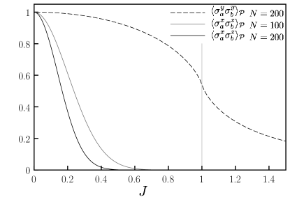
Figure 2: Expectation values $\langle\sigma^{x}_{a}\sigma^{z}_{b}\rangle_{\mathcal{P}}$ and $\langle\sigma^{y}_{a}\sigma^{y}_{b}\rangle_{\mathcal{P}}$ for $B_{x}=B_{z}=0$. The former is shown for $N=100,200$ while $\langle\sigma^{y}_{a}\sigma^{y}_{b}\rangle_{\mathcal{P}}$ is shown for $N=200$ only, as this is not size dependent, and indistinguishable from $N=100$. The expectation value $\langle\sigma^{z}_{a}\sigma^{x}_{b}\rangle_{\mathcal{P}}$ is identical to $\langle\sigma^{x}_{a}\sigma^{z}_{b}\rangle_{\mathcal{P}}$.

The long-ranged behaviour of $\langle\sigma^{y}_{a}\sigma^{y}_{b}\rangle_{\mathcal{P}}$ in the cluster phase serves as a useful order parameter, and is related to the expression for the finite-chain localizable entanglement of Eq. (11). However, the fact that the other correlation functions of Eq. (16) are zero for $J>0$ shows that the standard cluster-state Pauli corrections based on the measurement results are not suitable, i.e., the resulting bipartite state is not the two-qubit cluster state. We now turn to numerical methods to investigate the exact form of the resulting bipartite entangled state in the cluster phase.

IV Numerical calculations using matrix product states

Our analytic approach to investigating the cluster phase has identified an appropriate order parameter for the localizable entanglement, realized as the expectation value of a string operator, but has not revealed the form of the resulting bipartite entangled state necessary for use as a quantum computational wire. We now use numerical methods based on Matrix Product States to investigate the localizable EL in this phase.

IV.1 Matrix Product States

Matrix Product States (MPS) have emerged as the natural language to describe 1D systems with limited long-ranged entanglement, i.e., off criticality Tagliacozzo et al. (2008). (There are examples of MPS critical points where the states subscribe to an exact MPS representation Wolf et al. (2006), but general quantum critical points will be associated with a diverging entanglement.) The well-established density matrix renormalization group (DMRG) scheme White (1992) has subsequently been shown to be an iterative minimization over MPS. Such states are also well suited to describe local measurements, and hence naturally suited to cluster states and measurement-based quantum computation in general Gross and Eisert (2007); Gross et al. (2007). Even when a full analytic solution is available through the Jordan-Wigner transformation, we still find that an MPS representation is more useful for this reason.

Given a sufficiently-large bond dimension $D$, any state $|\psi\rangle$ can be written as a MPS of the form

$$|\psi\rangle=\sum_{s_{1}\cdots s_{N}=1}^{d}\mathrm{Tr}\,\left(A^{s_{1}}_{1}\cdots A^{s_{N}}_{N}\right)|s_{1}\cdots s_{N}\rangle\,,$$ (17)

where $d$ is the local Hilbert space dimension (e.g., $d=2$ for qubits). Each site $\mu$ is associated with $d$ different $D\times D$ matrices $A^{s}_{\mu}$, $s=1,\ldots,d$, which are normalized to either of

$$\sum_{s=1}^{d}(A^{s}_{\mu})^{\dagger}A^{s}_{\mu}=\mathds{1}\,,\qquad\text{or}\qquad\sum_{s=1}^{d}A^{s}_{\mu}(A^{s}_{\mu})^{\dagger}=\mathds{1}\,,$$ (18)

for all $\mu$. For a translationally invariant state, we have $A^{s}_{\mu}\equiv A^{s}$ independent of $\mu$.

We now consider MPS descriptions of the ground state of our Hamiltonian (5) in one dimension. The cluster state is described by the simplest nontrivial case, with $D=2$ and

$$A^{0}=\begin{pmatrix}1&1\\ 0&0\end{pmatrix}\,,\quad A^{1}=\begin{pmatrix}0&0\\ 1&-1\end{pmatrix}\,.$$ (19)

With $J=B_{x}=0$ but $B_{z}>0$, one still has a $D=2$ representation. Any MPS representation can be obtained if one knows a sequential procedure to produce the state such that two neighbouring states are a result of operation by a two-qubit operator $\bar{U}$ when all qubits initially are in the state $|0\rangle$ Pérez-García et al. (2007). In the cluster state $\bar{U}=U(H\otimes\mathds{1})$ where $H$ is the Hadamard transform and $U$ is the controlled phase gate. For the $B_{z}>0$ case, the controlled phase gate commutes with the extra term in the Hamiltonian, so the resulting ground state can be written as $|C_{z}\rangle=U|\theta\rangle^{\otimes N}$ where $|\theta\rangle=\cos\theta|+\rangle+\sin\theta|-\rangle$ and

$$\tan\theta=\frac{\sqrt{B_{z}^{2}+1}-1}{B_{z}}\,.$$ (20)

Hence, to obtain the MPS one can use the same sequential generation scheme, replacing the Hadamard by

$$H_{\theta}=\begin{pmatrix}\eta_{+}&\eta_{-}\\ \eta_{-}&-\eta_{+}\end{pmatrix}$$

with $\eta_{\pm}=(\cos(\theta)\pm\sin(\theta))/\sqrt{2}$, which results in a MPS representation

$$A^{0}=\begin{pmatrix}\eta_{+}&\eta_{-}\\ 0&0\end{pmatrix}\,,\quad A^{1}=\begin{pmatrix}0&0\\ \eta_{+}&-\eta_{-}\end{pmatrix}\,.$$ (21)

All other points in the phase diagram have only approximate solutions for any $D<2^{N/2}$.

Given a measurement sequence over the qubits $\mathcal{R}$ with outcomes $s_{i},i\in\mathcal{R}$, the resulting state after measurement with the measured qubits traced out is

$$|\psi^{\prime}\rangle=\sum_{s_{\iota}}\mathrm{Tr}\,\left(A_{1}^{s_{1}}\cdots A_{N}^{s_{N}}\right)|\{s_{\iota}\}\rangle\,,$$ (22)

where the sum is over all $\iota\not\in\mathcal{R}$. A general measurement on qubits is given by a direction on the Bloch sphere. As we have restricted our attention to $B_{y}=0$, the ground state of our Hamiltonian will always have real coefficients, and we can restrict our measurements to directions in the $x-z$ plane, given by a direction $\xi$. We define $\xi=0~{}(\pi/4)$ to correspond to an $Z~{}(X)$ measurement.

An optimal measurement basis which localizes the maximum entanglement is given by the angle that maximizes $\sum_{i}|\det A_{i}|$ Verstraete et al. (2004b). Applying this result to states of the form of Eq. (21), the MPS representation in a tilted basis is

$$A_{0}^{(\xi)}=\cos\xi A_{0}+\sin\xi A_{1}\,,\quad A_{1}^{(\xi)}=-\sin\xi A_{0}+\cos\xi A_{1}\,,$$ (23)

and we get

$$\sum_{i}|\det A_{i}^{(\xi)}|=|2\sin(2\xi)\eta_{+}\eta_{-}|=|\sin(2\xi)\cos(2\theta)|\,.$$ (24)

Thus, an optimal measurement basis for localizing entanglement in this state is for $\xi=\pi/4$, i.e., the $X$ basis, independent of the magnetic field $B_{z}$.

IV.2 Variational method

The problem of finding a MPS representation for the ground state of a given Hamiltonian is an NP-complete problem Schuch et al. (2008). However, variation methods such as DMRG work well in practice for a wide variety of Hamiltonians. In addition, the MPS representation makes it easy to compute expectation values, entanglement, and other physical quantities, and make comparisons to known values where such exist. The numerical successive minimization is described in other works Verstraete et al. (2004c); Popp et al. (2005); Pérez-García et al. (2007), but a short description of what we denote the Variational Matrix Product State (VMPS) procedure follows. Starting with a random MPS representation and corresponding energy, one fixes all matrices except one, and minimizes the energy with respect to the single matrix. This minimization amounts to a simple generalized eigenvalue problem. After normalization of the matrix, one moves to the neighboring site, and then repeatedly sweeps the lattice back and forth until convergence is reached. We stop the iteration after a sufficient number of full sweeps plus half way back in the lattice where we pick out the two matrices needed, and use these as a representation for a large chain with periodic boundary conditions. Thus we avoid boundary effects, and we get a convergent representation.

The performance of the method is naturally dependent on the initial choice of representation, and it is useful to repeat the procedure with different choices to find a consistent solution. In general, energy and local expectation values converge quickly and independently of the initial state to the same value. However, even very subtle differences in these quantities can amount to a large differences in terms of entanglement quantities.

We can assess the accuracy of our VMPS for $B_{z}=0$, by comparison with the analytic solution available via the Jordan-Wigner transform. With the exact solution, we can easily compute any $n$-partite reduced entropy $S_{n}=S(\rho_{n})$, where $\rho_{n}=\mathrm{Tr}\,_{n+1\cdots N}|\psi\rangle\langle\psi|$ is the reduced state of $n$ neighboring qubits for a system in the pure state $|\psi\rangle$, and $S(\rho)$ is the von Neumann entropy. The single-qubit reduced entropy $S_{1}$ will not distinguish the cluster and Ising phases, as both will have $S_{1}=1$, so we use the bipartite reduced entropy $S_{2}$ as an indicator. This entropy separates the three conventional phases of $S_{2}=2$ (cluster), $S_{2}=1$ (Ising) and $S_{2}=0$ (separable). A state that is very close to the true ground state in terms of the energy and expectation values can still be very different in terms of $S_{2}$, so it is necessary to run the iteration several times with different initial condition to obtain a state that reflects the ground state in this respect.

We consider the line $B_{z}=0,J=0.5$, where we expect two Ising class phase transitions at $B_{x}\approx 0.5,1.5$. The bipartite reduced entropy for a number of runs with random initial conditions are shown in Fig. 3, where it is clear how the entanglement properties fail for ground states in the Ising phase (which are GHZ-like), while being relatively good for the other two phases. The local expectation value $\langle\sigma^{x}_{\mu}\rangle$ is however well represented for all phases.

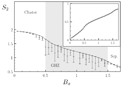
Figure 3: The bipartite reduced entropy $S_{2}$ for $J=0.5,B_{z}=0$ computed exactly through the Jordan-Wigner transform (full line) and through 40 runs of VMPS with 6 sweeps. Note that the cluster and separable phases compute the entanglement properties very precisely, especially away from the phase transitions, while in the Ising phase the results are much less reliable. Also, the algorithm inevitably underestimates the true value of $S_{2}$. The inset shows the local expectation value $\langle\sigma^{x}_{\mu}\rangle$, where error bars are too small to be evident. (N=200, D=8)

These results also show that $S_{2}$ is upper bounded by the true value, and the best representation can be chosen as those with the highest $S_{2}$ even when the exact value is not known.

IV.3 Numerical estimation of localizable entanglement

We now seek find an approximate MPS representation for the ground state of our model and with it, to compute the localizable entanglement. The latter step can be accomplished by a Monte-Carlo scheme Popp et al. (2005) to sample over entanglement by a weighted random walk in the probability space. Given that two substantial numerical steps are needed in this method to obtain the localizable entanglement, and in particular as a tendency of the MPS construction to occasionally yield incorrect representations of the ground state, the values obtained has an intrinsic error that we have indicated wherever applicable. Specifically, in the Ising phase, the method is unstable and picks out a ground state close to a product state rather than the GHZ state. However, we are interested in what happens in the cluster phase, and that problem is therefore not substantial. Importantly, the technique seems to be particularly well behaved in the cluster phase.

We use periodic boundary conditions (PBC) throughout, as this makes the computation much easier and, due to the resulting translation-invariance, reduces storage to only two matrices as opposed to $2N$ matrices in the open boundary condition case. As we show in Sec. VI, the $Z$ measurements do not perfectly disentangle the chain for $J>0$, and one might worry that the results are dependent on the boundary conditions as there are two directions in the lattice that the entanglement might propagate. However, our data show that this does not happen. Specifically, one can do $n_{z}$ subsequent $Z$ measurements, and for $n_{z}>1$, the resulting values for the entanglement is independent of $n_{z}$ for all $J$. Hence we are justified to use PBC, and the error in doing so is much smaller than the statistical noise of our methods, and we use $n_{z}=2$ in the following.

To estimate the localizable entanglement we must choose a specific measurement protocol, and the results of Sec. III reveal that the optimal basis for measuring the intermediate qubits is the $X$ basis. We measure the qubits beyond the endpoints in the $Z$ basis as for the cluster state.

Our numerics confirm our expectation that the localizable EL becomes finite for any $B_{z}>0$ (as can be shown analytically at $J=B_{x}=0$ using the MPS representation of Eq. 21). For the remainder of this paper, we restrict to $B_{z}=0$. We have computed the localizable entanglement along two lines in the phase diagram of Fig. 1: (i) $B_{x}=B_{z}=0$ and (ii) $B_{x}=.5$ and $B_{z}=0$. The (i) line will have an Ising class quantum phase transitions separating the cluster and Ising phases, while the (ii) line will have a phase transition at roughly $J=0.5$ between the same phases.

For the model with $\vec{B}=0$, the data clearly shows an infinite EL for $J<1$, and a significant localizable entanglement, as shown in Fig. 4. Similar results are found along the line (ii), with $B_{x}=0.5$.

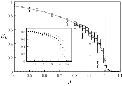
Figure 4: The localizable entanglement for a $N=60$ model with $\vec{B}=0$. MPSs used are $D=4$ (open circles) and $D=8$ (solid circles). The gray line is a guide to the eye, following the function $(1-J^{2})^{0.36}$, which is consistent with the expected behaviour of an second order phase transition order parameter. The error bars indicate the sensitivity of the initial conditions in the VMPS scheme. The inset shows a similar plot for $B_{x}=.5$ and $D=8$. Note that the performance of the VMPS is noticeably worse as $J$ approaches the phase transition, though the data are still conclusive.

The sensitivity on the initial conditions in the VMPS algorithm is far larger than the numerical errors of the Monte Carlo procedure. However, the latter is well suited to detect polynomial versus exponential decay, and performs consistently in this respect for different initial conditions even though the actual entanglement values may have substantial variation. Hence, we are able to separate an infinite EL phase (the cluster phase) and a finite EL phase.

V Characterizing entanglement in the cluster phase

We have shown both analytically and numerically that the localizable EL is diverging in the cluster phase, and the numerics also provide a mechanism to analyze the form of the resulting two-qubit entangled state. For $J>0$, the resulting two-qubit state is not identical to the form of the two-qubit cluster state even after the Pauli corrections. In this section, we explore the form of the post-measurement state and its dependence on the measurement results. We focus specifically on $\vec{B}=0$, but our results extend directly to $B_{x}>0$.

As we are performing the identical measurement sequence for localizing entanglement in the cluster state, it is natural to apply the same Pauli corrections to the final two-qubit state depending on the parity of the even and odd $X$-measurements, as well as the boundary $Z$-measurements. The correlation functions (16) which incorporate these corrections show that the resulting state does not take a fixed form. With the above Pauli corrections, the sampled states in the Monte Carlo analysis with near-maximal entanglement are characterized by $\langle\sigma^{y}_{a}\sigma^{y}_{b}\rangle_{\mathcal{P}}=1$, as expected from our analysis using the Jordan-Wigner transformation, as well as the relations

$$\langle\sigma^{z}_{a}\sigma^{x}_{b}\rangle_{\mathcal{P}}=\langle\sigma^{x}_{a}\sigma^{z}_{b}\rangle_{\mathcal{P}},\ \langle\sigma^{x}_{a}\sigma^{x}_{b}\rangle_{\mathcal{P}}=-\langle\sigma^{z}_{a}\sigma^{z}_{b}\rangle_{\mathcal{P}},$$ (25)

and

$$\langle\sigma^{z}_{a}\sigma^{x}_{b}\rangle_{\mathcal{P}}^{2}+\langle\sigma^{x}_{a}\sigma^{x}_{b}\rangle_{\mathcal{P}}^{2}=1\,.$$ (26)

(Sampled states that are not near-maximally entangled do not fall into this class.) The conditions (25) imply that the maximally entangled state are described by

$$|\Phi\rangle=\cos\Phi|C_{00}\rangle+\sin\Phi|C_{11}\rangle\,,$$ (27)

where we have defined

$$|C_{ij}\rangle=\left(\sigma^{x}_{b}\right)^{i}\left(\sigma^{z}_{b}\right)^{j}|C\rangle\qquad i,j=0,1\,.$$ (28)

This form of the states is consistent with the long-ranged behaviour of $\langle\sigma^{y}_{a}\sigma^{y}_{b}\rangle_{\mathcal{P}}$, but reveals an additional $y$-rotation by an angle $\Phi$.

Investigating the distribution of angles $\Phi$ for states sampled from the Monte Carlo analysis, we find that these angles do not take fixed multiples of $\pi/2$. This state may be corrected into the cluster state by a $y$-rotation of qubit $b$ by an angle $-\Phi$, but not by a Pauli correction. The angle $\Phi$ is a function of the measurement results, but we have been unable to determine this dependence.

We model $\Phi$ as sampled from a probability distribution $\mathcal{D}_{J}(\Phi)$, satisfying $\mathcal{D}_{0}(\Phi)=\delta(\Phi)$. We now show that this distribution does not possess any bias away from zero; if that were the case, one could improve the fidelity of the post-measurement state with the two-qubit cluster state by performing a correcting rotation. For a given $J$, the expectation value $\langle\sigma^{x}_{a}\sigma^{z}_{b}\rangle_{\mathcal{P}}$ will take the form

$$\langle\sigma^{x}_{a}\sigma^{z}_{b}\rangle_{\mathcal{P}}=A(J)\cos(\xi(J))\,,$$ (29)

where $A(0)=1$, $\xi(0)=0$. The phase $\xi(J)$ thereby determines the bias, and the amplitude $A$ gives the magnitude of the expectation value.

We can now investigate the behaviour of our localized entangled state as we approach the phase transition at $J=1$. We restrict our sampled states to maximally-entangled ones by projecting onto the subspace of states $|\Phi\rangle$, i.e. using a projector $P=|C_{00}\rangle\langle C_{00}|+|C_{11}\rangle\langle C_{11}|$. The probability of this projection viewed as a measurement is denoted $p_{yy}$; we note that this probability is large for all $J$ up to the phase transition as seen in the inset of Fig. 5.

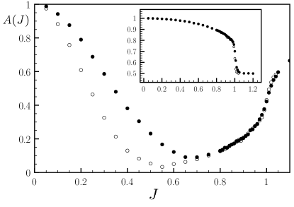
Figure 5: The amplitude $A(J)$ for the sinusoidal behavior of $\langle xz\rangle$ after a projection $P$ and $SO(2)$ correction on one qubit is done on the state. Closed circles are for $N=50$ while open circles are $N=102$. The inset shows the probability $p_{yy}$ of success for the measurement. Note that in the latter case the two system sizes are practically indistinguishable.

On states following the projection, we investigate the average angle. We find that the phase $\xi(J)$ is an indicator of a size-dependent transition, changing rapidly from zero to $\pi/2$, with a behavior closely approximated by

$$\xi(J)=\frac{\pi}{4}\left(\tanh\{K(N)[J-\eta(N)]\}+1\right)\,,$$ (30)

where the coefficients $K$ and $\eta$ are size dependent. The parameter $\eta$ is a good marker for the transition, and as shown in Fig. 6, it follows a power law $\eta\sim N^{-1/3}$, while $A$ increases non-universally with $N$. Up to this transition, there is no bias, and the state approximates a cluster state. Beyond this transition, the distribution $\mathcal{D}_{J}(\Phi)$ is almost uniform, meaning that there is no rotation independent of the measurement results that will increase the fidelity with the two-qubit cluster state.

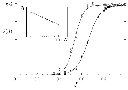
Figure 6: The phase $\xi(J)$ is shown for $N=50$ (closed circles) and $N=100$ (open circles). The error bars refer to the fitting to the sinusoidal curve. Full lines are best fits to $\tanh$, while the inset shows the scaling law for the transition parameter $\eta\sim N^{-1/3}$ on double log scale.

In summary, while the localizable EL remains infinite throughout the cluster phase, the resulting two-qubit entangled state cannot be deterministically transformed to the fiducial two-qubit cluster state using Pauli corrections for any $J>0$. Further work is required to determine the non-Pauli correction angle (about the $y$-axis) based on the measurement results. Potentially, this non-Pauli rotation could be useful for developing quantum computational wires Gross and Eisert (2008) that perform non-trivial single-qubit gates. However, without characterizing this rotation in terms of the measurement results, such states cannot be used directly as quantum computational wires.

VI Disentangling measurements

Finally, in addition to localizable entanglement, we consider another property of quantum states that is useful (though possibly not necessary) for measurement-based quantum computation. The cluster state possesses the useful property that a $Z$ measurement on any qubit “removes” that qubit and leaves the remaining qubits in a cluster state (up to a Pauli correction dependent on the measurement result). On a 1-D chain, a $Z$ measurement on a qubit will then disentangle the two halfs of the remaining chain. This property is shared by our model Hamiltonian for any $B_{z}$ as long as $B_{x}=J=0$ Barrett et al. (2008). If we turn instead to the model with $\vec{B}=0$ but $J>0$, we find that on an $N=3$ open chain, any measurement on the middle qubit will result in some remaining entanglement on the two end qubits, and therefore be an inadequate disentangling measurement.

In this section, we consider using local measurements on pairs of qubits that optimally disentangle the remaining halves of a 1-D chain with $\vec{B}=0$. (To be clear, we still consider single-qubit measurements, applied to two neighbouring qubits.) First, we consider both qubits to be measured at an angle $\vartheta$ in the $x{-}z$ plane. The outcomes $s$ are labelled according to the total spin in the desired direction which is either of $s=\{-1,0,1\}$. There are two outcomes with total spin zero, but these lead to identical states due to the reflection symmetry of the model and are therefore treated together. The optimal measurement angle depends on the measurement outcome, and this dependency is shown in Fig. 7.

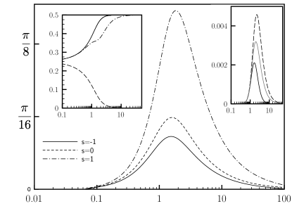
Figure 7: For a chain of 4 qubits, the measurement angle that disentangles the two extreme qubits is shown as a function of $J$ in the main panel. The left inset shows the corresponding outcome probabilities for the three possible measurement outcomes. The right inset shows the remaining entanglement multiplied with the probability of the outcome between the end qubits if no correction is done. In this case the outcomes $s=\pm 1$ are identical, so there are only two distinct cases, and the average entanglement is shown as a grey line.

Because the optimal measurement angle depends on the measurement outcome. Note that while all four measurement outcomes (there are two corresponding to $s=0$) are equally probable in the cluster state, the probability of the $s=0$ result vanishes for the GHZ state while the two remaining are equally probable.

Alternatively, one can view the measurement as a weak measurement described by four POVMs described in terms of the three measurement angles, $\vartheta_{p}$ with $p$ the measurement outcome, as shown in Fig. 7. The POVMs are thus

$$\begin{split}E_{-1}&=cM_{-}(\vartheta_{-1})\otimes M_{-}(\vartheta_{-1})\\ E_{0}&=cM_{-}(\vartheta_{0})\otimes M_{+}(\vartheta_{0})\\ E^{\prime}_{0}&=cM_{+}(\vartheta_{0})\otimes M_{-}(\vartheta_{0})\\ E_{1}&=cM_{+}(\vartheta_{1})\otimes M_{+}(\vartheta_{1})\\ E_{X}&=\mathds{1}-E_{-1}-E_{0}-E^{\prime}_{0}-E_{1},\end{split}$$ (31)

where $M_{\pm}(\vartheta)$ is a local projective measurement along the direction $\vartheta$, and the constant approximately $c\leq.5$ is required for $E_{X}$ to be positive in general. The element $E_{X}$, consisting of all local measurement outcomes that do not correspond to one of the others, is considered a ‘failure’ outcome. If this measurement result is obtained, the result must be discarded, while for any other result, the measurement sequence disentangles the two outer qubits. The probability of failure is $p(E_{X})=\langle\psi|E_{X}|\psi\rangle$. For the specific model in question, $c\leq.8$ is sufficient to retain positivity for all $J$. Since a higher $c$ means a lower probability of failure, on can further minimize failure by selecting the highest $c$ that allows for a positive $E_{X}$ for a specific set of measurement angles.

One may imagine that the POVM can be replaced by a projective two-qubit measurement, or equivalently that one can make adaptive measurements without postselection. However, this is not possible for any $0<J<\infty$. Consider making two measurements in the four qubit chain with different angles, $\theta_{1}$ and $\theta_{2}$. Mapping out the combinations that disentangle the chain for all four measurement outcomes, a pure projective measurement would be possible if all four lines crossed at some combination, while an adaptive or entangled measurement if one (say) $\theta_{1}$ for an outcome meant one could pick out a definite $\theta_{2}$ depending on the outcome and be ensured disentanglement. However, our numerical investigation has determined that this situation does not occur for any finite $J$. Hence, postselection is the only way to ensure disentanglement.

Note that these results for the $N=4$ chain cannot be immediately extrapolated to a general $N$ qubit chain, but the same general results hold, and a disentangling measurement can still be constructed by equal measurements on the $(N-2)/2$ middle qubit pairs with disentangling angles close to those described here.

VII Conclusions

For a 1D spin chain for which the ground state is a cluster state, we have demonstrated the existence of a robust “cluster phase” under local ($B_{x}$-field) and coupled (Ising) perturbations. All states in this phase exhibit diverging localizable EL. However, as we have been unable to determine the bi-product unitary as a function of the measurement results, the usefulness of such states as a quantum computational wire may be limited.

The existence of this cluster phase in one dimension may be extended to two dimensions even though our current numerical procedures are unlikely to be suitable for this. When extending to higher dimensions by similar schemes to MPS Bañuls et al. (2008), the entanglement properties are likely to be even harder to distill. Alternative techniques beyond the MPS paradigm may be more suitable Evenbly and Vidal (2009).

Appendix A Jordan-Wigner transform

The Jordan Wigner transform Jordan and Wigner (1928) is a mapping from the spins defined by the Pauli operators into spinless fermions, and is a standard technique in condensed matter physics. We give a quick overview here, and show how to obtain the relevant correlation functions. For a $N$ qubit chain, $N$ spinless fermions are defined by annihilation operators

$$a_{\mu}=\frac{1}{2}\left(\prod_{\nu<\mu}\sigma^{z}_{\nu}\right)(\sigma^{x}_{\mu}+i\sigma^{y}_{\mu})$$

and the adjoint creation operators. Futher one defines $2N$ self adjoint Majorana fermions

$$\gamma_{2\mu-1}=\frac{1}{i\sqrt{2}}\left(a_{\mu}-a^{\dagger}_{\mu}\right)\quad\gamma_{2\mu}=\frac{1}{\sqrt{2}}\left(a_{\mu}+a^{\dagger}_{\mu}\right)$$

where $\{\gamma_{i},\gamma_{j}\}=\delta_{ij}$. Switching coordinates $x\leftrightarrow z$ for the Hamiltonian (5) with $B_{z}=0$ gives

$$H=\sum_{ij}\gamma_{i}\mathcal{C}_{ij}\gamma_{j}$$

with the $2N\times 2N$ matrix

$$\mathcal{C}=i\begin{pmatrix}\mathcal{B}&\mathcal{J}&\mathcal{I}&0&\cdots&P\mathcal{I}^{\mathrm{T}}&P\mathcal{J}^{\mathrm{T}}\\ -\mathcal{J}^{\mathrm{T}}&\mathcal{B}&\mathcal{J}&\mathcal{I}&\cdots&0&P\mathcal{I}^{\mathrm{T}}\\ -\mathcal{I}^{\mathrm{T}}&-\mathcal{J}^{\mathrm{T}}&\mathcal{B}&\mathcal{J}&&\cdots&0\\ 0&-\mathcal{I}^{\mathrm{T}}&-\mathcal{J}^{\mathrm{T}}&\mathcal{B}&&\cdots&0\\ &&\vdots\\ -P\mathcal{J}&-P\mathcal{I}&0&\cdots&-\mathcal{I}^{\mathrm{T}}&-\mathcal{J}^{\mathrm{T}}&\mathcal{B}\end{pmatrix}$$

where

$$\mathcal{B}=\begin{pmatrix}0&-B_{x}\\ B_{x}&0\end{pmatrix}\quad\mathcal{J}=\begin{pmatrix}0&J\\ 0&0\end{pmatrix}\quad\mathcal{I}=\begin{pmatrix}0&1\\ 0&0\end{pmatrix}$$

and $P=\prod\sigma^{z}_{\mu}=\pm 1$ is the parity of the model which is a conserved quantity, $[H,P]=0$. If one considers a chain with open boundary conditions this simply amounts to setting $P=0$. It is not immediately obvious which parity segment the ground state belongs to, but this is easy to verify by computing the two energies. For large $N$ the difference between the two obtained states are in any respect very small.

Define the correlation matrix $\Gamma_{ij}=\langle[\gamma_{i},\gamma_{j}]\rangle$, in which every second entry is zero since $\langle\gamma_{2\mu}\gamma_{2\nu}\rangle=\langle\gamma_{2\mu+1}\gamma_{2\nu+1}\rangle=0$. This enables us to compute the von Neumann entropy of any subset of qubits effectively Latorre et al. (2004), and expectation values also follow easily.

The local $z$ expectation value (which corresponds to $x$ in the original coordinates) is simply $\langle\sigma^{z}_{\mu}\rangle=\Gamma_{2\mu-1,2\mu}=\Gamma_{12}$ where the last step is valid under PBC, or $P\not=0$. As an example of a more complicated expectation value, consider (16a), which in the current coordinates and transformed to Majorana fermions is

$$\mathcal{O} =\langle\sigma^{x}_{2}\sigma^{z}_{3}\sigma^{z}_{5}\cdots\sigma^{z}_{N-1}\sigma^{x}_{N}\rangle$$

$$=\langle\gamma_{3}\left(\prod_{k=1}^{N/2-2}\gamma_{4k+3}\gamma_{4(k+1)}\right)\gamma_{2N}\rangle.$$

Using Wick’s theorem, and the fact that only odd/even combinations of indices couples, one finds that $\mathcal{O}=\det G$ where $G$ is a submatrix of $\Gamma$,

$$G=\begin{pmatrix}\Gamma_{3,8}&\Gamma_{3,12}&\Gamma_{3,16}&\cdots&\Gamma_{3,2N-4}&\Gamma_{3,2N}\\ \Gamma_{7,8}&\Gamma_{7,12}&\Gamma_{7,16}&\cdots&\Gamma_{7,2N-4}&\Gamma_{7,2N}\\ \Gamma_{11,8}&&\cdots\\ \vdots\\ \Gamma_{2N-5,8}&\Gamma_{2N-5,12}&&\cdots&&\Gamma_{2N-5,2N}\end{pmatrix}.$$

Indeed, any expectation value is the determinant of a dense submatrix of $\Gamma$, the size of which depends on the expectation value in question.

References

- Briegel et al. (2009) H. J. Briegel, D. E. Browne, W. Dür, R. Raussendorf, and M. van den Nest, Nat. Phys. 5, 19 (2009).
- Nielsen and Chuang (2000) M. Nielsen and I. Chuang, Quantum Computation and Quantum Information (Cambridge University Press, 2000).
- Raussendorf et al. (2003) R. Raussendorf, D. E. Browne, and H. J. Briegel, Phys. Rev. A 68, 022312 (2003).
- Raussendorf et al. (2005) R. Raussendorf, S. Bravyi, and J. Harrington, Phys. Rev. A 71, 062313 (2005).
- Raussendorf et al. (2007) R. Raussendorf, J. Harrington, and K. Goyal, New J. Phys. 9, 199 (2007).
- Gross and Eisert (2007) D. Gross and J. Eisert, Phys. Rev. Lett. 98, 220503 (2007).
- Gross et al. (2007) D. Gross, J. Eisert, N. Schuch, and D. Perez-Garcia, Phys. Rev. A 76, 052315 (2007).
- van den Nest et al. (2007) M. van den Nest, W. Dur, A. Miyake, and H. J. Briegel, New J. Phys. 9, 204 (2007).
- Brennen and Miyake (2008) G. K. Brennen and A. Miyake, Phys. Rev. Lett. 101, 010502 (2008).
- Doherty and Bartlett (2008) A. C. Doherty and S. D. Bartlett, Phys. Rev. Lett. 103, 020506(2009).
- Barrett et al. (2008) S. D. Barrett, S. D. Bartlett, A. C. Doherty, D. Jennings, and T. Rudolph (2008), arXiv:0807.4797.
- Gross et al. (2009) D. Gross, S. T. Flammia, and J. Eisert, Phys. Rev. Lett. 102, 190501 (2009).
- Bremner et al. (2009) M. J. Bremner, C. Mora, and A. Winter, Phys. Rev. Lett. 102, 190502 (2009).
- Gottesman and Chuang (1999) D. Gottesman and I. Chuang, Nature 402, 390 (1999).
- Chung et al. (2009) T. Chung, S. D. Bartlett, and A. C. Doherty, Can. J. Phys. 87, 219 (2009).
- Bartlett and Rudolph (2006) S. D. Bartlett and T. Rudolph, Phys. Rev. A 74, 040302(R) (2006).
- Griffin and Bartlett (2008) T. Griffin and S. D. Bartlett, Phys. Rev. A 78, 062306 (2008).
- Gross and Eisert (2008) D. Gross and J. Eisert (2008), arXiv:0810.2542.
- Popp et al. (2005) M. Popp, F. Verstraete, M. A. Martin-Delgado, and J. I. Cirac, Phys. Rev. A 71, 042306 (2005).
- Pachos and Plenio (2004) J. K. Pachos and M. B. Plenio, Phys. Rev. Lett. 93, 056402 (2004).
- Pfeuty (1970) P. Pfeuty, Ann. Phys. 57, 79 (1970).
- Skrøvseth and Olaussen (2005) S. O. Skrøvseth and K. Olaussen, Phys. Rev. A 72, 022318 (2005).
- Verstraete et al. (2004a) F. Verstraete, M. Popp, and J. I. Cirac, Phys. Rev. Lett. 92, 027901 (2004a).
- Venuti and Roncaglia (2005) L. C. Venuti and M. Roncaglia, Phys. Rev. Lett. 94, 207207 (2005).
- Tagliacozzo et al. (2008) L. Tagliacozzo, T. R. de Oliveira, S. Iblisdir, and J. I. Latorre, Phys. Rev. B 78, 024410 (2008).
- Wolf et al. (2006) M. M. Wolf, G. Ortiz, F. Verstraete, and J. I. Cirac, Phys. Rev. Lett. 97, 110403 (2006).
- White (1992) S. R. White, Phys. Rev. Lett. 69, 2863 (1992).
- Pérez-García et al. (2007) D. Pérez-García, F. Verstraete, M. Wolf, and J. Cirac, Quantum Inf. Comput. 7, 401 (2007).
- Verstraete et al. (2004b) F. Verstraete, M. Martin-Delgado, and J. I. Cirac, Phys. Rev. Lett. 92, 087201 (2004b).
- Schuch et al. (2008) N. Schuch, I. Cirac, and F. Verstraete, Phys. Rev. Lett. 100, 250501 (2008).
- Verstraete et al. (2004c) F. Verstraete, D. Porras, and J. I. Cirac, Phys. Rev. Lett. 93, 227205 (2004c).
- Bañuls et al. (2008) M. Bañuls, D. Pérez-García, M. Wolf, F. Verstraete, and J. I. Cirac, Phys. Rev. A 77, 052306 (2008).
- Evenbly and Vidal (2009) G. Evenbly and G. Vidal, Phys. Rev. B 79, 144108 (2009).
- Jordan and Wigner (1928) P. Jordan and E. Wigner, Z. Physik 47, 631 (1928).
- Latorre et al. (2004) J. Latorre, E. Rico, and G. Vidal, Quant. Inf. Comput. 4, 48 (2004).