Analytic description of atomic interaction at ultracold temperatures: the case of a single channel

Abstract

We present analytic descriptions of atomic interaction at ultracold temperatures using both single-channel and multichannel quantum-defect theories. In the case of a single channel, addressed in this paper, the expansion of [B. Gao, Phys. Rev. A 58, 4222 (1998)] is generalized to higher orders for angular momentum $l\geq 2$ to give a more complete description of ultracold scattering, including an analytic description of ultracold shape resonances of arbitrary $l$. We also introduce a generalized scattering length that is well defined and useful for all partial waves, to replace the traditional definition that fails for $l\geq 2$ due to the long-range van der Waals interaction. The results are used in a companion paper to derive analytic descriptions of atomic interaction around a magnetic Feshbach resonance of arbitrary angular momentum $l$.

I Introduction

One of the key factors that has made cold-atom physics such a thriving field has been the tunability of atomic interaction via Feshbach, especially magnetic Feshbach resonances Tiesinga et al. (1993); Köhler et al. (2006); Chin et al. (2008). While the $s$ wave Feshbach resonances have received most of the attention for many years, the same concept is of course equally applicable to any other, nonzero partial waves. A number of such resonances have been observed experimentally Regal et al. (2003); Ticknor et al. (2004); Zhang et al. (2004); Schunck et al. (2005); Gaebler et al. (2007); Chin et al. (2008), including a recent observation of a Feshbach resonance of $l=8$ Knoop et al. (2008). Before we can understand questions such as what happens to a few-atom or a many-atom quantum system when a $p$ wave or a $d$ wave Feshbach resonance is tuned around the threshold, we need first to understand the corresponding two-atom system, namely, how to describe atom-atom scattering and atom-atom bound state with a Feshbach resonance of angular momentum $l$ around the threshold. This is the subject of this and a companion study.

Recall that for the $s$ wave, a magnetic Feshbach resonance can be conveniently described by Moerdijk et al. (1995)

$$a_{l=0}(B)=a_{bgl=0}\left(1-\frac{\Delta_{Bl=0}}{B-B_{0l=0}}\right)\;.$$ (1)

Here $a_{l=0}$ represents the $s$ wave scattering length, which is tunable by the magnetic field, $B$, around a Feshbach resonance, $a_{bgl=0}$ is a background scattering length, $\Delta_{Bl=0}$ is a measure of the width of the resonance, and $B_{0l=0}$ is the magnetic field at which $a_{l=0}=\infty$, corresponding to having a quasibound $s$ state right at the threshold. Once the scattering length is determined, the scattering properties above the threshold, or the binding energy of an atom pair with large and positive scattering lengths, can be determined, at least to a degree Köhler et al. (2006); Chin et al. (2008), from the effective-range theory (ERT) Schwinger (1947); Blatt and Jackson (1949); Bethe (1949), which, for positive energies, corresponds to the expansion

$$k^{2l+1}\cot\delta_{l}=-\frac{1}{{a}_{l}}+\frac{1}{2}{r}_{el}k^{2}+\cdots\;,$$ (2)

where $r_{el}$ is called the effective range.

The situation for $l\neq 0$ is considerably more complex due to the long-range van der Waals interaction, $-C_{6}/r^{6}$, between atoms. First, we have the obvious problem that the scattering length is not defined for $l\geq 2$ Levy and Keller (1963); Gao (1998a), meaning that the energy dependence of the scattering phase shift will necessarily differ from that implied by Eq. (2). Second, a Feshbach resonance of $l\neq 0$, when slightly above the threshold, is in fact a Feshbach/shape resonance, the atoms in such a state see the angular-momentum barrier just like they would in a single channel shape resonance state. When such a Feshbach resonance is tuned from above to below the threshold, its width, due to the presence of the angular momentum barrier, can be expected to become increasingly narrow and approaches zero when it crosses the threshold to become a true bound state. Any complete theory for a Feshbach resonance of $l\neq 0$ has to be able to describe this increasingly rapid energy variation as it approaches the threshold.

It is thus not surprising that the key to understanding Feshbach resonances of $l\neq 0$, to be presented in a companion paper, turns out to be the understanding of single channel shape resonances at ultracold energies, or equivalently, the threshold behaviors of single channel shape resonances, which is addressed in detail in this work. We point out that this is a nontrivial problem that, to the best of our knowledge, has not been done except for the $p$ wave description in Ref. Gao (1998a). Part of the difficulty can be attributed to the breakdown of the semiclassical approximation around the threshold Williams (1945); Kirschner and Le Roy (1978); Julienne and Mies (1989); Gribakin and Flambaum (1993); Trost et al. (1998a); Boisseau et al. (1998); Trost et al. (1998b); Flambaum et al. (1999); Gao (1999, 2008), which implies, in particular, that the tunneling amplitude or probability through the angular momentum barrier Gao (2008) cannot be obtained semiclassically.

Our analytic description of ultracold shape resonances is based on the small energy expansion of the quantum-defect theory (QDT) for $-1/r^{6}$ type of interactions Gao (1998a, 2001, 2008). It is presented here in a general analytic framework for ultracold atomic interaction that we call the QDT expansion, which is applicable with or without the presence of ultracold shape resonances. The presentation is organized as follows. In Sec. II, we generalize the single-channel QDT expansion of Ref. Gao (1998a) to higher orders for $l\geq 2$ to give us a more complete description of atom-atom scattering around the threshold, including an analytic description of the threshold behaviors of single-channel shape resonances. In Sec. III, we present further understanding of ultracold shape resonances by extracting from the QDT expansion analytic formulas for their position, width, and background. In Sec. IV, we derive from the QDT expansion a generalized effective-range expansion, from which we introduce the concepts of a generalized scattering length and a generalized effective range that are well defined for all angular momenta $l$. In Sec. V, we summarize the QDT expansions, derived previously in Ref. Gao (2004a), for the binding energies of the least-bound molecular state of arbitrary angular momentum $l$, using the standardized notations of Ref. Gao (2008) that we adopt here. We also present in this section a few intermediate results that will be useful in studying magnetic Feshbach resonances of arbitrary $l$. Further comments and remarks on the theory are presented in Sec. VI, with conclusions given in Sec. VII. The appendix presents analytic results of generalized scattering lengths and other QDT parameters, for arbitrary $l$, for two types of model potentials, a hard sphere with an attract tail of the type of $-C_{6}/r^{6}$, and the Lennard-Jones potential of the type of LJ(6,10).

The analytic description of atomic interaction around a magnetic Feshbach resonance of arbitrary $l$, which is necessarily multichannel in nature Tiesinga et al. (1993); Köhler et al. (2006); Chin et al. (2008), is developed in a companion paper. It will be accomplished through first, a rigorous reduction of the underlying multichannel problem, as described by the multichannel quantum-defect theory (MQDT) for $-1/r^{6}$ type of interactions Gao et al. (2005), to an effective single-channel problem, and a subsequent application of the results of this work.

II QDT expansion for single-channel scattering

In this section, we derive and discuss the QDT expansion for single-channel scattering. It differs considerably from the ERT Schwinger (1947); Blatt and Jackson (1949); Bethe (1949), which assumes that $k^{2l+1}\cot\delta_{l}$ is both an analytic and a slowly varying function of energy around the threshold, and can therefore can be approximated by the first few terms in its energy expansion. The QDT expansion makes no such assumptions. The only quantities expanded are the universal functions of a scaled energy that are associated with the long-range potential Gao (2008). There is no assumption about how $k^{2l+1}\cot\delta_{l}$ or $\tan\delta_{l}$ may vary with energy. It is partly for this reason that the QDT expansion can give analytic description of an ultracold shape resonance, which has rapid energy dependence that would have required, at least, partial summation over all orders of energy in more standard approaches. The QDT expansion is also more than a small-energy expansion. It is simultaneously a large-$l$ expansion, in the sense that for any fixed energy, there is a sufficiently large $l$ beyond which it becomes applicable. As a related consequence, the energy range over which the QDT expansion is applicable increases rapidly for larger $l$.

While the derivation of the QDT expansion is somewhat tedious, the end result will be very simple. It is given by a single analytic formula applicable to all angular momentum $l$ and regardless of whether there is, or is not, an ultracold shape resonance. To make the derivation easier to follow, we first rewrite, in Sec. II.1, the QDT for single channel scattering Gao (1998a, 2001, 2008) in a form that makes its subsequent expansion, presented and discussed in Sec. II.2, fully transparent.

II.1 QDT for single-channel scattering

For a single channel problem with long-range $-C_{6}/r^{6}$ interaction, the scattering above the threshold is described rigorously in the QDT by the following equation for the $K$ matrix Gao (1998a, 2001, 2008)

$$K_{l}=\tan\delta_{l}=(Z^{c}_{gc}K^{c}-Z^{c}_{fc})(Z^{c}_{fs}-Z^{c}_{gs}K^{c})^{-1}\;.$$ (3)

Here $K^{c}(\epsilon,l)$ is a short-range $K$ matrix that depends weakly on both the energy $\epsilon$ and the angular momentum $l$ Gao (2008). The $Z^{c}_{xy}$ are elements of the $Z^{c}$ matrix for the $-1/r^{6}$ type of potentials, labeled here using the standardized notation of Ref. Gao (2008). They are given explicitly by

$$Z^{c}_{fs} = A^{Z}_{l}\left\{\left[1-(-1)^{l}M_{\epsilon_{s}l}\tan\pi(\nu-\nu_{0})\right]\sin(\pi\nu/2)X_{l}\right.$$ (4)

$$+\left.\left[1+(-1)^{l}M_{\epsilon_{s}l}\tan\pi(\nu-\nu_{0})\right]\cos(\pi\nu/2)Y_{l}\right\},$$

$$Z^{c}_{fc} = A^{Z}_{l}\left\{\left[\tan\pi(\nu-\nu_{0})-(-1)^{l}M_{\epsilon_{s}l}\right]\sin(\pi\nu/2)X_{l}\right.$$ (5)

$$+\left.\left[\tan\pi(\nu-\nu_{0})+(-1)^{l}M_{\epsilon_{s}l}\right]\cos(\pi\nu/2)Y_{l}\right\},$$

$$Z^{c}_{gs} = A^{Z}_{l}\left\{\left[1+(-1)^{l}M_{\epsilon_{s}l}\tan\pi(\nu-\nu_{0})\right]\cos(\pi\nu/2)X_{l}\right.$$ (6)

$$-\left.\left[1-(-1)^{l}M_{\epsilon_{s}l}\tan\pi(\nu-\nu_{0})\right]\sin(\pi\nu/2)Y_{l}\right\},$$

$$Z^{c}_{gc} = A^{Z}_{l}\left\{\left[\tan\pi(\nu-\nu_{0})+(-1)^{l}M_{\epsilon_{s}l}\right]\cos(\pi\nu/2)X_{l}\right.$$ (7)

$$-\left.\left[\tan\pi(\nu-\nu_{0})-(-1)^{l}M_{\epsilon_{s}l}\right]\sin(\pi\nu/2)Y_{l}\right\},$$

where

$$A^{Z}_{l}=\frac{G_{\epsilon_{s}l}(\nu)\cos\pi(\nu-\nu_{0})}{\sqrt{2}(X_{l}^{2}+Y_{l}^{2})\sin\pi\nu}\;,$$

$\nu_{0}=(2l+1)/4$, $M_{\epsilon_{s}l}=G_{\epsilon_{s}l}(-\nu)/G_{\epsilon_{s}l}(\nu)$, with the characteristic exponent $\nu$, and functions $X_{l}$, $Y_{l}$, and $G_{\epsilon_{s}l}$ being defined in Ref. Gao (1998b). They are all universal functions of a scaled energy,

$$\epsilon_{s}=\epsilon/s_{E}\;,$$ (8)

where $s_{E}=(\hbar^{2}/2\mu)(1/\beta_{6})^{2}$ is the energy scale corresponding to the length scale $\beta_{6}=(2\mu C_{6}/\hbar^{2})^{1/4}$ that is associated with the $-C_{6}/r^{6}$ potential. For the purpose of providing orders of magnitudes, these scales, and also the related time scale, $s_{T}=\hbar/s_{E}$, are tabulated in Table 1 for selected alkali-metal dimers. They are all determined by the $C_{6}$ coefficient and the reduced mass $\mu$.

Table 1: Sample scale parameters for $A+A$ type of systems where $A$ is an alkali-metal atom. The $\beta_{6}=(2\mu C_{6}/\hbar^{2})^{1/4}$ is the length scale. The $s_{E}=(\hbar^{2}/2\mu)(1/\beta_{6})^{2}$ is the corresponding energy scale. It is given both in units of $\mu$K and in units of MHz. $s_{T}=\hbar/s_{E}$ is the corresponding time scale. All are determined by the $C_{6}$ coefficient and atomic masses.

Atom	$C_{6}$ (a.u.)	$\beta_{6}$ (a.u.)	$s_{E}/k_{B}$ ($\mu$K)	$s_{E}/h$ (MHz)	$s_{T}$ (ns)
6Li	1393.39	$62.52$	$7368$	$153.5$	$1.037$
23Na	$1556$	$89.86$	$933.1$	$19.44$	$8.186$
40K	3897	$129.8$	$257.3$	$5.360$	$29.69$
85Rb	$4707$	$164.3$	$75.58$	$1.575$	$101.1$
133Cs	6860	$201.9$	$31.97$	$0.6662$	$238.9$

Equation (3) gives an exact description of single-channel atomic scattering in terms of a set of universal functions determined solely by the long-range interaction. All the short-range physics are encapsulated in $K^{c}(\epsilon,l)$, which is slowly varying in both $\epsilon$ and $l$ around the threshold Gao (2008).

Instead of the $K^{c}$ parameter, the short-range atomic interaction in any partial wave can also be described using alternative parameters such as the quantum-defect $\mu^{c}$ or the parameter $K^{c0}_{l}$ Gao (2008). They are all related, but have different utilities for different purposes. For this work, which focuses on the ultracold regime around the threshold, the most convenient parameter is $K^{c0}_{l}$. It is defined as the short-range $K$ matrix associated with the $f^{c0}$ and $g^{c0}$ reference pair of Ref. Gao (2008), and is related, for $-1/r^{6}$ type of potentials, to the $K^{c}$ and $\mu^{c}$ by

$$K^{c0}_{l}(\epsilon) = \frac{K^{c}(\epsilon,l)-\tan(\pi\nu_{0}/2)}{1+\tan(\pi\nu_{0}/2)K^{c}(\epsilon,l)}\;,$$ (9)

$$= \tan[\pi\mu^{c}(\epsilon,l)-l\pi/4]\;.$$ (10)

With this definition, $K^{c0}_{l}(\epsilon=0)=0$ corresponds to having a bound or quasibound state of angular momentum $l$ right at the threshold, a small and positive $K^{c0}_{l}(0)$ corresponds to having a bound state of $l$ close to the threshold, and a small and negative $K^{c0}_{l}(0)$ corresponds to having a shape resonance of angular momentum $l$ close to the threshold Gao (2000, 2004b, 2004a). This property of $K^{c0}_{l}$, which was called $x_{l}$ in Refs. Gao (2004b, a) and is related to the $K^{0}_{l}$ of Ref. Gao (1998a) by $K^{c0}_{l}=-K^{0}_{l}$, allows it to be used as an expansion parameter when there is a state close to the threshold Gao (2004a). As will become clear later in the paper, $K^{c0}_{l}$ is also the short-range parameter that has the simplest relation to the scattering lengths and the generalized scattering lengths.

Defining $\theta_{l}$ by

$$\sin\theta_{l} = Y_{l}(X_{l}^{2}+Y_{l}^{2})^{-1/2}\;,$$ (11)

$$\cos\theta_{l} = X_{l}(X_{l}^{2}+Y_{l}^{2})^{-1/2}\;,$$ (12)

the elements of the $Z^{c}$ matrix can be further written as

$$Z^{c}_{fs} = B^{Z}_{l}\left[\sin\left(\frac{1}{2}\pi\nu+\theta_{l}\right)\right.$$ (13)

$$\left.-(-1)^{l}M_{\epsilon_{s}l}\tan\pi(\nu-\nu_{0})\sin\left(\frac{1}{2}\pi\nu-\theta_{l}\right)\right]\;,$$

$$Z^{c}_{fc} = B^{Z}_{l}\left[\tan\pi(\nu-\nu_{0})\sin\left(\frac{1}{2}\pi\nu+\theta_{l}\right)\right.$$ (14)

$$\left.-(-1)^{l}M_{\epsilon_{s}l}\sin\left(\frac{1}{2}\pi\nu-\theta_{l}\right)\right]\;,$$

$$Z^{c}_{gs} = B^{Z}_{l}\left[\cos\left(\frac{1}{2}\pi\nu+\theta_{l}\right)\right.$$ (15)

$$\left.+(-1)^{l}M_{\epsilon_{s}l}\tan\pi(\nu-\nu_{0})\cos\left(\frac{1}{2}\pi\nu-\theta_{l}\right)\right]\;,$$

$$Z^{c}_{gc} = B^{Z}_{l}\left[\tan\pi(\nu-\nu_{0})\cos\left(\frac{1}{2}\pi\nu+\theta_{l}\right)\right.$$ (16)

$$\left.+(-1)^{l}M_{\epsilon_{s}l}\cos\left(\frac{1}{2}\pi\nu-\theta_{l}\right)\right]\;,$$

where

$$B^{Z}_{l}=\frac{G_{\epsilon_{s}l}(\nu)\cos\pi(\nu-\nu_{0})}{\sqrt{2}(X_{l}^{2}+Y_{l}^{2})^{1/2}\sin\pi\nu}\;.$$ (17)

Substituting Eqs. (13)-(16) into Eq. (3) and using $K^{c0}_{l}(\epsilon)$ as the short-range parameter, we can rewrite the QDT equation for the $K$ matrix as

$$K_{l}=\tan\delta_{l}=-\tan[\pi(\nu-\nu_{0})]-\widetilde{A}_{ls}(\epsilon_{s})k_{s}^{2l+1}\frac{1-\tan^{2}[\pi(\nu-\nu_{0})]}{1+\widetilde{A}_{ls}(\epsilon_{s})k_{s}^{2l+1}\tan[\pi(\nu-\nu_{0})]}\;,$$ (18)

where $k_{s}=\epsilon_{s}^{1/2}=k\beta_{6}$, and

$$\widetilde{A}_{ls}(\epsilon_{s})=\left[\frac{(-1)^{l}M_{l}\sin\pi\nu_{0}}{k_{s}^{2l+1}}\right]\frac{[1+(-1)^{l}K^{c0}_{l}]\{1+\tan\theta_{l}\tan[\pi(\nu-\nu_{0})/2]-[(-1)^{l}-K^{c0}_{l}]\{\tan\theta_{l}-\tan[\pi(\nu-\nu_{0})/2]\}}{K^{c0}_{l}-\tan\theta_{l}-\tan[\pi(\nu-\nu_{0})/2]-K^{c0}_{l}\tan\theta_{l}\tan[\pi(\nu-\nu_{0})/2]}\;.$$ (19)

This is still an exact expression for $K_{l}$, and it has been written in a way to make its QDT expansion fully transparent.

II.2 QDT expansion

For small energies around the threshold, or for arbitrary energy but sufficiently large $l$, the quantities in Eq. (18) can be represented by expansions Gao (2004a) that derive straightforwardly from the analytic solution for the $-1/r^{6}$ type of potential Gao (1998b):

$$\nu-\nu_{0}=-\frac{3}{2^{5}\nu_{2}(\nu_{2}^{2}-1)(\nu_{2}^{2}-4)}\epsilon_{s}^{2}+O(\epsilon_{s}^{4})\;,$$ (20)

$$\tan\theta_{l}=-\frac{1}{2^{2}(\nu_{2}^{2}-1)}\epsilon_{s}+O(\epsilon_{s}^{3})\;,$$ (21)

$$M_{\epsilon_{s}l} = (-1)^{l}\frac{\pi^{2}}{2^{4\nu_{2}-1}\sin(\pi\nu_{0})}\frac{1}{[\Gamma(\nu_{0})\Gamma(\nu_{2}+1)]^{2}}|\epsilon_{s}|^{\nu_{2}}$$ (22)

$$\times\left\{1+2(\nu-\nu_{0})\ln|\epsilon_{s}|-\left[(-1)^{l}\pi+8\ln 2+\frac{4}{\nu_{2}}+2\psi(\nu_{0})\right](\nu-\nu_{0})\right.$$

$$\left.+\frac{1}{2^{6}\nu_{2}}\left[\frac{1}{(\nu_{2}+1)^{2}(\nu_{2}+2)}-\frac{16}{(\nu_{2}^{2}-4)^{2}}-\frac{1}{(\nu_{2}-1)^{2}(\nu_{2}-2)}\right]\epsilon_{s}^{2}\right\}$$

$$+O\left[|\epsilon_{s}|^{\nu_{2}+4}(\ln|\epsilon_{s}|)^{2}\right]\;,$$

where $\nu_{0}=(2l+1)/4$, as defined earlier, $\nu_{2}\equiv 2\nu_{0}=l+1/2$, and $\psi(x)$ is the digamma function Abramowitz and Stegun (1964).

Combining these expansions with Eqs. (18) and (19) shows that the $K$ matrix has the following structure

$$\tan\delta_{l}=-\pi(\nu-\nu_{0})-\bar{a}_{sl}k_{s}^{2l+1}\frac{1+(-1)^{l}K^{c0}_{l}-[(-1)^{l}-K^{c0}_{l}][\theta_{l}-\pi(\nu-\nu_{0})/2]+O(k_{s}^{6})}{K^{c0}_{l}-\theta_{l}-\pi(\nu-\nu_{0})/2+O(k_{s}^{6})}\left[1+O(k_{s}^{4}\ln k_{s})\right]+O(k_{s}^{8})\;,$$ (23)

where

$$\bar{a}_{sl} = \frac{\pi^{2}}{2^{4l+1}[\Gamma(l/2+1/4)\Gamma(l+3/2)]^{2}}$$ (24)

$$= \frac{\pi}{2^{2l-1}[\Gamma(l/2+1/4)]^{2}[(2l+1)!!]^{2}}\;,$$

is what we call the scaled mean scattering length for angular momentum $l$. It is a generalization of the $s$ wave mean scattering length of Gribakin and Flambaum Gribakin and Flambaum (1993) to $p$ Gao (2004a) and higher partial waves. More explicitly,

$$\bar{a}_{sl=0}=\frac{2\pi}{[\Gamma(1/4)]^{2}}\approx 0.4779888\;,$$ (25)

$$\bar{a}_{sl=1}=\frac{[\Gamma(1/4)]^{2}}{36\pi}\approx 0.1162277\;.$$ (26)

For larger $l$, it decreases rapidly and can be either computed directly or obtained from $\bar{a}_{sl=0}$ and $\bar{a}_{sl=1}$ using the recurrence relation

$$\bar{a}_{sl+2}=\frac{1}{[(2l+5)(2l+3)(2l+1)]^{2}}\bar{a}_{sl}\;,$$ (27)

which gives, e.g., $\bar{a}_{sl=2}=\bar{a}_{sl=0}/225$. Together, they represent a set of universal numbers determined solely by the long-range potential. The corresponding mean scattering length, with scale included, is defined as $\bar{a}_{l}=\bar{a}_{sl}\beta_{6}^{2l+1}$.

Equation (23), if kept to the order of $k_{s}^{5}$, gives the following result for the $s$ wave

$$\tan\delta_{l=0}\approx\frac{\pi}{15}k_{s}^{4}-\bar{a}_{sl=0}k_{s}\frac{1+K^{c0}_{l}-(1-K^{c0}_{l})\left(\frac{1}{3}k_{s}^{2}+\frac{\pi}{30}k_{s}^{4}\right)}{K^{c0}_{l}-\frac{1}{3}k_{s}^{2}+\frac{\pi}{30}k_{s}^{4}}\left[1-\frac{4}{15}k_{s}^{4}\ln k_{s}+\frac{2}{15}\left(\frac{22}{5}+\ln 2-\gamma\right)k_{s}^{4}\right]\;,$$ (28)

where $\gamma=0.5772156649\dots$ is the Euler’s constant Abramowitz and Stegun (1964). Results of even higher orders are possible. An $s$ wave result to the order of $k_{s}^{6}$ was given in Ref. Gao (1998a). Similar results can be written down for other partial waves.

For the range of energies of interest in cold-atom physics, this level of complexity is actually unnecessary, especially for higher partial waves. For simplicity and easier application, we will use the following approximation of Eq. (23) for all $l$

$$\tan\delta_{l}\approx K^{(B)}_{l}+K^{(D)}_{l}\;,$$ (29)

where

$$K^{(B)}_{l} \approx -\pi(\nu-\nu_{0})$$ (30)

$$\approx \frac{3\pi}{(2l+5)(2l+3)(2l+1)(2l-1)(2l-3)}\epsilon_{s}^{2}\;,$$

is a term that could have been derived from the Born approximation (see, e.g., Ref. Landau and Lifshitz (1977)), and

$$K^{(D)}_{l}\approx-\widetilde{A}_{sl}(\epsilon_{s})k_{s}^{2l+1}\;,$$ (31)

describes the deviation from the Born term. Here

$$\widetilde{A}_{sl}(\epsilon_{s}) \approx \bar{a}_{sl}\left[(-1)^{l}+\frac{1+K^{c0}_{l}\theta_{l}}{K^{c0}_{l}-\theta_{l}-\pi(\nu-\nu_{0})/2}\right]\;,$$ (32)

$$= \bar{a}_{sl}\left[(-1)^{l}+\frac{(2l+3)(2l-1)-K^{c0}_{l}\epsilon_{s}}{(2l+3)(2l-1)K^{c0}_{l}+\epsilon_{s}+w_{l}\epsilon_{s}^{2}}\right]\;,$$ (33)

can be regarded as a scaled, energy-dependent, generalized scattering length. Both expressions for $\widetilde{A}_{sl}(\epsilon_{s})$ are useful for different purposes. In Eq. (33), $w_{l}$ is an $l$-dependent constant defined by

$$w_{l}=\frac{3\pi}{2(2l+5)(2l+1)(2l-3)}\;.$$ (34)

Equation (32), while less explicit compared to Eq. (33), is more convenient for a number of conceptual purposes. Here $\pi(\nu-\nu_{0})$ is given by Eq. (30), and $\theta_{l}$ is given by Eq. (21), or more explicitly by

$$\theta_{l}\approx-\frac{1}{(2l+3)(2l-1)}\epsilon_{s}\;.$$ (35)

Table 2: Critical scaled energies, $\epsilon_{scl}$, for different angular momentum $l$. Beyond $\epsilon_{scl}$, the characteristic exponent $\nu$ for the $-1/r^{6}$ solutions Gao (1998b) moves off the real axis and becomes complex.

$l$	$\epsilon_{scl}$	$l$	$\epsilon_{scl}$
0	$1.544707$	6	$94.82401$
1	$2.358067$	7	$212.3067$
2	$6.891073$	8	$206.8228$
3	$25.29322$	9	$406.8301$
4	$33.17273$	10	$383.5433$
5	$89.85261$	11	$687.4041$

Together, Eqs. (29)-(33) give a single analytic formula for low-energy atomic scattering that we call the QDT expansion. It is applicable to all $l$, with or without the presence of ultracold shape resonances. It has the following additional characteristics. (a) The QDT expansion remains applicable no matter how rapidly the $K^{c0}_{l}(\epsilon)$ parameter may depend on energy. In arriving at Eqs. (29)-(33), the only quantities that are expanded are the universal functions associated with the long-range potential. There is no assumption about the values of $K^{c0}_{l}(\epsilon)$, or how it may depend on energy. While this feature of the QDT expansion is not important for true single channel cases, for which the energy dependence of $K^{c0}_{l}$ is almost always negligible Gao (1998a, 2001), it will become crucial when we apply it to effective single channel problems that are derived from intrinsically multichannel ones, for which the energy dependence of $K^{c0}_{l}$ is generally important. (b) The energy range over which the QDT expansion is applicable increase rapidly with $l$, roughly as $l^{3}$. This is consistent with the fact that the QDT expansion is simultaneously a large $l$ expansion Gao (2004a). For any energy, there is a sufficiently large $l$ beyond which it becomes applicable. The only condition for the applicability of the QDT expansion is $\epsilon_{s}\ll\epsilon_{scl}$, where $\epsilon_{scl}$ is the scaled critical energy beyond which the characteristic exponent $\nu$ becomes complex Gao (1998b). Values of $\epsilon_{scl}$ for the first twelve partial waves are listed in Table 2. For large $l$, they correspond roughly to the scaled height of the angular momentum barrier, given for $-1/r^{6}$ type of potentials by $H_{sl}=(2/3^{3/2})[l(l+1)]^{3/2}$. As will be discussed in more detail elsewhere, the critical energy is also the energy around which the behavior of the system goes from being quantum to being semiclassical Flambaum et al. (1999); Gao (2008). Thus the QDT expansion can also be regarded as a quantum expansion, applicable over a quantum region of energies where the quantum reflection probability is close to 1 Gao (1998b).

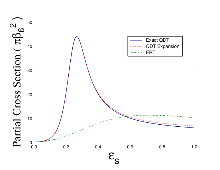
Figure 1: (Color online) $p$ wave partial cross sections for $a_{l=1}/\bar{a}_{l=1}=-20$ (corresponding to $K^{c0}_{l=1}\approx-0.0526$). Results of the QDT expansion (dashed line) are compared to the exact QDT results computed from Eq. (3) (solid line), and the results of ERT (dash-dot line).

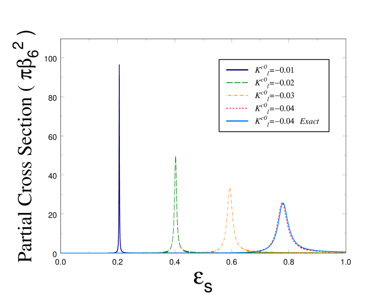
Figure 2: (Color online) $d$ wave shape resonances as described by the QDT expansion for different values of $K^{c0}_{l=2}$. The exact QDT results computed from Eq. (3) are only shown for $K^{c0}_{l=2}=-0.04$ as they become indistinguishable from those of QDT expansion for smaller $|K^{c0}_{l=2}|$. For higher partial waves, the QDT expansions are more accurate, and applicable over a greater range of scaled energies than shown here for the $d$ wave.

Figures 1 and 2 illustrate the QDT expansion for $p$ and $d$ waves, respectively, using cases that have a shape resonance in the threshold region. Since our interest here is in the case of a single channel, $K^{c0}_{l}$ is taken to be a constant Gao (1998a, 2001), $K^{c0}_{l}=K^{c0}_{l}(\epsilon=0)$, which is related in a simple way to the scattering length by Eq. (48) or (52), to be discussed in more details later. Note that the QDT expansion is applicable regardless of how narrow the shape resonances may be. In fact it is more accurate for narrower resonances which are necessarily located at smaller energies, as illustrated in Fig. 2. For higher partial waves, the results of the QDT expansion are no longer distinguishable from the exact QDT results, computed using Eq. (3), in the range of energies shown in Figs. 1 and 2. Such results are easily calculated from the analytic formula, and are therefore not shown.

Figure 1 is also used to illustrate the limitation of the ERT Schwinger (1947); Blatt and Jackson (1949); Bethe (1949). In the figure, the ERT results are computed from [see Eq. (2)]

$$k^{3}\cot\delta_{l=1}=-1/a_{l=1}\;.$$ (36)

Note that since the effective range is not defined for the $p$ wave due to the van der Waals interaction Levy and Keller (1963); Gao (1998a), it is incorrect to add an effective range term to Eq. (36). The lowest order correction to the right-hand-side of Eq. (36) is of the order $k$ (see Eqs. (29)–(33), or Ref. Gao (1998a)), not of the order of $k^{2}$ as implied by ERT. Figure 1 clear illustrates the failure of ERT, which misses the $p$ wave shape resonance completely. The consequence of such a failure for two atoms in a trap has been illustrated elsewhere Chen and Gao (2007). Careful readers should note that ERT description of $p$ wave interaction is still sometimes incorrectly used in the literature. This is unfortunate, considering that a correct description, at least in the case of a single channel, has been available for some time Gao (1998a).

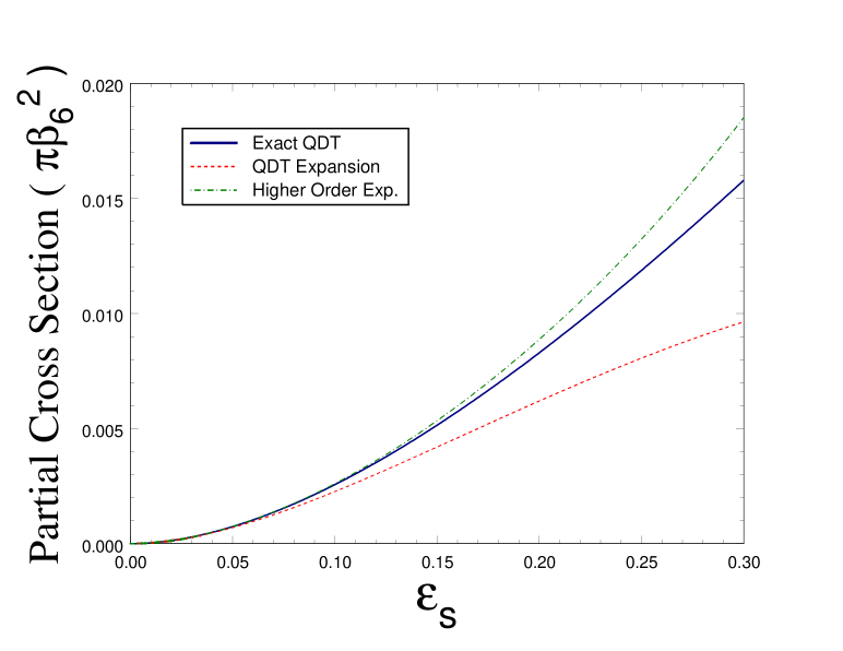
Figure 3: (Color online) $s$ wave partial cross sections for $a_{l=0}=0$, representing the worst-case scenario for the QDT expansion. The results of the recommended QDT expansion (dashed line) are compared to the exact QDT results from Eq. (3) (solid line), and the results of a higher order expansion, given by Eq. (28) (dash-dot line).

Among all partial waves, the QDT expansion for the $s$ wave has the smallest range of applicability because the critical scaled energy, given in Table 2, is smallest for $l=0$. For the $s$ wave, the most stringent test of the expansion is for $a_{l=0}=0$. It corresponds to a case where the lowest order contribution, $-a_{l=0}k$, to $\tan\delta_{l}$ goes to zero, and we are directly testing the higher order terms. As will be discussed in more detail in Sec. IV, this is also the case where the effective range expansion, even in its generalized form of Sec. IV, fails completely. Figure 3 illustrates the accuracy of the QDT expansion for this worst case scenario. It shows that the simpler QDT expansion that we are recommending here is accurate for roughly $\epsilon_{s}<0.1$. From Table 1, it is clear that this range of scaled energies already covers all energies of interest in cold-atom physics. The QDT expansion is more accurate and applicable over a greater range of energies in all other cases and for all other partial waves.

For the $s$ and $p$ partial waves, our results here are consistent with those of Ref. Gao (1998a), except they are now written in simpler forms that are also better for physical interpretation. For $l\geq 2$, the $K^{(D)}$ term, which is of the order of $k_{s}^{2l+1}$ under nonresonant conditions of $|K^{c0}_{l}|$ being of the order of 1 or greater, is normally negligible, as was done in Ref. Gao (1998a). In doing so, however, we missed in our previous work Gao (1998a) the analytic description of low-energy shape resonances for $l\geq 2$, and an opportunity to define the generalized scattering length and the generalized effective range. These subjects are addressed in the next two sections, respectively.

III Threshold behavior of shape resonances

The QDT expansion of Eqs. (29)-(33) is applicable whether or not there is a shape resonance in the threshold region. When such a resonance does exist, which occurs for $l\geq 1$ and a small and negative $K^{c0}_{l}$, namely for $K^{c0}_{l}<0$ and $|K^{c0}_{l}|\ll 1$, further conceptual understanding can be achieved by extracting from the QDT expansion the standard parameters characterizing a resonance, namely its position, width, and background (see, e.g., Ref. Taylor (2006)).

The position of a shape resonance in the threshold region can be determined from the root of the denominator in Eq. (31),

$$\theta_{l}+\pi(\nu-\nu_{0})/2=K^{c0}_{l}\;.$$ (37)

It has solution only for a small and negative $K^{c0}_{l}$, for which it can be solve perturbatively to give the scaled resonance position as

$$\epsilon_{sl}\approx-(2l+3)(2l-1)K^{c0}_{l}\left[1+w_{l}(2l+3)(2l-1)K^{c0}_{l}\right]\;,$$ (38)

in which $w_{l}$ is defined earlier by Eq. (34). Around the shape resonance, the term $K^{(D)}_{l}=-\widetilde{A}_{sl}(\epsilon_{s})k_{s}^{2l+1}$ can be written as

$$K^{(D)}_{l}\approx K^{(D)}_{bgl}(\epsilon_{s})-\frac{1}{2}\frac{\gamma_{sl}}{\epsilon_{s}-\epsilon_{sl}}\;,$$ (39)

with the scaled width, $\gamma_{sl}$, given by

$$\gamma_{sl} \approx 2[(2l+3)(2l-1)]^{l+3/2}\bar{a}_{sl}(-K^{c0}_{l})^{l+1/2}$$ (40)

$$\times\left[1+\frac{3\pi(2l+3)(2l-1)}{4(2l+1)(2l-3)}K^{c0}_{l}\right]\;,$$

$$\approx \frac{2(2l+3)(2l-1)\bar{a}_{sl}(\epsilon_{sl})^{l+1/2}}{1+2w_{l}\epsilon_{sl}}\;,$$ (41)

and the contribution of $K^{(D)}_{l}$ to the background, $K^{(D)}_{bgl}(\epsilon_{s})$, given by

$$K^{(D)}_{bgl=1}\approx-\frac{5\bar{a}_{sl}}{1-\frac{\pi}{7}\epsilon_{sl}}\left(\frac{\epsilon_{s}^{3/2}-\epsilon_{sl}^{3/2}}{\epsilon_{s}-\epsilon_{sl}}\right)-\left(\frac{5\pi}{14}-1\right)\bar{a}_{sl}\epsilon_{s}^{3/2}\;,$$ (42)

$$K^{(D)}_{bgl=2}\approx-\frac{21\bar{a}_{sl}}{1+\frac{\pi}{15}\epsilon_{sl}}\left(\frac{\epsilon_{s}^{5/2}-\epsilon_{sl}^{5/2}}{\epsilon_{s}-\epsilon_{sl}}\right)\;,$$ (43)

$$K^{(D)}_{bgl>2}\approx 0\;.$$ (44)

Corresponding to the width of Eqs. (40) and (41), there is a well-defined lifetime (see, e.g., Ref. Taylor (2006))

$$\tau_{l}=\tau_{sl}s_{T}=(1/\gamma_{sl})s_{T}\;,$$ (45)

where $s_{T}=\hbar/s_{E}$ is the time scale associated with the length scale $\beta_{6}$, with sample values for alkali-metal atoms given in Table 1, and $\tau_{sl}=\tau_{l}/s_{T}=1/\gamma_{sl}$ is the scaled lifetime.

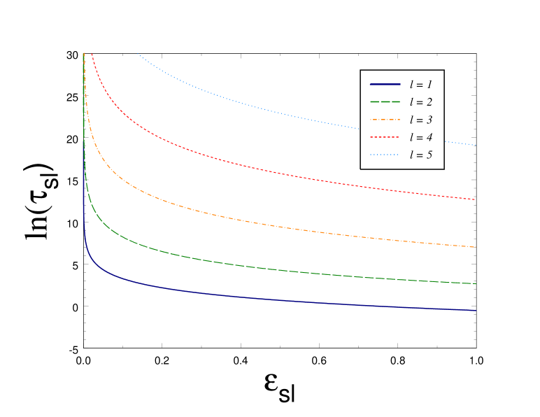
Figure 4: (Color online) Universal relation between the scaled lifetime and the scaled position of a single-channel shape resonance, as given by Eqs. (41) and (45), for $-1/r^{6}$ type of long-range potentials. The lifetime can change by many orders of magnitude for a small change in the resonance position.

Equations (40) and (41) show that the width of a shape resonance goes to zero as it approaches the threshold, below which it becomes a true bound state. The corresponding lifetime goes to infinity. Equation (41) further shows that the scaled width, and therefore the scaled lifetime, when viewed as a function of the scaled resonance position, follows a universal behavior that is uniquely determined by the long-range interaction. In other words, while the resonance position itself, as given by Eq. (38), depends on the short-range parameter $K^{c0}_{l}$, the functional form of the scaled width or lifetime versus the scaled resonance position is independent of it. This universal behavior is illustrated in Figures 4 for the first few partial waves. It also illustrates that the lifetime of a shape resonance can change by many orders of magnitudes, from a microscopic scale of $s_{T}$ (see Table 1), to a macroscopic scale of seconds or longer, as the shape resonance approaches the threshold. The existence of such a potentially macroscopic time scale Knoop et al. (2008) is one of the key differences between the coupling of atoms in $l\neq 0$ and $l=0$ partial waves.

IV Generalized scattering length and generalized effective range

The QDT expansion, Eqs. (29)-(33), already suggests that one may be able to define a generalized scattering length for an arbitrary $l$. This, and the definition of a generalized effective range for an arbitrary $l$, can be done in a way that more closely resembles to the standard ERT Schwinger (1947); Blatt and Jackson (1949); Bethe (1949), as follows.

Defining $\delta^{(B)}_{l}\equiv-\pi(\nu-\nu_{0})$, we have from Eqs. (18)-(22)

$$k_{s}^{2l+1}\cot(\delta_{l}-\delta^{(B)}_{l})=-\left(\frac{1}{\bar{a}_{sl}}\right)\frac{K^{c0}_{l}-\theta_{l}+O(k_{s}^{4})}{1+(-1)^{l}K^{c0}_{l}-[(-1)^{l}-K^{c0}_{l}]\theta_{l}+O(k_{s}^{4})}\left[1+O(k_{s}^{4}\ln k_{s})\right]+O(k_{s}^{4})\;.$$ (46)

In the case of a single channel, the energy dependence of $K^{c0}_{l}$ is completely negligible Gao (1998a, 2001). A further expansion of the denominator in Eq. (46) gives the following generalized effective range expansion

$$k^{2l+1}\cot(\delta_{l}-\delta^{(B)}_{l})=-\frac{1}{\widetilde{a}_{l}}+\frac{1}{2}\widetilde{r}_{el}k^{2}+O(k^{4}\ln k)\;,$$ (47)

with the generalized scattering length, $\widetilde{a}_{l}$, given by

$$\widetilde{a}_{l}=\bar{a}_{l}\left[(-1)^{l}+\frac{1}{K^{c0}_{l}(\epsilon=0)}\right]\;,$$ (48)

where $\bar{a}_{l}=\bar{a}_{sl}\beta_{6}^{2l+1}$ is the mean scattering length for angular momentum $l$ that we have defined earlier (with scale included). The generalized effective range, $\widetilde{r}_{el}$, is given by

$$\widetilde{r}_{el}=-\frac{2\bar{a}_{l}\beta_{6}^{2}}{(2l+3)(2l-1)\widetilde{a}_{l}^{2}}\left\{1+\left[(-1)^{l}-(\widetilde{a}_{l}/\bar{a}_{l})\right]^{2}\right\}\;.$$ (49)

For quantum systems with a long-range $-1/r^{6}$ type of interaction, Eq. (47) defines the generalized scattering length and effective range for an arbitrary $l$. It coincides with standard definitions of scattering lengths and effective ranges whenever they are well defined in the standard theory Schwinger (1947); Blatt and Jackson (1949); Bethe (1949); Levy and Keller (1963). Namely, $\widetilde{a}_{l}=a_{l}$ for $l=0$ and 1, and $\widetilde{r}_{el}=r_{el}$ for $l=0$. Similar to the standard theory, $\widetilde{a}_{l}$ has a dimension of $\beta_{6}^{2l+1}$, and $\widetilde{r}_{el}$ has a dimension of $\beta_{6}^{-2l+1}$. The generalized scattering length is also related to $\widetilde{A}_{sl}(\epsilon_{s})$ by $\widetilde{a}_{l}=\widetilde{A}_{sl}(\epsilon_{s}=0)\beta_{6}^{2l+1}$.

With this definition of generalized scattering length, having a bound or quasibound state right at the threshold, characterized in terms of the $K^{c0}_{l}$ parameter by $K^{c0}_{l}(\epsilon=0)=0$, always corresponds to $\widetilde{a}_{l}=\infty$, for any $l$. Similarly, having a shape resonance close to the threshold, characterized by a small and negative $K^{c0}_{l}$, corresponds to having a large and negative generalized scattering length; having a bound state close to the threshold, characterized by a small and positive $K^{c0}_{l}$, corresponds to having a large and positive generalized scattering length. Such similarities to the $s$-wave interaction make the generalized scattering length an easy parameter to understand, without having to know the QDT behind it. As examples of the generalized scattering lengths for arbitrary $l$, we present, in the Appendix A, their analytic results for two classes of model potentials with $-1/r^{6}$ type of asymptotic behaviors.

We point out that the main utilities of the generalized effective range expansion, Eq. (47), are (a) to define the generalized scattering length as an alternative parameter for describing low-energy atomic interactions, (b) to make a connection between the QDT expansion and the ERT to the degree possible, and (c) to simplify the understanding of the QDT expansion for peoples who are not completely comfortable with QDT formulations. It is not meant to be a replacement for the QDT expansion. As far as accuracy is concerned, the QDT expansion is always more accurate. This loss of accuracy in the generalized ERT occurred in expanding the denominator of Eq. (46), whose full representation would have required an infinite number of terms in the standard ERT type of expansions.

The procedure of expanding the denominator has more severe consequences in the special case of $\widetilde{a}_{l}=0$, for which $\widetilde{r}_{el}=\infty$ from Eq. (49), and the effective range expansion, even in its generalized form here, becomes meaningless. In comparison, the QDT expansion remains applicable, and gives, for $\widetilde{a}_{l}=0$ [corresponding to $K^{c0}_{l}=-(-1)^{l}$],

$$K^{(D)}_{l}\approx\frac{2\bar{a}_{sl}k_{s}^{2l+3}}{(2l+3)(2l-1)-(-1)^{l}k_{s}^{2}-(-1)^{l}w_{l}k_{s}^{4}}\;.$$ (50)

This result also implies that $\widetilde{a}_{l}=0$ changes the threshold behavior of $K_{l}=\tan\delta_{l}$ for $l<2$. For $\widetilde{a}_{l}\neq 0$ (and $\widetilde{a}_{l}\neq\infty$), it is clear from the QDT expansion that the threshold behavior for $l<2$ is determined by the $K^{(D)}_{l}$ term that behaves as $K^{(D)}_{l}\sim-\widetilde{a}_{l}k^{2l+1}$. The threshold behavior for $l\geq 2$ is dominated by the Born term, which behaves as $k_{s}^{4}$. For $\widetilde{a}_{l}=0$, Eq. (50) means that the threshold behavior for the $s$ wave changes from $\tan\delta_{l=0}\sim-\widetilde{a}_{l=0}k$ to $\tan\delta_{l=0}\sim-2\bar{a}_{sl=0}k_{s}^{3}/3$. The threshold behavior for the $p$ wave changes from $\tan\delta_{l=1}\sim-\widetilde{a}_{l=1}k^{3}$ to being dominated by the Born term $\tan\delta_{l=1}\sim-\pi k_{s}^{4}/35$.

Another special case for which the threshold behavior may be modified is the case of $\widetilde{a}_{l}=\infty$ ($K^{c0}_{l}=0$), corresponding to having a bound or quasibound state right at threshold. The QDT expansion gives for this special case

$$K^{(D)}_{l}\approx-\frac{(2l+3)(2l-1)\bar{a}_{sl}k_{s}^{2l-1}}{1+w_{l}k_{s}^{2}}-(-1)^{l}\bar{a}_{sl}k_{s}^{2l+1}\;.$$ (51)

It means, in particular, that the threshold behavior for $\tan\delta_{l}$ is modified for $l\leq 2$ for having a bound or quasibound state right at the threshold. Specifically, it is changed from $\tan\delta_{l}\sim-\widetilde{a}_{l}k^{2l+1}$, for cases of $\widetilde{a}_{l}\neq\infty$ (and $\widetilde{a}_{l}\neq 0$), to $\tan\delta_{l}\sim-(2l+3)(2l-1)\bar{a}_{sl}k_{s}^{2l-1}$ for $\widetilde{a}_{l}=\infty$. The threshold behaviors for $l>2$ remain dominated by the Born term ($\sim k_{s}^{4}$) even with a bound state right at the threshold. We note that the generalized effective range expansion would have given $\widetilde{r}_{el}=-2\beta_{6}^{2}/[(2l+3)(2l-1)\bar{a}_{l}]$ and $\tan\delta_{l}\approx\delta^{(B)}_{l}-(2l+3)(2l-1)\bar{a}_{sl}k_{s}^{2l-1}$ for $\widetilde{a}_{l}=\infty$, corresponding to the lowest order term in Eq. (51).

As a further comment on the generalized effective-range expansion, we note that in arriving at Eq. (49) for the effective range, we have assumed that the energy dependence of $K^{c0}_{l}$ is negligible. This means that Eq. (49) is, strictly speaking, a single channel result that will need to be modified for effective single channel problems where the energy dependence of $K^{c0}_{l}$ is generally important (to be discussed in detail in the companion paper). With this limitation in mind, Eq. (49) does imply that in the case of a single channel, for which the energy dependence of $K^{c0}_{l}$ is negligible, the generalized effective range is not an independent parameter, but can be determined from the generalized scattering length. It further implies that the generalized effective range has the property of $\widetilde{r}_{el}>0$ for $l=0$ and $\widetilde{r}_{el}<0$ for $l\geq 1$, again rigorous only for true single channel problems.

All QDT expansion results of previous two subsections, which were parametrized using $K^{c0}_{l}$, can be written in terms of $\widetilde{a}_{l}$ using Eq. (48), or equivalently,

$$K^{c0}_{l}(\epsilon=0)=\frac{1}{\widetilde{a}_{l}/\bar{a}_{l}-(-1)^{l}}\;.$$ (52)

We do not give these expressions explicitly, in part to again emphasize the following subtle, but important point. The expressions in terms of $K^{c0}_{l}$ are more generally applicable because they make no assumption about the energy dependence of $K^{c0}_{l}$. The corresponding expressions in terms of $\widetilde{a}_{l}$ automatically assumes the weak energy dependence of $K^{c0}_{l}$, since in effect we are using $K^{c0}_{l}(\epsilon=0)$ at other energies. This subtlety is not an issue for true single-channel problems, but becomes one for effective single channel problems derived from multichannel cases (see the companion paper), for which the equations in terms of $K^{c0}_{l}$ remain applicable, but generally not those in terms of $\widetilde{a}_{l}$.

V QDT expansion for bound state energy

The bound spectrum of a two-body, single channel system with $-1/r^{6}$ type of long-range interaction is given rigorously by the solutions of Gao (1998a, 2001, 2008)

$$\chi^{c}_{l}(\epsilon_{s})=K^{c}(\epsilon,l)\;.$$ (53)

where

$$\chi^{c}_{l}(\epsilon_{s})=\frac{\tan\theta_{l}+\tan(\pi\nu/2)(1+M_{\epsilon_{s}l})/(1-M_{\epsilon_{s}l})}{1-\tan\theta_{l}\tan(\pi\nu/2)(1+M_{\epsilon_{s}l})/(1-M_{\epsilon_{s}l})}\;.$$ (54)

is a universal function of $\epsilon_{s}$ that depends only on the exponent of the long-range interaction and on the angular momentum $l$.

For deriving the QDT expansion for the energy of the least-bound state that is close to the threshold, it is again more convenient to rewrite Eq. (53) in terms of the $K^{c0}_{l}$ parameter, as

$$\chi^{c0}_{l}(\epsilon_{s})=K^{c0}_{l}(\epsilon)\;,$$ (55)

where

$$\chi^{c0}_{l}(\epsilon_{s})=\frac{\chi^{c}_{l}(\epsilon_{s})-\tan(\pi\nu_{0}/2)}{1+\tan(\pi\nu_{0}/2)\chi^{c}_{l}(\epsilon_{s})}\;.$$ (56)

Using expansions of $\nu$, $\theta_{l}$, and $M_{\epsilon_{s}l}$, as given by Eqs. (20)-(22), we have, for sufficiently small energies or sufficiently large $l$,

$$\chi^{c0}_{l=0}(\epsilon_{s})\approx\frac{\theta_{l}+\pi(\nu-\nu_{0})/2+\bar{a}_{sl=0}\kappa_{s}-\bar{a}_{sl=0}\kappa_{s}\theta_{l}}{1-\bar{a}_{sl=0}\kappa_{s}-\bar{a}_{sl=0}\kappa_{s}\theta_{l}}\;,$$ (57)

$$\chi^{c0}_{l=1}(\epsilon_{s})\approx\frac{\theta_{l}+\pi(\nu-\nu_{0})/2-\bar{a}_{sl=1}\kappa_{s}^{3}}{1-\bar{a}_{sl=1}\kappa_{s}^{3}}\;,$$ (58)

$$\chi^{c0}_{l\geq 2}(\epsilon_{s})\approx\theta_{l}+\pi(\nu-\nu_{0})/2\;.$$ (59)

Here $\kappa_{s}=(-\epsilon_{s})^{1/2}$, and $\theta_{l}$ and $\pi(\nu-\nu_{0})$ are given by Eqs. (35) and (30), respectively.

Having a bound state of angular momentum $l$ close to the threshold corresponds to having a small and positive $K^{c0}_{l}$. The energy of such a state can be obtained by solving Eq. (55) perturbatively using expansions given by Eqs. (57)-(59). This has been done in Ref. Gao (2004a). We summarize the results here using the standardized notation ($x_{l}$ of Ref. Gao (2004a) is renamed $K^{c0}_{l}$), for the sake of completeness and easy reference.

For the $s$ wave, we obtained

$$\epsilon_{sl=0}=-\frac{1}{\bar{a}_{sl=0}^{2}}(K^{c0}_{l=0})^{2}\left[1+g_{1}K^{c0}_{l=0}+g_{2}(K^{c0}_{l=0})^{2}\right]+O((K^{c0}_{l=0})^{5})\;,$$ (60)

where $\epsilon_{sl}$ is the $l$ wave bound state energy scaled according to Eq. (8), and $g_{1}=2[1/(3\bar{a}_{sl=0}^{2})-1]\approx 0.9179195$, and $g_{2}=(5/4)g_{1}^{2}-2\approx-0.9467798$.

For the $p$ wave, we obtained

$$\epsilon_{sl=1}=-5K^{c0}_{l=1}\left[1+h_{1}(K^{c0}_{l=1})^{1/2}+h_{2}K^{c0}_{l=1}\right]+O((K^{c0}_{l=1})^{5/2})\;,$$ (61)

where $h_{1}=5^{3/2}\bar{a}_{sl=1}\approx 1.299466$, and $h_{2}=3h_{1}^{2}/2-5\pi/14\approx 1.410919$.

For $l\geq 2$, the energy of the least-bound molecular state is given by Eq. (38), namely the same equation that gives the position of the shape resonance above the threshold. This comes from the fact that Eq. (55), with $\chi^{c0}_{l}$ given by Eq. (59), is the same as Eq. (37), which determines the shape resonance positions. The only difference is that while $K^{c0}_{l}$ is small and negative for a shape resonance close to the threshold, it is small and positive for a bound state close to the threshold.

In cases of true single channel problems, these equations can again be written in terms of the generalized scattering length using Eq. (52). The corresponding equations for the $s$ and $p$ waves can be found in Ref. Gao (2004a). We skip writing down these equations explicitly to again emphasize the greater applicability of the equations in terms of $K^{c0}_{l}$. Namely, unlike the equations in terms of the scattering length or generalized scattering length, which assume the energy-independence of $K^{c0}_{l}$, the equations in terms of $K^{c0}_{l}$ are, strictly speaking, applicable even when $K^{c0}_{l}$ itself depends on energy. The only subtlety here is that when the right-hand-sides of equations such as Eqs. (60) and (61) become energy-dependent, they need to be solved again to obtain the bound state energies.

The results presented in this section have been verified in Ref. Gao (2004a) through comparisons with the exact QDT results, obtained by solving Eq. (53) or (55) numerically. The result for the $s$ wave, Eq. (60), has also been verified by Derevianko et al. Derevianko et al. (2009) and by Julienne and Chin Julienne and Chin (2008) through independent numerical calculations. In summary, the formula for the $s$ wave bound state energy is applicable for $a_{l=0}>2\bar{a}_{l=0}$, corresponding, approximately, to $a_{l=0}>\beta_{6}$ or $|\epsilon_{sl=0}|<4$. The formulas for other partial waves are applicable over a greater range of bound state energies Gao (2004a). The intermediate equations, including the expansions of the $\chi^{c0}_{l}$ function as given by Eqs. (57)-(59), and Eq. (55), which is applicable regardless of the energy variations of $K^{c0}_{l}$, will be useful in developing the analytic description of magnetic Feshbach resonance of arbitrary $l$, to be presented in a companion paper.

VI Discussions

We make here some miscellaneous comments on various aspects of the theory, which, while not essential, may be helpful in the understanding of this and related theories.

(a) The QDT expansion breaks naturally into two terms, a Born term $K^{(B)}_{l}$, and a deviation from the Born term $K^{(D)}_{l}$. This separation of $K_{l}=\tan\delta_{l}$ is also convenient for a number of other applications including, e.g, the understanding of angular distribution (see, e.g., Refs. Thomas et al. (2004); Buggle et al. (2004)). There are other separations of $K_{l}=\tan\delta_{l}$ possible. For example, it can be separated into a background term and an interference term, as suggested in Ref. Gao (2008). One can show, however, that these two types of separations are the same for $l>2$, as is reflected in the fact that the $K^{(D)}_{l}$ term has negligible contribution to the background for $l>2$ [see Eqs. (39) and (44)].

(b) Unlike the cases of $s$ and $p$ partial waves, the generalized scattering length for $l\geq 2$ has little effect on scattering cross sections around the threshold, except in determining the location of the shape resonance, and if there is one, the cross sections around it.

(c) For true single channel problems, having an ultracold shape resonance can only happen by accident. In this sense, the most important applications of a theory for ultracold shape resonance are not to the true single channel problems, but to the effective single channel problems associated with Feshbach resonances, for which there will be at least one state in the threshold region as the Feshbach resonance is tuned around it. It is for this reason that we kept stressing the formulas that remain applicable when $K^{c0}_{l}$ becomes energy-dependent, which is the single most important difference between an effective single channel problem for a Feshbach resonance, and a true single channel problem.

It is for the same reason that we did not emphasize the relationship of $K^{c0}_{l}$ for different $l$. For a true single channel problem, the $K^{c0}_{l}$ parameter for different $l$ are not independent, but are related to each other through Eq. (9), in which $K^{c}$ is approximately independent of $l$ Gao (2001). As a result, the $K^{c0}_{l}$ for the first few partial wave can all be determined from, e.g., the $s$ wave scattering length. This simple relationship between different $l$ breaks down for the effective single channel problems for Feshbach resonances. For such intrinsically multichannel problems, the $K^{c0}_{l}$ parameters for different $l$ are still related, as the underlying short-range $K^{c}$ matrix is still approximately $l$-independent. Their values for different $l$ can still be computed from, e.g., the singlet and the triplet $s$ wave scattering length for alkali-metal atoms Gao et al. (2005). Their relationship, however, becomes more complicated than Eq. (9) and less transparent.

(d) While we have no intention of promoting one parameter over the other, as they all have different utilities, we hope this work again illustrates that the scattering length, or the generalized scattering length, is not the only parameter, or necessarily the best parameter for characterizing atomic interaction at low temperatures. While many of our results, such as those for resonance positions and binding energies, can be written in terms of the scattering length or the generalized scattering length, such equations are more complex than those in terms of $K^{c0}_{l}$, and have more restricted applicability to the case of single channel. Furthermore, it should be clear that in the scattering length representation, what is important is not the scattering length itself, but the dimensionless ratio $\widetilde{a}_{l}/\bar{a}_{l}$, as is also recognized by Chin et. al Chin et al. (2008) for the $s$ wave.

(e) We point out that there are a number of other successful QDT formulations of atomic interaction that are conceptually similar to ours in many aspects, but based on numerical reference functions Mies (1984); Mies and Julienne (1984); Julienne and Mies (1989); Burke, Jr. et al. (1998); Mies and Raoult (2000); Raoult and Mies (2004). Without incorporating at least some ingredients of an analytic solution, numerical solutions generally run into difficulty for very large scattering lengths, namely when there is a state very close to the threshold. This is true for the $s$ wave Julienne (2008), and more so for higher partial waves.

VII Conclusions

In conclusion, we have presented an analytic description of atomic interactions at ultracold temperatures for the case of single channel. In particular, a QDT expansion for scattering has been developed that is applicable to all angular momentum $l$, with or without the presence of ultracold shape resonances. Using the QDT expansion, we have developed a fully analytic characterization of ultracold shape resonances in terms of its position, width, and background. We have also introduced a generalized scattering length that can be used as an alternative parameter to characterize atomic interaction at low temperatures, and discussed the changes of threshold behaviors in the special cases of zero and infinite generalized scattering lengths. The analytic formulas derived make it possible for an accurate description of atomic interaction in the ultracold regime without having to know the details of the QDT or resort to numerical calculations.

The generalities of the results of this work will further manifest themselves in a companion work on atomic interaction around a magnetic Feshbach resonance, which is necessarily multichannel in nature Tiesinga et al. (1993); Köhler et al. (2006); Chin et al. (2008). We will show that such a multichannel problem can be rigorously reduced to an effective single channel problem, to which most of our results here remain applicable. The key difference will be that the effective $K^{c0}_{l}$ parameter becomes energy dependent. It is this energy dependence that leads to deviations from the single channel universal behaviors that correspond to the results here specialized to an energy-independent $K^{c0}_{l}$.

*

Appendix A Analytic results of $K^{c0}_{l}$ and generalized scattering lengths for two type of model potentials

In a previous work Gao (2003), we have derived, for two classes of model potentials, the analytic results of $K^{c}(\epsilon=0,l)$ and the number of bound states $N_{l}$ for an arbitrary $l$. One class, denoted by HST$n$, is of the type of a hard-sphere with an attractive tail:

$$V_{\text{HST}n}(r)=\left\{\begin{array}[]{lcl}\infty&,&r\leq r_{0}\\ -C_{n}/r^{n}&,&r>r_{0}\end{array}\right.\;.$$ (62)

The other, denoted by LJ$n$, is of the type of Lennard-Jones LJ$(n,2n-2)$:

$$V_{\text{LJ}n}(r)=-C_{n}/r^{n}+C_{2n-2}/r^{2n-2}\;,$$ (63)

which corresponds, in particular, to a LJ(6,10) potential for $n=6$.

For HST$n$ potentials, we have shown that the $K^{c}$ parameter at zero energy is given by Gao (2003)

$$K_{\text{HST}n}^{c}(0,l)=-\frac{J_{\nu_{0}}(y_{0})\cos(\pi\nu_{0}/2)-Y_{\nu_{0}}(y_{0})\sin(\pi\nu_{0}/2)}{J_{\nu_{0}}(y_{0})\sin(\pi\nu_{0}/2)+Y_{\nu_{0}}(y_{0})\cos(\pi\nu_{0}/2)},$$ (64)

where $\nu_{0}=(2l+1)/(n-2)$, $J$ and $Y$ are the Bessel functions Abramowitz and Stegun (1964), and $y_{0}=[2/(n-2)](\beta_{n}/r_{0})^{(n-2)/2}$, in which $\beta_{n}=(2\mu C_{n}/\hbar^{2})^{1/(n-2)}$ is the length scale associated with the $C_{n}/r^{n}$ type of potentials.

For LJ$n$ potentials, we have derived Gao (2003)

$$K_{\text{LJ}n}^{c}(0,l)=\tan(\pi\nu_{0}/2)[1+h_{l}(z_{0})][1-h_{l}(z_{0})]^{-1},$$ (65)

where $z_{0}=(\beta_{n}/\beta_{2n-2})^{n-2}/[2(n-2)]$ and

$$h_{l}(z_{0})=z_{0}^{\nu_{0}}\frac{\sin\pi(z_{0}+1/2-\nu_{0}/2)\Gamma(z_{0}+1/2-\nu_{0}/2)}{\sin\pi(z_{0}+1/2+\nu_{0}/2)\Gamma(z_{0}+1/2+\nu_{0}/2)}\;.$$ (66)

Substituting these results into Eq. (9), We obtain

$$K^{c0}_{l}(\epsilon=0)=-J_{\nu_{0}}(y_{0})/Y_{\nu_{0}}(y_{0})\;,$$ (67)

for HST$n$ potentials, and

$$K^{c0}_{l}(\epsilon=0)=\frac{\sin(\pi\nu_{0})h_{l}(z_{0})}{1-\cos(\pi\nu_{0})h_{l}(z_{0})}\;,$$ (68)

for LJ$n$ potentials. Both results are applicable for arbitrary $n$ and $l$.

Specializing to the case of $n=6$, these results, combined with QDT for $n=6$ Gao (1998a, 2001, 2008), provide an accurate description of the scattering and bound state properties for these model potentials over a wide range of energies around the threshold. They also give us the analytic results of the generalized scattering length for an arbitrary $l$. From Eq. (48), we have, for $n=6$,

$$\widetilde{a}_{l}=\bar{a}_{l}\left[(-1)^{l}-Y_{\nu_{0}}(y_{0})/J_{\nu_{0}}(y_{0})\right]\;,$$ (69)

for HST6 potential, where $\nu_{0}=(2l+1)/4$ and $y_{0}=(\beta_{6}/r_{0})^{2}/2$, and

$$\widetilde{a}_{l}=\frac{\bar{a}_{l}}{\sin(\pi\nu_{0})h_{l}(z_{0})}\;,$$ (70)

for LJ6 potential, where $z_{0}=(\beta_{6}/\beta_{10})^{4}/8$. The generalized effective range can be derived from these results using Eq. (49). If one specializes Eq. (69) to $l=0$, one recovers, for the HST6 potential, the result of Gribakin and Flambaum Gribakin and Flambaum (1993) for the $s$ wave.

The analytic results of this Appendix are useful for designing model potentials to investigate universal properties not only in two-body Gao (2003, 2004b), but also in few-body and many-body quantum systems Gao (2003, 2004c); Khan and Gao (2006). They can also be used to check the accuracies of various numerical techniques and methods. Last but not the least, they give an explicit illustration of one of the important properties of $K^{c}$ and related parameters, i.e., $K^{c}(\epsilon,l)$, and therefore $K^{c0}_{l}(\epsilon=0)$ and $\widetilde{a}_{l}$, are meromorphic functions of $l$, namely, they are analytic functions of $l$ with only simple poles Gao (2008).

References

- Tiesinga et al. (1993) E. Tiesinga, B. J. Verhaar, and H. T. C. Stoof, Phys. Rev. A 47, 4114 (1993).
- Köhler et al. (2006) T. Köhler, K. Góral, and P. S. Julienne, Rev. Mod. Phys. 78, 1311 (2006).
- Chin et al. (2008) C. Chin, R. Grimm, P. S. Julienne, and E. Tiesinga, arXiv:0812.1496 (2008).
- Regal et al. (2003) C. A. Regal, C. Ticknor, J. L. Bohn, and D. S. Jin, Phys. Rev. Lett. 90, 053201 (2003).
- Ticknor et al. (2004) C. Ticknor, C. A. Regal, D. S. Jin, and J. L. Bohn, Phys. Rev. A 69, 042712 (2004).
- Zhang et al. (2004) J. Zhang, E. G. M. van Kempen, T. Bourdel, L. Khaykovich, J. Cubizolles, F. Chevy, M. Teichmann, L. Tarruell, S. J. J. M. F. Kokkelmans, and C. Salomon, Phys. Rev. A 70, 030702 (2004).
- Schunck et al. (2005) C. H. Schunck, M. W. Zwierlein, C. A. Stan, S. M. F. Raupach, W. Ketterle, A. Simoni, E. Tiesinga, C. J. Williams, and P. S. Julienne, Phys. Rev. A 71, 045601 (2005).
- Gaebler et al. (2007) J. P. Gaebler, J. T. Stewart, J. L. Bohn, and D. S. Jin, Phys. Rev. Lett. 98, 200403 (2007).
- Knoop et al. (2008) S. Knoop, M. Mark, F. Ferlaino, J. G. Danzl, T. Kraemer, H.-C. Nägerl, and R. Grimm, Phys. Rev. Lett. 100, 083002 (2008).
- Moerdijk et al. (1995) A. J. Moerdijk, B. J. Verhaar, and A. Axelsson, Phys. Rev. A 51, 4852 (1995).
- Schwinger (1947) J. Schwinger, Phys. Rev. 72, 738 (1947).
- Blatt and Jackson (1949) J. M. Blatt and D. J. Jackson, Phys. Rev. 76, 18 (1949).
- Bethe (1949) H. A. Bethe, Phys. Rev. 76, 38 (1949).
- Levy and Keller (1963) B. R. Levy and J. B. Keller, J. Math. Phys. 4, 54 (1963).
- Gao (1998a) B. Gao, Phys. Rev. A 58, 4222 (1998a).
- Williams (1945) E. J. Williams, Rev. Mod. Phys. 17, 217 (1945).
- Kirschner and Le Roy (1978) S. M. Kirschner and R. J. Le Roy, J. Chem. Phys. 68, 3139 (1978).
- Julienne and Mies (1989) P. S. Julienne and F. H. Mies, J. Opt. Soc. Am. B 6, 2257 (1989).
- Gribakin and Flambaum (1993) G. F. Gribakin and V. V. Flambaum, Phys. Rev. A 48, 546 (1993).
- Trost et al. (1998a) J. Trost, C. Eltschka, and H. Friedrich, J. Phys. B 31, 361 (1998a).
- Boisseau et al. (1998) C. Boisseau, E. Audouard, and J. Vigué, Europhys. Lett. 41, 349 (1998).
- Trost et al. (1998b) J. Trost, C. Eltschka, and H. Friedrich, Europhys. Lett. 43, 230 (1998b).
- Flambaum et al. (1999) V. V. Flambaum, G. F. Gribakin, and C. Harabati, Phys. Rev. A 59, 1998 (1999).
- Gao (1999) B. Gao, Phys. Rev. Lett. 83, 4225 (1999).
- Gao (2008) B. Gao, Phys. Rev. A 78, 012702 (2008).
- Gao (2001) B. Gao, Phys. Rev. A 64, 010701(R) (2001).
- Gao (2004a) B. Gao, J. Phys. B 37, 4273 (2004a).
- Gao et al. (2005) B. Gao, E. Tiesinga, C. J. Williams, and P. S. Julienne, Phys. Rev. A 72, 042719 (2005).
- Gao (1998b) B. Gao, Phys. Rev. A 58, 1728 (1998b).
- Yan et al. (1996) Z.-C. Yan, J. F. Babb, A. Dalgarno, and G. W. F. Drake, Phys. Rev. A 54, 2824 (1996).
- Derevianko et al. (1999) A. Derevianko, W. R. Johnson, M. S. Safronova, and J. F. Babb, Phys. Rev. Lett. 82, 3589 (1999).
- Marte et al. (2002) A. Marte, T. Volz, J. Schuster, S. Dürr, G. Rempe, E. G. M. van Kempen, and B. Verhaar, Phys. Rev. Lett. 89, 283202 (2002).
- Claussen et al. (2003) N. R. Claussen, S. J. J. M. F. Kokkelmans, S. T. Thompson, E. A. Donley, E. Hodby, and C. E. Wieman, Phys. Rev. A 67, 060701(R) (2003).
- Chin et al. (2004) C. Chin, V. Vuletić, A. J. Kerman, S. Chu, E. Tiesinga, P. J. Leo, and C. J. Williams, Phys. Rev. A 70, 032701 (2004).
- Gao (2000) B. Gao, Phys. Rev. A 62, 050702(R) (2000).
- Gao (2004b) B. Gao, Euro. Phys. J. D 31, 283 (2004b).
- Abramowitz and Stegun (1964) M. Abramowitz and I. A. Stegun, eds., Handbook of Mathematical Functions (National Bureau of Standards, Washington, D.C., 1964).
- Landau and Lifshitz (1977) L. D. Landau and E. M. Lifshitz, Quantum Mechanics (Pergamon Press, Oxford, 1977).
- Chen and Gao (2007) Y. Chen and B. Gao, Phys. Rev. A 75, 053601 (2007).
- Taylor (2006) J. R. Taylor, Scattering Theory (Dover Publications, Mineola, New York, 2006).
- Derevianko et al. (2009) A. Derevianko, E. Luc-Koenig, and F. Masnou-Seeuws, Can. J. Phys. 87, 67 (2009).
- Julienne and Chin (2008) P. S. Julienne and C. Chin (2008), private communications.
- Thomas et al. (2004) N. R. Thomas, N. Kjærgaard, P. S. Julienne, and A. C. Wilson, Phys. Rev. Lett. 93, 173201 (2004).
- Buggle et al. (2004) C. Buggle, J. Léonard, W. von Klitzing, and J. T. M. Walraven, Phys. Rev. Lett. 93, 173202 (2004).
- Mies (1984) F. H. Mies, J. Chem. Phys. 80, 2514 (1984).
- Mies and Julienne (1984) F. H. Mies and P. S. Julienne, J. Chem. Phys. 80, 2526 (1984).
- Burke, Jr. et al. (1998) J. P. Burke, Jr., C. H. Greene, and J. L. Bohn, Phys. Rev. Lett. 81, 3355 (1998).
- Mies and Raoult (2000) F. H. Mies and M. Raoult, Phys. Rev. A 62, 012708 (2000).
- Raoult and Mies (2004) M. Raoult and F. H. Mies, Phys. Rev. A 70, 012710 (2004).
- Julienne (2008) P. S. Julienne (2008), private communications.
- Gao (2003) B. Gao, J. Phys. B 36, 2111 (2003).
- Gao (2004c) B. Gao, J. Phys. B 37, L227 (2004c).
- Khan and Gao (2006) I. Khan and B. Gao, Phys. Rev. A 73, 063619 (2006).