Exact solutions and stability of rotating dipolar Bose-Einstein condensates in the Thomas-Fermi limit

Abstract

We present a theoretical analysis of dilute gas Bose-Einstein condensates with dipolar atomic interactions under rotation in elliptical traps. Working in the Thomas-Fermi limit, we employ the classical hydrodynamic equations to first derive the rotating condensate solutions and then consider their response to perturbations. We thereby map out the regimes of stability and instability for rotating dipolar Bose-Einstein condensates and in the latter case, discuss the possibility of vortex lattice formation. We employ our results to propose several novel routes to induce vortex lattice formation in a dipolar condensate.

I Introduction

The successful Bose-Einstein condensation of ⁵²Cr atoms Griesmaier05 ; Lahaye07 ; Koch08 realizes for the first time Bose-Einstein condensates (BECs) with significant dipole-dipole interactions. These long-range and anisotropic interactions introduce rich physical effects, as well as new opportunities to control BECs. A basic example is how dipole-dipole interactions modify the shape of a trapped BEC. In a prolate (elongated) dipolar gas with the dipoles polarised along the long axis the net dipolar interaction is attractive, whereas for an oblate (flattened) configuration with the dipoles aligned along the short axis the net dipolar interaction is repulsive. As a result, in comparison to s-wave BECs (which we define as systems in which atom-atom scattering is dominated by the s-wave channel), a dipolar BEC elongates along the direction of an applied polarizing field Santos00 ; Yi01 .

A full theoretical treatment of a trapped BEC involves solving the Gross-Pitaevskii equation (GPE) for the condensate wave function Pethick&Smithbook ; Pitaevskii&StringariBook . The non-local nature of the mean-field potential describing dipole-dipole interactions means that this task is significantly harder for dipolar BECs than for s-wave ones. However, in the limit where the BEC contains a large number of atoms the problem of finding the ground state density profile and low-energy dynamics simplifies. In a harmonic trap with oscillator length $a_{\mathrm{ho}}=\sqrt{\hbar/(m\omega)}$, a BEC containing $N$ atoms of mass $m$ which have repulsive s-wave interactions characterized by scattering length $a$ enters the Thomas-Fermi (TF) regime for large values of the parameter $Na/a_{\mathrm{ho}}$ Pethick&Smithbook ; Pitaevskii&StringariBook . In the TF regime the zero-point kinetic energy can be ignored in comparison to the interaction and trapping energies and the Gross-Pitaevskii equation reduces to the equations of superfluid hydrodynamics at $T=0$ Pethick&Smithbook ; Pitaevskii&StringariBook ; Pines&NozieresBook . When applied to a trapped $s$-wave BEC these equations are known to admit a large class of exact analytic solutions stringari96 . The TF approximation can also be applied to dipolar BECs Parker08 . Although the resulting superfluid hydrodynamic equations for a dipolar BEC contain the non-local dipolar potential, exact solutions can still be found ODell04 ; Eberlein05 and we make extensive use of them here. The calculations in this paper are all made within the TF regime.

Condensates are quantum fluids described by a macroscopic wave function $\psi=\sqrt{\rho}\exp[\mathrm{i}S]$, where $\rho$ is the condensate density and $S$ is the condensate phase. This constrains the velocity field $\underline{v}=(\hbar/m)\underline{\nabla}S$ to be curl-free $\underline{\nabla}\times\underline{v}=0$. In an experiment rotation of the condensate can be accomplished by applying a rotating elliptical deformation to the trapping potential Madison00 ; Hodby02 . At low rotation frequencies the elliptical deformation excites low-lying collective modes (quadrupole etc.) with quantized angular momentum which may be viewed as surface waves (and which obey $\underline{\nabla}\times\underline{v}=0$). Above a certain critical rotation frequency vortices are seen to enter the condensate and these satisfy the $\underline{\nabla}\times\underline{v}=0$ condition by having quantized circulation. The hydrodynamic equations for a BEC provide a simple and accurate description of the low-lying collective modes. Furthermore, they predict these modes become unstable for certain ranges of rotation frequency Recati01 ; Sinha01 . Comparison with experiments Madison00 ; Hodby02 and full numerical simulations of the GPE Lundh03 ; Parker06 ; Corro07 have clearly shown that the instabilities are the first step in the entry of vortices into the condensate and the formation of a vortex lattice. Crucially, the hydrodynamic equations give a clear explanation of why vortex lattice formation in $s$-wave BECs was only observed to occur at a much greater rotation frequency than that at which they become energetically favorable. It is only at these higher frequencies that the vortex-free condensate becomes dynamically unstable.

Individual vortices Pu06 ; ODell07 ; Wilson08 and vortex lattices Cooper05 ; Zhang05 ; Cooper07 in dipolar condensates have already been studied theoretically. However, a key question that remains is how to make such states in the first place. In this paper we extend the TF approximation for rotating trapped condensates to include dipolar interactions, building on our previous work Bijnen07 ; Martin08 . Specifically, starting from the hydrodynamic equations of motion we obtain the stationary solutions for a condensate in a rotating elliptical trap and find when they become dynamically unstable to perturbations. This enables us to predict the regimes of stable and unstable motion of a rotating dipolar condensate. For a non-dipolar BEC (in the TF limit) the transition between stable and unstable motion is independent of the interaction strength, and depends only on the rotation frequency and trap ellipticity in the plane perpendicular to the rotation vector Recati01 ; Sinha01 . We show that for a dipolar BEC it is additionally dependent on the strength of the dipolar interactions and also the axial trapping strength. All of these quantities are experimentally tunable and this extends the routes that can be employed to induce instability. Meanwhile, the critical rotation frequency at which vortices become energetically favorable $\Omega_{v}$ is also sensitive to the trap geometry and dipolar interactions ODell07 , and means that the formation of a vortex lattice following the instability cannot be assumed. Using a simple prediction for this frequency, we indicate the regimes in which we expect vortex lattice formation to occur. By considering all of the key and experimentally tunable quantities in the system we outline several accessible routes to generate instability and vortex lattices in dipolar condensates.

This paper is structured as follows. In Section II we introduce the mean-field theory and the TF approximation for dipolar BECs, in Section III we derive the hydrodynamic equations for a trapped dipolar BEC in the rotating frame, and in Section IV we obtain the corresponding stationary states and discuss their behaviour. In Section V we show how to obtain the dynamical stability of these states to perturbations, and in Section VI we employ the results of the previous sections to discuss possible pathways to induce instability in the motion of the BEC and discuss the possibility that such instability leads to the formation of a vortex lattice. Finally in Section VII we conclude our findings and suggest directions for future work.

II Mean-field theory of a dipolar BEC

We consider a BEC with long-range dipolar atomic interactions, with the dipoles aligned in the $z$ direction by an external field. The condensate wave function (mean-field order parameter) for the condensate $\psi\equiv\psi(\underline{r},t)$ satisfies the GPE which is given by Goral00 ; Santos00 ; Yi00 ,

$$i\hbar\frac{\partial\psi}{\partial t}=\left[-\frac{\hbar^{2}}{2m}\nabla^{2}+V(\underline{r},t)+\Phi_{dd}(\underline{r},t)+g\left|\psi\right|^{2}\right]\psi,$$

where $m$ is the atomic mass. The $\nabla^{2}$-term arises from kinetic energy and $V(\underline{r},t)$ is the external confining potential. BECs typically feature s-wave atomic interactions which gives rise to a local cubic nonlinearity with coefficient $g=4\pi\hbar^{2}a/m$, where $a$ is the s-wave scattering length. Note that $a$, and therefore $g$, can be experimentally tuned between positive values (repulsive interactions) and negative values (attractive interactions) by means of a Feshbach resonance Lahaye07 ; Koch08 . The dipolar interactions lead to a non-local mean-field potential $\Phi_{dd}(\underline{r},t)$ which is given by Yi01 ,

$$\Phi_{dd}(\underline{r},t)=\int d^{3}r~{}U_{dd}\left(\underline{r}-\underline{r}^{\prime}\right)\rho\left(\underline{r}^{\prime},t\right),$$ (2)

where $\rho(\underline{r},t)=|\psi(\underline{r},t)|^{2}$ is the condensate density and

$$U_{dd}(\underline{r})=\frac{C_{dd}}{4\pi}\frac{1-3\cos^{2}\theta}{|\underline{r}|^{3}}$$ (3)

is the interaction potential of two dipoles separated by a vector $\underline{r}$, where $\theta$ is the angle between $\underline{r}$ and the polarization direction, which we take to be the $z$-axis. The dipolar BECs made to date have featured permanent magnetic dipoles. Then, assuming the dipoles to have moment $d_{m}$ and be aligned in an external magnetic field $\underline{B}=\hat{k}B$, the dipolar coupling is $C_{dd}=\mu_{0}d_{m}^{2}$ Goral00 , where $\mu_{0}$ is the permeability of free space. Alternatively, for dipoles induced by a static electric field $\underline{E}=\hat{k}E$, the coupling constant $C_{dd}=E^{2}\alpha^{2}/\epsilon_{0}$ Yi00 ; You98 , where $\alpha$ is the static polarizability and $\epsilon_{0}$ is the permittivity of free space. In both cases, the sign and magnitude of $C_{dd}$ can be tuned through the application of a fast-rotating external field Giovanazzi02 .

We will specify the interaction strengths through the parameter

$$\varepsilon_{dd}=\frac{C_{dd}}{3g},$$ (4)

which is the ratio of the dipolar interactions to the s-wave interactions Giovanazzi02 . We take the s-wave interactions to be repulsive, $g>0$, and so where we discuss negative values of $\varepsilon_{dd}$, this corresponds to $C_{dd}<0$. We will also limit our analysis to the regime of $-0.5<\varepsilon_{dd}<1$, where the Thomas-Fermi approach predicts that non-rotating stationary solutions are robustly stable ODell04 . Outside of this regime the situation becomes more complicated since the non-rotating system becomes prone to collapse Parker09 .

We are concerned with a BEC confined by an elliptical harmonic trapping potential of the form,

$$V(\underline{r})=\frac{1}{2}m\omega_{\perp}^{2}\left[(1-\epsilon)x^{2}+(1+\epsilon)y^{2}+\gamma^{2}z^{2}\right].$$ (5)

In the $x-y$ plane the trap has mean trap frequency $\omega_{\perp}$ and ellipticity $\epsilon$. The trap strength in the axial direction, and indeed the geometry of the trap itself, is specified by the trap ratio $\gamma=\omega_{z}/\omega_{\perp}$. When $\gamma\gg 1$ the BEC shape will typically be oblate (flattened) while for $\gamma\ll 1$ it will typically be prolate (elongated), although for strong enough dipolar interactions the electrostrictive/magnetostrictive effect can cause a BEC in an oblate trap to become prolate itself.

The time-dependent GPE (II) can be reduced to its time-independent form by making the substitution $\psi(\underline{r},t)=\sqrt{\rho(\underline{r})}\exp(i\mu t/\hbar)$, where $\mu$ is the chemical potential of the system. We employ the TF approximation whereby the kinetic energy of static solutions is taken to be negligible in comparison to the potential and interaction energies. The validity of this approximation in dipolar BECs has been discussed elsewhere Parker08 . Then, the time-independent GPE reduces to,

$$V(\underline{r})+\Phi_{dd}(\underline{r})+g\rho(\underline{r})=\mu.$$ (6)

For ease of calculation the dipolar potential $\Phi_{dd}(\underline{r})$ can be expressed as,

$$\Phi_{dd}(\underline{r})=-3g\varepsilon_{dd}\left(\frac{\partial^{2}}{\partial z^{2}}\phi(\underline{r})+\frac{1}{3}\rho(\underline{r})\right),$$ (7)

where $\phi(\underline{r})$ is a fictitious ‘electrostatic’ potential defined by ODell04 ; Eberlein05 ,

$$\phi(\underline{r})=\frac{1}{4\pi}\int\frac{d^{3}r^{\prime}\rho(\underline{r}^{\prime})}{\left|\underline{r}-\underline{r}^{\prime}\right|}.$$ (8)

This effectively reduces the problem of calculating the dipolar potential (2) to the calculation of an electrostatic potential of the form (8), for which a much larger theoretical body of literature exists. Exact solutions of Eq. (6) for $\rho(\underline{r})$, $\phi(\underline{r})$ and hence $\Phi_{dd}(\underline{r})$ can be obtained for any general parabolic trap, as proven in Appendix A of Ref. Eberlein05 . In particular, the solutions of $\rho(\underline{r})$ take the form

$$\rho(\underline{r})=\rho_{0}\left(1-\frac{x^{2}}{R_{x}^{2}}-\frac{y^{2}}{R_{y}^{2}}-\frac{z^{2}}{R_{z}^{2}}\right)\,\,\,\,{\rm for}\,\,\,\rho(\underline{r})\geq 0$$ (9)

where $\rho_{0}=15N/(8\pi R_{x}R_{y}R_{z})$ is the central density. Remarkably, this is the general inverted parabola density profile familiar from the TF limit of non-dipolar BECs. An important distinction, however, is that for the dipolar BEC the aspect ratio of the parabolic solution differs from the trap aspect ratio.

III Hydrodynamic Equations in the Rotating Frame

Having introduced the TF model of a dipolar BEC we now extend this to include rotation and derive hydrodynamic equations for the rotating system. We consider the rotation to act about the $z$-axis, described by the rotation vector $\underline{\Omega}$ where $\Omega=|\underline{\Omega}|$ is the rotation frequency and the Hamiltonian in the rotating frame is given by,

$$H_{{\rm eff}}=H_{0}-\underline{\Omega}\cdot\hat{L},$$ (10)

where $H_{0}$ is the Hamiltonian in absence of the rotation and $\hat{L}=-i\hbar(\underline{r}\times\underline{\nabla})$ is the quantum mechanical angular momentum operator. Using this result with the Hamiltonian $H_{0}$ from Eq. (II) we obtain Leggett_Book ; Leggett00 ,

$$i\hbar\frac{\partial\Psi(\underline{r},t)}{\partial t} = \left[-\frac{\hbar^{2}}{2m}\nabla^{2}+V(\underline{r})+\Phi_{dd}(\underline{r},t)+g|\Psi(\underline{r},t)|^{2}\right.$$ (11)

$$- \left.\Omega\frac{\hbar}{i}\left(x\frac{\partial}{\partial y}-y\frac{\partial}{\partial x}\right)\right]\Psi(\underline{r},t).$$

Note that all space coordinates $\underline{r}$ are those of the rotating frame and the time independent trapping potential $V(\underline{r})$, given by Eq. (5), is stationary in this frame. Momentum coordinates, however, are expressed in the laboratory frame Leggett_Book ; Leggett00 ; Lifshitz .

We can express the condensate mean field in terms of a density $\rho(\underline{r},t)$ and phase $S(\underline{r},t)$ as $\psi(\underline{r},t)=\sqrt{\rho(\underline{r},t)}\exp[iS(\underline{r},t)]$, and so that the condensate velocity is $\underline{v}=(\hbar/m)\underline{\nabla}S$. Substuting into the time-dependent GPE (11) and equating imaginary and real terms leads to the following equations of motion,

$$\frac{\partial\rho}{\partial t} = -\underline{\nabla}\cdot\left[\rho\left(\underline{v}-\underline{\Omega}\times\underline{r}\right)\right],$$ (12)

$$m\frac{\partial\underline{v}}{\partial t} = -\underline{\nabla}\left(\frac{1}{2}m\underline{v}\cdot\underline{v}+V(\underline{r})+\Phi_{dd}(\underline{r})\right.$$ (13)

$$+\left.g\rho-m\underline{v}\cdot\left[\underline{\Omega}\times\underline{r}\right]\right).$$

In the absence of dipolar interactions ($\Phi_{dd}=0$) Eqs. (12) and (13) are commonly known as the superfluid hydrodynamic equations Pethick&Smithbook ; Pitaevskii&StringariBook ; Pines&NozieresBook since they resemble the equation of continuity and the Euler equation of motion from dissipationless fluid dynamics. Here we have extended them to include dipolar interactions.

Note that the form of condensate velocity leads to the relation,

$$\underline{\nabla}\times\underline{v}=\frac{\hbar}{m}\underline{\nabla}\times\underline{\nabla}S=0,$$ (14)

which immediately reveals that the condensate is irrotational. The exceptional case is when the velocity potential $(\hbar/m)S$ is singular, which arises when a quantized vortex occurs in the system.

IV Stationary Solution of the Hydrodynamic Equations

We now search for stationary solutions of the hydrodynamic Eqs. (12) and (13). These states satisfy the equilibrium conditions,

$$\frac{\partial\rho}{\partial t}=0,\hskip 56.9055pt\frac{\partial\underline{v}}{\partial t}=0.$$ (15)

Following the approach of Recati et al. Recati01 we assume the velocity field ansatz,

$$\underline{v}=\alpha\underline{\nabla}(xy).$$ (16)

Here $\alpha$ is a velocity field amplitude that will provide us with a key parameter to parameterise our rotating solutions. Note that this is the velocity field in the laboratory frame expressed in the coordinates of the rotating frame, and also that it satisfies the irrotationality condition (14). Combining Eqs. (13) and (16) we obtain the relation,

$$\mu=\frac{m}{2}\left(\tilde{\omega}_{x}^{2}x^{2}+\tilde{\omega}_{y}^{2}y^{2}+\omega_{z}^{2}z^{2}\right)+g\rho(\underline{r})+\Phi_{dd}(\underline{r}),$$ (17)

where the effective trap frequencies $\tilde{\omega}_{x}$ and $\tilde{\omega}_{y}$ are given by,

$$\tilde{\omega}_{x}^{2}=\omega_{\perp}^{2}(1-\epsilon)+\alpha^{2}-2\alpha\Omega$$ (18)

$$\tilde{\omega}_{y}^{2}=\omega_{\perp}^{2}(1+\epsilon)+\alpha^{2}+2\alpha\Omega.$$ (19)

The dipolar potential inside an inverted parabola density profile (9) has been found in Refs. Eberlein05 ; Bijnen07 to be,

$$\frac{\Phi_{dd}}{3g\varepsilon_{dd}} = \frac{\rho_{0}\kappa_{x}\kappa_{y}}{2}\left[\beta_{001}-\frac{x^{2}\beta_{101}+y^{2}\beta_{011}+3z^{2}\beta_{002}}{R_{z}^{2}}\right]-\frac{\rho}{3}$$

where we have defined the condensate aspect ratios $\kappa_{x}=R_{x}/R_{z}$ and $\kappa_{y}=R_{y}/R_{z}$, and where the coefficients $\beta_{ijk}$ are given by,

$$\beta_{ijk}=\int_{0}^{\infty}\frac{ds}{\left(\kappa_{x}^{2}+s\right)^{i+\frac{1}{2}}\left(\kappa_{y}^{2}+s\right)^{j+\frac{1}{2}}\left(1+s\right)^{k+\frac{1}{2}}},$$ (21)

where $i$, $j$ and $k$ are integers. Note that for the cylindrically symmetric case, where $\kappa_{x}=\kappa_{y}=\kappa$, the integrals $\beta_{ijk}$ evaluate to Gradshteyn00 ,

$$\beta_{ijk}=2\frac{{}_{2}F_{1}\left(k+\frac{1}{2},1;i+j+k+\frac{3}{2};1-\kappa^{2}\right)}{\left(1+2i+2j+2k\right)\kappa^{2(i+j)}}$$ (22)

where ${}_{2}F_{1}$ denotes the Gauss hypergeometric function Abramowitz74 . Thus we can rearrange Eq. (17) to obtain an expression for the density profile,

$$\rho = \frac{\mu-\frac{m}{2}\left(\tilde{\omega}_{x}^{2}x^{2}+\tilde{\omega}_{y}^{2}y^{2}+\omega_{z}^{2}z^{2}\right)}{g\left(1-\varepsilon_{dd}\right)}$$

$$+ \frac{3g\varepsilon_{dd}\frac{n_{0}\kappa_{x}\kappa_{y}}{2R_{z}^{2}}\left[x^{2}\beta_{101}+y^{2}\beta_{011}+3z^{2}\beta_{002}-R_{z}^{2}\beta_{001}\right]}{g\left(1-\varepsilon_{dd}\right)}.$$

Comparing the $x^{2}$, $y^{2}$ and $z^{2}$ terms in Eq. (9) and Eq. (LABEL:rho) we find three self-consistency relations that define the size and shape of the condensate:

$$\kappa_{x}^{2} = \left(\frac{\omega_{z}}{\tilde{\omega}_{x}}\right)^{2}\frac{1+\varepsilon_{dd}\left(\frac{3}{2}\kappa_{x}^{3}\kappa_{y}\beta_{101}-1\right)}{\zeta},$$ (24)

$$\kappa_{y}^{2} = \left(\frac{\omega_{z}}{\tilde{\omega}_{y}}\right)^{2}\frac{1+\varepsilon_{dd}\left(\frac{3}{2}\kappa_{y}^{3}\kappa_{x}\beta_{011}-1\right)}{\zeta},$$ (25)

$$R_{z}^{2} = \frac{2g\rho_{0}}{m\omega_{z}^{2}}\zeta,$$ (26)

where $\zeta=1-\varepsilon_{dd}\left[1-\frac{9\kappa_{x}\kappa_{y}}{2}\beta_{002}\right]$. Furthemore, by inserting Eq. (LABEL:rho) into Eq. (12) we find that stationary solutions satisfy the condition,

$$0 = \left(\alpha+\Omega\right)\left(\tilde{\omega}_{x}^{2}-\frac{3}{2}\varepsilon_{dd}\frac{\omega_{\perp}^{2}\kappa_{x}\kappa_{y}\gamma^{2}}{\zeta}\beta_{101}\right)$$ (27)

$$+ \left(\alpha-\Omega\right)\left(\tilde{\omega}_{y}^{2}-\frac{3}{2}\varepsilon_{dd}\frac{\omega_{\perp}^{2}\kappa_{x}\kappa_{y}\gamma^{2}}{\zeta}\beta_{011}\right).$$

We can now solve Eq. (27) to give the velocity field amplitude $\alpha$ for a given $\varepsilon_{dd}$, $\Omega$ and trap geometry. In the limit $\varepsilon_{dd}=0$ this amplitude is independent of the s-wave interaction strength $g$ and the trap ratio $\gamma$. However, in the presence of dipolar interactions the velocity field amplitude becomes dependent on both $g$ and $\gamma$. For fixed $\varepsilon_{dd}$ and trap geometry, Eq. (27) leads to branches of $\alpha$ as a function of rotation frequency $\Omega$. These branches are significantly different between traps that are circular ($\epsilon=0$) or elliptical ($\epsilon>0$) in the $x-y$ plane, and so we will consider each case in turn. Note that we restrict our analysis to the range $\Omega<\omega_{\perp}$: for $\Omega\sim\omega_{\perp}$ the static solutions can disappear, with the condensate becoming unstable to a centre-of-mass instability Recati01 .

IV.1 Circular trapping in the $x-y$ plane: $\epsilon=0$

We first consider the case of a trap with no ellipticity in the $x-y$ plane ($\epsilon=0$). In Fig. 1(a) we plot the solutions of Eq. (27) as a function of rotation frequency $\Omega$ for a spherically-symmetric trap $\gamma=1$ and for various values of $\varepsilon_{dd}$. Before dicussing the specific cases, let us first point out that for each $\varepsilon_{dd}$ the solutions have the same qualitative structure. Up to some critical rotation frequency only one solution exists corresponding to $\alpha=0$. At this critical point the solution bifurcates, giving two additional solutions for $\alpha>0$ and $\alpha<0$ on top of the original $\alpha=0$ solution. We term this critical frequency the bifurcation frequency $\Omega_{b}$.

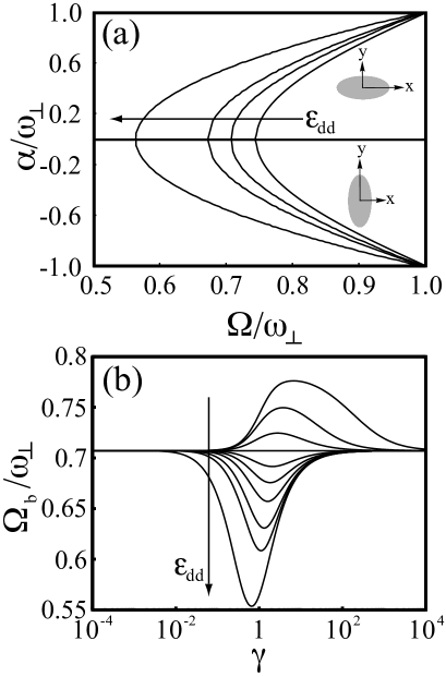
Figure 1: (a) Irrotational velocity field amplitude $\alpha$ of the static condensate solutions as a function of the trap rotation frequency $\Omega$ in a spherically-symmetric trap ($\gamma=1$ and $\epsilon=0$). Various values of $\varepsilon_{dd}$ are presented: $\varepsilon_{dd}=-0.49$, $0$, $0.5$ and $0.99$. Insets illustrate the geometry of the condensate in the $x-y$ plane. (b) The bifurcation frequency $\Omega_{b}$ (the point at which the solutions of $\alpha$ in (a) bifurcate) according to Eq. (30) versus trap ratio $\gamma$. Plotted are the results for $\varepsilon_{dd}=-0.49$, $-0.4$, $-0.2$, $0$, $0.2$, $0.4$, $0.6$, $0.8$, $0.9$ and $0.99$. In (a) and (b) $\varepsilon_{dd}$ increases in the direction of the arrow.

For $\varepsilon_{dd}=0$ we regain the results of Refs. Recati01 ; Sinha01 with a bifurcation point at $\Omega_{b}=\omega_{\perp}/\sqrt{2}$ and, for $\Omega>\Omega_{b}$, non-zero solutions given by $\alpha=\pm\sqrt{2\Omega^{2}-\omega_{\perp}^{2}}/\omega_{\perp}$ Recati01 . The physical significance of the bifurcation frequency has been established for the non-dipolar case and is related to the fact that the system becomes energetically unstable to the spontaneous excitation of quadrupole modes for $\Omega\geq\omega_{\perp}/\sqrt{2}$. In the TF limit, a general surface excitation with angular momentum $\hbar l=\hbar q_{l}R$, where $R$ is the TF radius and $q_{l}$ is the quantized wave number, obeys the classical dispersion relation $\omega_{l}^{2}=(q_{l}/m)\nabla_{R}V$ involving the local harmonic potential $V=m\omega_{\perp}^{2}R^{2}/2$ evaluated at $R$ Pitaevskii&StringariBook . Consequently, for the non-rotating and non-dipolar BEC $\omega_{l}=\sqrt{l}\omega_{\perp}$. Meanwhile, inclusion of the rotational term in the Hamiltonian (10) shifts the mode frequency by $-l\Omega$. Then, in the rotating frame, the frequency of the $l=2$ quadrupole surface excitation becomes $\omega_{2}(\Omega)=\sqrt{2}\omega_{\perp}-2\Omega$ Pitaevskii&StringariBook . The bifurcation frequency thus coincides with the vanishing of the energy of the quadrupolar mode in the rotating frame, and the two additional solutions arise from excitation of the quadrupole mode for $\Omega\geq\omega_{\perp}/\sqrt{2}$.

For the non-dipolar BEC it is noteworthy that $\Omega_{b}$ does not depend on the interactions. This feature arises because the mode frequencies $\omega_{l}$ themselves are independent of $g$. However, in the case of long-range dipolar interactions the potential $\Phi_{dd}$ of Eq. (7) gives non-local contributions, breaking the simple dependence of the force $-\nabla V$ upon $R$ ODell04 . Thus we expect the resonant condition for exciting the quadrupolar mode, i.e. $\Omega_{b}=\omega_{l}/l$ (with $l=2$), to change with $\varepsilon_{dd}$. In Fig. 1(a) we see that this is the case: as dipole interactions are introduced, our solutions change and the bifurcation point, $\Omega_{b}$, moves to lower (higher) frequencies for $\varepsilon_{dd}>0$ ($\varepsilon_{dd}<0$). Note that the parabolic solution still satisfies the hydrodynamic equations providing $-0.5<\varepsilon_{dd}<1$. Outside of this range the parabolic solution may still exist but it is no longer guaranteed to be stable against perturbations.

Density profiles for $\alpha=0$ have zero ellipticity in the $x-y$ plane. By contrast, the $|\alpha|>0$ solutions have an elliptical density profile, even though the trap itself has zero ellipticity. This remarkable feature arises due to a spontaneous breaking of the axial rotational symmetry at the bifurcation point. For $\alpha>0$ the condensate is elongated in $x$ while for $\alpha<0$ it is elongated in $y$, as illustrated in the insets in Fig. 1(a). In the absence of dipolar interactions the $|\alpha|>0$ solutions can be intepreted solely in terms of the effective trapping frequencies ${\tilde{\omega}}_{x}$ and ${\tilde{\omega}}_{y}$ given by Eqs. (18) and (19). The introduction of dipolar interactions considerably complicates this picture, since they also modify the shape of the solutions. Notably, for $\varepsilon_{dd}>0$ the dipolar interactions make the BEC more prolate, i.e., reduce $\kappa_{x}$ and $\kappa_{y}$, while for $\varepsilon_{dd}<0$ they make the BEC more oblate, i.e., increase $\kappa_{x}$ and $\kappa_{y}$.

In Fig. 1(a) we see that as the dipole interactions are increased the bifurcation point $\Omega_{b}$ moves to lower frequencies. The bifurcation point can be calculated analytically as follows. First, we note that for $\alpha=0$ the condensate is cylindrically symmetric and $\kappa_{x}=\kappa_{y}=\kappa$. In this case the aspect ratio $\kappa$ is determined by the transcendental equation Yi00 ; ODell04 ; Eberlein05

$$\left[\left(\frac{\gamma^{2}}{2}+1\right)\frac{f(\kappa)}{1-\kappa^{2}}-1\right]+\frac{\left(\varepsilon_{dd}-1\right)\left(\kappa^{2}-\gamma^{2}\right)}{3\kappa^{2}\varepsilon_{dd}}=0$$

where

$$f(\kappa)=\frac{2+\kappa^{2}\left[4-3\beta_{000}\right]}{2\left(1-\kappa^{2}\right)}$$ (29)

with $\beta_{000}=(1/\sqrt{1-\kappa^{2}})\ln[(1+\sqrt{1-\kappa^{2}})/(1-\sqrt{1-\kappa^{2}})]$ for the prolate case ($\kappa<1$), and $\beta_{000}=(2/\sqrt{\kappa^{2}-1})\arctan[\sqrt{\kappa^{2}-1}]$ for the oblate case ($\kappa>1$). For small $\alpha\rightarrow 0_{+}$, we can calculate the first order corrections to $\kappa_{x}$ and $\kappa_{y}$ with respect to $\kappa$ from Eqs. (24,25). We can then insert these values in Eq. (27) and solve for $\Omega$, noting that in the limit $\alpha\rightarrow 0$ we have $\Omega\rightarrow\Omega_{b}$. Thus, we find

$$\frac{\Omega_{b}}{\omega_{\perp}}=\sqrt{\frac{1}{2}+\frac{3}{4}\kappa^{2}\varepsilon_{dd}\gamma^{2}\frac{\kappa^{2}\beta_{201}-\beta_{101}}{1-\varepsilon_{dd}\left(1-\frac{9}{2}\kappa^{2}\beta_{002}\right)}}.$$ (30)

In Fig. 1(b) we plot $\Omega_{b}$ [Eq. (30)] as a function of $\gamma$ for various values of $\varepsilon_{dd}$. For $\varepsilon_{dd}=0$ we find that the bifurcation point remains unaltered at $\Omega_{b}=\omega_{x}/\sqrt{2}$ as $\gamma=\omega_{z}/\omega_{x}$ is changed Recati01 ; Sinha01 . As $\varepsilon_{dd}$ is increased the value of $\gamma$ for which $\Omega_{b}$ is a minimum changes from a trap shape which is oblate ($\gamma>1$) to prolate ($\gamma<1$). Note that for $\varepsilon_{dd}=0.99$ the minimum bifurcation frequency occurs at $\Omega_{b}\approx 0.55$, which is over a $20\%$ deviation from the non-dipolar value. For more extreme values of $\varepsilon_{dd}$ we can expect $\Omega_{b}$ to deviate even further, although the validity of the inverted parabola TF solution does not necessary hold. For a fixed $\gamma$ we also find that as $\varepsilon_{dd}$ increases the bifurcation frequency decreases monotonically.

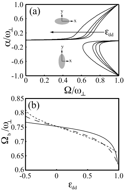
Figure 2: (a) Irrotational velocity field amplitude, $\alpha$, as a function of the trap rotation frequency, $\Omega$, for a trap ratio $\gamma=1$ and ellipticity $\epsilon=0.025$. Various values of $\varepsilon_{dd}$ are presented, $\varepsilon_{dd}=-0.49$, $0$, $0.5$ and $0.99$, with $\varepsilon_{dd}$ increasing in the direction of the arrow. Insets illustrate the geometry of the condensate in the $x-y$ plane. (b) Backbending point $\Omega_{b}$ versus $\varepsilon_{dd}$ for $\epsilon=0.025$ and $\gamma=0.5$ (solid curve), $1.0$ (long dashed curve) and $2.0$ (short dashed curve).

IV.2 Elliptical trapping in the $x-y$ plane: $\epsilon>0$

Consider now the effect of finite ellipticity in the $x-y$ plane ($\epsilon>0$). Rotating elliptical traps have been created experimentally with laser and magnetic fields Madison00 ; Hodby02 . Following the experiment of Madison et al. Madison00 we will employ a weak trap ellipticity of $\epsilon=0.025$. In Fig. 2(a) we have plotted the solutions to Eq. (27) for various values of $\varepsilon_{dd}$ in a $\gamma=1$ trap. As predicted for non-dipolar interactions Recati01 ; Sinha01 the solutions become heavily modified for $\epsilon>0$. There exists an upper branch of $\alpha>0$ solutions which exists over the whole range of $\Omega$, and a lower branch of $\alpha<0$ solutions which back-bends and is double-valued. We term the frequency at which the lower branch back-bends to be the back-bending frequency $\Omega_{b}$. The bifurcation frequency in non-elliptical traps can be regarded as the limiting case of the back-bending frequency, with the differing nonclamenture employed to emphasise the different structure of the solutions at this point. However, for convenience we will employ the same parameter for both, $\Omega_{b}$. No $\alpha=0$ solution exists (for any non-zero $\Omega$). In the absence of dipolar interactions the effect of increasing the trap ellipticity is to increase the back-bending frequency $\Omega_{b}$. Turning on the dipolar interactions, as in the case of $\epsilon=0$, reduces $\Omega_{b}$ for $\varepsilon_{dd}>0$, and increases $\Omega_{b}$ for $\varepsilon_{dd}<0$. This is more clearly seen in Fig. 2(b) where $\Omega_{b}$ is plotted versus $\varepsilon_{dd}$ for various values of the trap ratio $\gamma$. Also, as in the $\epsilon=0$ case, increasing $\varepsilon_{dd}$ decreases both $\kappa_{x}$ and $\kappa_{y}$, i.e. the BEC becomes more prolate.

Importantly, the back-bending of the lower branch can introduce an instability. Consider the BEC to be on the lower branch at some fixed rotation frequency $\Omega$. Now consider decreasing $\varepsilon_{dd}$. The back-bending frequency $\Omega_{b}$ increases and at some point can exceed $\Omega$. In other words, the static solution of the BEC suddenly disappears and the BEC finds itself in an unstable state. We will see in Section VI that this type of instability can also be induced by variations in $\gamma$ and $\epsilon$.

V Dynamical Stability of Stationary Solutions

Although the solutions derived above are static solutions in the rotating frame they are not necessarily stable, and so in this section we analyze their dynamical stability. Consider small perturbations in the BEC density and phase of the form $\rho=\rho_{0}+\delta\rho$ and $S=S_{0}+\delta S$. Then, by linearizing the hydrodynamic equations Eqs. (12, 13), the dynamics of such perturbations can be described as,

$$\frac{\partial}{\partial t}\left[\begin{array}[]{c}\delta S\\ \delta\rho\\ \end{array}\right]=-\left[\begin{array}[]{cc}\underline{v}_{c}\cdot\nabla&g\left(1+\varepsilon_{dd}K\right)/m\\ \nabla\cdot\rho_{0}\nabla&\left[\left(\nabla\cdot\underline{v}\right)+\underline{v}_{c}\cdot\nabla\right]\\ \end{array}\right]\left[\begin{array}[]{c}\delta S\\ \delta\rho\\ \end{array}\right]$$ (37)

where $\underline{v}_{c}=\underline{v}-\underline{\Omega}\times\underline{r}$ and the integral operator $K$ is defined as

$$(K\delta\rho)(\underline{r})=-3\frac{\partial^{2}}{\partial z^{2}}\int\frac{\delta\rho(\underline{r}^{\prime})\ d\underline{r}^{\prime}}{4\pi\left|\underline{r}-\underline{r}^{\prime}\right|}-\delta\rho(\underline{r}).$$ (38)

The integral in the above expression is carried out over the domain where $\rho_{0}>0$, that is, the general ellipsoidal domain with radii $R_{x},R_{y},R_{z}$ of the unperturbed condensate. Extending the integration domain to the region where $\rho_{0}+\delta\rho>0$ adds higher order effects since it is exactly in this domain that $\rho_{0}=\mathcal{O}(\delta\rho)$. To investigate the stability of the BEC we look for eigenfunctions and eigenvalues of the operator (37): dynamical instability arises when one or more eigenvalues $\lambda$ possess a positive real part. The size of the real eigenvalues dictates the rate at which the instability grows. Note that the imaginary eigenvalues of Eq. (37) relate to stable collective modes of the system Castin01 , e.g. sloshing and breathing, and have been analysed elsewhere for dipolar BECs Rick08 . In order to find such eigenfunctions we follow Refs. Bijnen07 ; Sinha01 and consider a polynomial ansatz for the perturbations in the coordinates $x,y$ and $z$, of total degree $N$. All operators in (37), acting on polynomials of degree $N$, result in polynomials of (at most) the same degree, including the operator $K$. This latter fact was known to 19th century astrophysicists who calculated the gravitational potential of a heterogeneous ellipsoid with polynomial density Ferrers ; Dyson . The integral appearing in Eq. (38) is exactly equivalent to such a potential. A more recent paper by Levin and Muratov summarises these results and presents a more manageable expression for the resulting potential LevinMuratov . Hence, using these results the operator $K$ can be evaluated for a general polynomial density perturbation $\delta\rho=x^{p}y^{q}z^{r}$, with $p,q$ and $r$ being non-negative integers and $p+q+r\leq N$. Therefore, the perturbation evolution operator (37) can be rewritten as a scalar matrix operator, acting on vectors of polynomial coefficients, for which finding eigenvectors and eigenvalues is a trivial computational task.

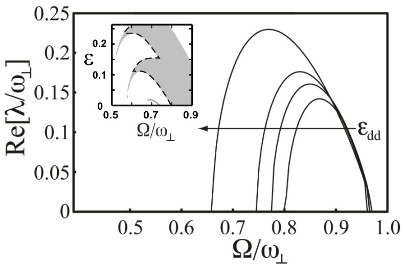
Figure 3: The maximum positive real eigenvalues of Eq. (37) (solid curves) for the upper-branch solutions of $\alpha$ as a function of $\Omega$. We assume $\epsilon=0.025$, $\gamma=1$ and $N=3$, and present various dipolar strengths $\varepsilon_{dd}=-0.49$, $0$, $0.5$ and $0.99$, with $\varepsilon_{dd}$ increasing in the direction of the arrow. The inset shows the full region of dynamical instability in the $\epsilon-\Omega$ plane for $\varepsilon_{dd}=0$. The narrow regions have negligible effect and so we only consider the main instability region (bounded by the dashed line).

Using the above approach we determine the real positive eigenvalues of Eq. (37) and thereby predict the regions of dynamical instability of the static solutions. We focus on the case of an elliptical trap since this is the experimentally relevant case. Recall the general form of the branch diagram for this case, i.e. Fig. 2(a). In the $\alpha<0$ half-plane, the static solutions nearest the $\alpha=0$ axis never become dynamically unstable, except for a small region $\Omega\simeq\omega_{\perp}$, due to a centre-of-mass instability of the condensate Rosenbusch02 . The other lower branch solutions are always dynamically unstable and therefore expected to be irrelevant to experiment. Thus, we only consider dynamical instability for the upper branch solutions, i.e. the branch in the upper half plane (where $\alpha>0$). In Fig. 3 we plot the maximum positive real eigenvalues of the upper branch solutions as a function of $\Omega$ for a fixed ellipticity $\epsilon=0.025$. The maximum polynomial perturbation was set at $N=3$, since for this ellipticity it was found that higher order perturbations did not alter the region of instability, and such modes are therefore not displayed.

For a given $\varepsilon_{dd}$ and $\gamma$ there exists a dynamically unstable region in the $\epsilon-\Omega$ plane. An illustrative example is shown in Fig. 3(inset) for $\varepsilon_{dd}=0$ and $\gamma=1$. The instability region (shaded) consists of a series of crescents Sinha01 . Each crescent corresponds to a single value of the polynomial degree $N$, where higher values of $N$ add extra crescents from above. At the high frequency end these crescents merge to form a main region of instability, characterised by large eigenvalues. At the low frequency end the crescents become vanishingly thin and are characterised by very small eigenvalues which are at least one order of magnitude smaller than in the main instability region Corro07 . As such these regions will only induce instability in the condensate if they are traversed very slowly. This was confirmed by numerical simulations in Ref. Corro07 where it was shown that the narrow instability regions have negligible effect when ramping $\Omega$ at rates greater than $d\Omega/dt=2\times 10^{-4}\omega_{\perp}^{2}$. It is unlikely that an experiment could be sufficiently long-lived for these narrow instability regions to play a role. For this reason we will subsequently ignore the narrow regions of instability and define our instability region to be the main region, as bounded by the dashed line in Fig. 3(inset). For the experimentally relevant trap ellipticities $\epsilon\raisebox{-2.58334pt}{$\,\stackrel{{\scriptstyle\raisebox{-0.60275pt}{$\textstyle<$}}}{{\sim}}\,$}0.1$ the unstable region is defined solely by the $N=3$ perturbations.

We define the lower bound of the instability region to be $\Omega_{i}$ (this corresponds to the dashed line in the inset). This is the key parameter to characterise the dynamical instability. As $\varepsilon_{dd}$ is increased $\Omega_{i}$ decreases and, accordingly, the unstable range of $\Omega$ widens. Note that the upper bound of the instability region is defined by the endpoint of the upper branch at $\Omega\simeq\omega_{\perp}$.

VI Routes to instability and vortex lattice formation

VI.1 Procedures to induce instability

For a non-dipolar BEC the static solutions and their stability in the rotating frame depend only on rotation frequency $\Omega$ and trap ellipticity $\epsilon$. Adiabatic changes in $\epsilon$ and $\Omega$ can be employed to evolve the condensate through the static solutions and reach a point of instability. Indeed, this has been realized both experimentally Madison00 ; Hodby02 and numerically Lundh03 ; Parker06 , with excellent agreement to the hydrodynamic predictions. For the case of a dipolar BEC we have shown in Sections IV and V that the static solutions and their instability depend additionally on the trap ratio $\gamma$ and the interaction parameter $\varepsilon_{dd}$. Since all of these parameters can be experimentally tuned in time, one can realistically consider each parameter as a distinct route to traverse the parameter space of solutions and induce instability in the system.

Examples of these routes are presented in Fig. 4. Specifically, Fig. 4 shows the static solutions $\alpha$ of Eq. (27) as a function of $\Omega$ [Fig. 4(a)], $\epsilon$ [Fig. 4(b)], $\varepsilon_{dd}$ [Fig. 4(c)] and $\gamma$ [Fig. 4(d)]. In each case the remaining three parameters are fixed at $\epsilon=0.025$, $\gamma=1$, $\Omega=0.7\omega_{\perp}$, and $\varepsilon_{dd}=0.99$. Dynamically unstable solutions are indicated with red circles. Grey arrows mark routes towards instability (the point of onset of instability being marked by an asterisk), where the free parameter $\Omega$, $\epsilon$, $\varepsilon_{dd}$, or $\gamma$ is varied adiabatically until either a dynamical instability is reached, or the solution branch backbends and so ceases to exist. For solutions with $\alpha>0$, the instability is always due to the system becoming dynamically unstable (dashed arrows), whereas for $\alpha<0$ the instability is always due to the solution branch backbending on itself (solid arrows) and so ceasing to exist. Numerical studies Parker06 indicate that these two types of instability involve different dynamics and possibly have distinct experimental signatures.

Below we describe adiabatic variation of each parameter in more general detail, beginning with the established routes towards instability in which (i) $\Omega$ and (ii) $\epsilon$ are varied, and then novel routes based on adiabatic changes in (iii) $\varepsilon_{dd}$ and (iv) $\gamma$. In each case it is crucial to consider the behaviour of the points of instability, namely the back-bending point $\Omega_{b}$ and the onset of dynamical instability of the upper branch $\Omega_{i}$.

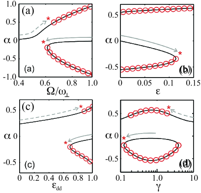
Figure 4: Stationary states in the rotating trap characterised by the velocity field amplitude $\alpha$, determined from Eq. (27). Dynamically unstable solutions are marked with red circles. In each of the figures the trap rotation frequency $\Omega$ (a), trap ellipticity $\epsilon$ (b), dipolar interaction strength $\varepsilon_{dd}$ (c) and axial trapping strength $\gamma$ (d) are varied adiabatically, whilst the remaining parameters remain fixed at $\Omega=0.7\omega_{\perp}$, $\epsilon=0.025$, $\varepsilon_{dd}=0.99$, and $\gamma=1$. The adiabatic pathways to instability (onset marked by red asterisk) are schematically shown by the dashed and solid arrows. Dashed arrows indicate a route towards dynamical instability, whereas solid arrows indicate an instability due to disappearance of the stationary state.

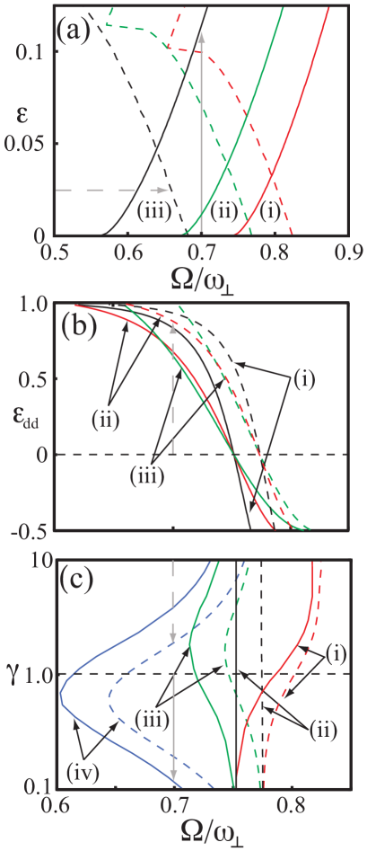
Figure 5: (a) Phase diagram of $\epsilon$ versus $\Omega_{b}$ (solid curves) and $\Omega_{i}$ (dashed curves) for $\gamma=1$ and (i) $\varepsilon_{dd}=-0.49$, (ii) $0.5$ and (iii) $0.99$. (b) Phase diagram of $\varepsilon_{dd}$ versus $\Omega_{b}$ (solid curves) and $\Omega_{i}$ (dashed curves) for $\epsilon=0.025$ and (i) $\gamma=0.5$, (ii) $1$ and (iii) $2$. (c) Phase diagram of $\gamma$ versus $\Omega_{b}$ (solid curves) and $\Omega_{i}$ (dashed curves) for $\epsilon=0.025$ and (i) $\varepsilon_{dd}=-0.49$, (ii) $0$, (iii) $0.5$ and (iv) $0.99$. In each case the solid (dashed) arrows depict the routes to instability shown in Fig. 4.

i) Adiabatic introduction of $\Omega$: The relevant parameter space of $\epsilon$ and $\Omega$ is presented in Fig. 5(a), with the instability frequencies $\Omega_{b}(\epsilon)$ (solid curves) and $\Omega_{i}(\epsilon)$ (dashed curves) indicated. For a BEC initially confined to a non-rotating trap with finite ellipticity $\epsilon$, as the rotation frequency $\Omega$ is increased adiabatically the BEC follows the upper branch solution [Fig. 4(a) (dashed arrow)]. This particular route traces out a horizontal path in Fig. 5(a) until it reaches $\Omega_{i}(\epsilon)$, where the stationary solution becomes dynamically unstable. For the specific parameters of Fig. 4(a) the system becomes unstable at $\Omega=\Omega_{i}(\epsilon)\approx 0.65\omega_{\perp}$. More generally, Fig. 5(a) shows that as $\varepsilon_{dd}$ is increased, $\Omega_{i}(\epsilon)$ is decreased and as such instabilities in the stationary solutions will occur at lower rotation frequencies. At $\epsilon\simeq 0.1$, the curve for $\Omega_{i}$ displays a sharp kink, arising from the shape of the dynamically unstable region, as shown in Fig. 3(inset).

ii) Adiabatic introduction of $\epsilon$: Here we begin with a cylindrically symmetric ($\epsilon=0$) trap, rotating at a fixed frequency $\Omega$. The trap ellipticity $\epsilon$ is then increased adiabatically and in the phase diagram of Fig. 5(a) the BEC traces out a vertical path starting at $\epsilon=0$. The ensuing dynamics depend on the trap rotation speed relative to $\Omega_{b}(\epsilon=0)$:

(a) For $\Omega<\Omega_{b}(\epsilon=0)$ the condensate follows the upper branch of the static solutions shown in Fig. 4(a). This branch moves progressively to larger $\alpha$. For $\Omega<\Omega_{i}(\epsilon)$ the BEC remains stable but as $\epsilon$ is increased further the condensate eventually becomes dynamically unstable. Figure 5(a) shows that as $\varepsilon_{dd}$ is increased $\Omega_{i}(\epsilon)$ is decreased and as such the dynamical instability of the stationary solutions occurs at a lower trap ellipticity.

(b) For $\Omega>\Omega_{b}(\epsilon=0)$ the condensate accesses the lower branch solutions nearest the $\alpha=0$ axis. These solutions are always dynamically stable and the criteria for instability is instead determined by whether the solution exists. As $\epsilon$ is increased the back-bending frequency $\Omega_{b}(\epsilon)$ increases. Therefore, when $\epsilon$ exceeds some critical value the lower branch solutions disappear for the chosen value of rotation frequency $\Omega$. This occurs when $\Omega<\Omega_{b}(\epsilon)$. Figure 5(a) shows that as $\varepsilon_{dd}$ is increased $\Omega_{b}(\epsilon)$ is decreased and as such instabilities in the system will occur at a higher trap ellipticity. At this point the parabolic condensate density profile no longer represents a stable solution. The particular route indicated in Fig. 4(b) is included in Fig. 5(a) as a vertical, solid grey arrow.

iii) Adiabatic change of $\varepsilon_{dd}$: The relevant parameter space of $\varepsilon_{dd}$ and $\Omega$ is shown in Fig. 5(b) for several different trap ratios. Consider that we begin from an initial BEC in a trap with finite ellipticity $\epsilon=0.025$ and rotation frequency $\Omega$. (This can be achieved, for example, by increasing $\epsilon$ from zero at fixed $\Omega$.) Then, by changing $\varepsilon_{dd}$ adiabatically an instability can be induced in two ways:

(a) For $\Omega<\Omega_{b}(\varepsilon_{dd})$ the condensate follows the upper branch solutions until they become unstable. This route to instability in shown in Fig. 4(c) by the dashed arrow, with the corresponding path in Fig. 5(b) shown by the vertical dashed arrow. Thus for $\Omega<\Omega_{i}(\varepsilon_{dd})$ the motion remains stable. However, for $\Omega>\Omega_{i}(\varepsilon_{dd})$ the upper branch becomes dynamically unstable. In Fig. 5(b) $\Omega_{i}(\varepsilon_{dd})$ (dashed curves) is plotted for different trap ratios. As can be seen, the stable region of the upper branch becomes smaller as $\varepsilon_{dd}$ is increased.

(b) For $\Omega>\Omega_{b}(\varepsilon_{dd})$ the condensate follows the lower branch solutions nearest the $\alpha=0$ axis. These solutions are always stable and hence an instability can only be induced when this solution no longer exists, i.e. $\Omega<\Omega_{b}(\varepsilon_{dd})$. Figure 5(b) shows $\Omega_{b}(\varepsilon_{dd})$ (solid curves) for various trap aspect ratios. As can be seen the back-bending frequency $\Omega_{b}$ decreases as $\varepsilon_{dd}$ is increased. Thus if $\varepsilon_{dd}$ is increased the system will remain stable. However if $\varepsilon_{dd}$ is decreased then the system will become unstable when $\Omega=\Omega_{b}(\varepsilon_{dd})$.

iv) Adiabatic change of $\gamma$: Figure 5(c) shows the parameter space of $\gamma$ and $\Omega$. Consider, again, an initial stable condensate with finite trap rotation frequency $\Omega$ and ellipticity $\epsilon=0.025$. Then through adiabatic changes in $\gamma$ the condensate can traverse the parameter space and, depending on the initial conditions, the instability can arise in two ways:

(a) For $\Omega<\Omega_{b}(\gamma)$ the condensate exists on the upper branch. It is then relevant to consider the onset of dynamical instability $\Omega_{i}(\gamma)$ (dashed curves in Fig. 5(c)). Providing $\Omega<\Omega_{i}(\gamma)$ the solution remains dynamically stable. However, once $\Omega>\Omega_{i}(\gamma)$ the upper branch solutions become unstable.

(b) For $\Omega>\Omega_{b}(\gamma)$ the condensate exists on the lower branch nearest the $\alpha=0$ axis. These solutions are always dynamically stable and instability can only occur when the motion of the back-bending point causes the solution to disappear. This occurs when $\Omega<\Omega_{b}(\gamma)$, with $\Omega_{b}(\gamma)$ shown in Fig. 5(c) by solid curves for various dipolar interaction strengths.

These two paths to instability are shown in Fig. 4(d) and are also indicated in Fig. 5(c) as vertical grey arrows, where the dashed (solid) arrow corresponds to the $\alpha>0$ ($\alpha<0$) path.

VI.2 Is the final state of the system a vortex lattice?

Having revealed the points at which a rotating dipolar condensate becomes unstable we will now address the question of whether this instability leads to a vortex lattice. First, let us review the situation for a non-dipolar BEC. The presence of vortices in the system becomes energetically favorable when the rotation frequency exceeds a critical frequency $\Omega_{v}$. Working in the TF limit, with the background density taking the parabolic form (9), $\Omega_{v}$ can be approximated as lundh97 ,

$$\Omega_{v}=\frac{5}{2}\frac{\hbar}{mR^{2}}\ln\frac{0.67R}{\xi_{s}}.$$ (39)

Here the condensate is assumed to be circularly symmetric with radius $R$, and $\xi_{s}=\hbar/\sqrt{2m\rho_{0}g}$ is the healing length that characterises the size of the vortex core. For typical condensate parameters $\Omega_{v}\sim 0.4\omega_{\perp}$. It is observed experimentally, however, that vortex lattice formation occurs at considerably higher frequencies, typically $\Omega\sim 0.7\omega_{\perp}$. This difference arises because above $\Omega_{v}$ the vortex-free solutions remain remarkably stable. It is only once a hydrodynamic instability occurs (which occurs in the locality of $\Omega\approx 0.7\omega_{\perp}$) that the condensate has a mechanism to deviate from the vortex-free solution and relax into a vortex lattice. Another way of visualising this is as follows. Above $\Omega_{v}$ the vortex-free condensate resides in some local energy minimum, while the global minimum represents a vortex or vortex lattice state. Since the vortex is a topological defect, there typically exists a considerable energy barrier for a vortex to enter the system. However, the hydrodynamic instabilities offer a route to navigate the BEC out of the vortex-free local energy minimum towards the vortex lattice state.

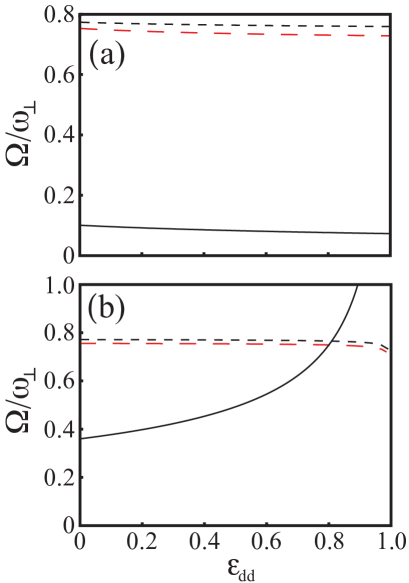
Figure 6: The relation between the instability frequencies, $\Omega_{b}$ (long dashed red curve) and $\Omega_{i}$ (short dashed curve), and the critical rotation frequency for vorticity $\Omega_{v}$ (solid curve) for (a) an oblate trap $\gamma=10$ and (b) a prolate trap $\gamma=0.1$. The instability frequencies are based on a trap with ellipticity $\epsilon=0.025$ while $\Omega_{v}$ is obtained from Eq. (39) under the assumption of a ⁵²Cr BEC with $150,000$ atoms and scattering length $a_{s}=5.1$nm in a circularly symmetric trap with $\omega_{\perp}=2\pi\times 200$Hz.

Note that vortex lattice formation occurs via non-trivial dynamics. The initial hydrodynamic instability in the vortex-free state that we have discussed in this paper is only the first step Parker06 . For example, if the condensate is on the upper branch of hydrodynamic solutions (e.g. under adiabatic introduction of $\Omega$) and undergoes a dynamical instability, this leads to the exponential growth of surface ripples in the condensate Parker06 ; Madison00 . Alternatively, if the condensate is on the lower branch and the static solutions disappear (e.g. following the introduction of $\epsilon$) the condensate undergoes large and dramatic shape oscillations. In both cases the destabilisation of the vortex-free condensate leads to the nucleation of vortices into the system. A transient turbulent state of vortices and density perturbations then forms, which subsequently relaxes into a vortex lattice configuration Parker06 ; Parker05 .

In the presence of dipolar interactions, however, the critical frequency for a vortex depends crucially on the trap geometry $\gamma$ and the strength of the dipolar interactions $\varepsilon_{dd}$. Following reference ODell07 we will make a simple and approximated extension of Eq. (39) to a dipolar BEC. We will consider a circularly-symmetric dipolar condensate with radius $R=R_{x}=R_{y}$ that satisfies Eqs. (24)-(26), and insert this into Eq. (39) for the condensate radius. This method still assumes that the size of the vortex is characterised by the s-wave healing length $\xi_{s}$. Although one does expect the dipolar interactions to modify the size of the vortex core, it should be noted that Eq. (39) only has logarithmic accuracy and is relatively insensitive to the choice of vortex core length scale. The dominant effect of the dipolar interactions in Eq. (39) comes from the radial size and is accounted for. Note also that this expression is for a circularly symmetric system while we are largely concerned with elliptical traps. However we will employ a very weak ellipticity $\epsilon=0.025$ for which we expect the correction to the critical frequency to be correspondingly small.

As an example, we take the parameter space of rotation frequency $\Omega$ and dipolar interactions $\varepsilon_{dd}$. We first consider the behavior in a quite oblate trap with $\gamma=10$. In Fig. 6(a) we plot the instability frequencies $\Omega_{i}$ and $\Omega_{b}$ for this system as a function of the dipolar interactions $\varepsilon_{dd}$. Depending on the specifics of how this parameter space is traversed, either by adiabatic changes in $\Omega$ (vertical path) or $\varepsilon_{dd}$ (horizontal path), the condensate will become unstable when it reaches one of the instability lines (short and long dashed lines). These points of instability decrease weakly with dipolar interactions and have the approximate value $\Omega_{i}\approx\Omega_{b}\approx 0.75\omega_{\perp}$. On the same plot we present the critical rotation frequency $\Omega_{v}$ according to Eq. (39). In order to calculate this we have assumed a BEC of 150,000 ⁵²Cr atoms confined within a trap with $\omega_{\perp}=2\pi\times 200$Hz. In this oblate system we see that the dipolar interactions lead to a decrease in $\Omega_{v}$, as noted in ODell07 . This dependence is very weak at this value of $\gamma$, and throughout the range of $\varepsilon_{dd}$ presented it maintains the approximate value $\Omega_{v}\approx 0.1\omega_{\perp}$. Importantly these results show that when the condensate becomes unstable a vortex/vortex lattice state is energetically favored. As such, we expect that in an oblate dipolar BEC a vortex lattice will ultimately form when these instabilities are reached.

In Fig. 6(b), we make a similar plot but for a prolate trap with $\gamma=0.1$. The instability frequencies show a somewhat similar behaviour to the oblate case. However, $\Omega_{v}$ is drastically different, increasing significantly with $\varepsilon_{dd}$. We find that this qualitative behaviour occurs consistently in prolate systems, as noted in ODell07 . This introduces two regimes depending on the dipolar interactions. For $\varepsilon_{dd}\raisebox{-2.58334pt}{$\,\stackrel{{\scriptstyle\raisebox{-0.60275pt}{$\textstyle<$}}}{{\sim}}\,$}0.8$, $\Omega_{i,b}>\Omega_{v}$, and so we expect a vortex/vortex lattice state to form following the instability. However, for $\varepsilon_{dd}\raisebox{-2.58334pt}{$\,\stackrel{{\scriptstyle\raisebox{-0.60275pt}{$\textstyle>$}}}{{\sim}}\,$}0.8$ we find an intriguing new regime in which $\Omega_{i,b}<\Omega_{v}$. In other words, while the instability in the vortex-free parabolic density profile still occurs, a vortex state is not energetically favorable. The final state of the system is therefore not clear. Given that a prolate dipolar BEC is dominated by attractive interactions (since the dipoles lie predominantly in an attractive end-to-end configuration) one might expect similar behavior to the case of conventional BECs with attractive interactions ($g<0$) where the formation of a vortex lattice can also be energetically unfavorable. Suggestions for final state of the condensate in this case include centre-of-mass motion and collective oscillations, such as quadrupole modes or higher angular momentum-carrying shape excitations Wilkin98 ; Mottelson99 ; Pethick00 . However the nature of the true final state in this case is beyond the scope of this work and warrants further investigation.

VII Conclusions

By calculating the static hydrodynamic solutions of a rotating dipolar BEC and studying their stability, we have predicted the regimes of stable and unstable motion. In general we find that the backbending or bifurcation frequency $\Omega_{b}$ decreases with increasing dipolar interactions. In addition, the onset of dynamical instability in the upper branch solutions, $\Omega_{i}$, decreases with increasing dipolar interactions. Furthermore these frequencies depend on the aspect ratio of the trap.

By utilising the novel features of dipolar condensates we detail several routes to traverse the parameter space of static solutions and reach a point of instability. This can be achieved through adiabatic changes in trap rotation frequency $\Omega$, trap ellipticity $\epsilon$, dipolar interactions $\varepsilon_{dd}$ and trap aspect ratio $\gamma$, all of which are experimentally tunable quantities. While the former two methods have been employed for non-dipolar BECs, the latter two methods are unique to dipolar BECs. In an experiment the latter instabilities would therefore demonstrate the special role played by dipolar interactions. Furthermore, unlike for conventional BECs with repulsive interactions, the formation of a vortex lattice following a hydrodynamic instability is not always favored and depends sensitively on the shape of the system. For a prolate BEC with strong dipolar interactions there exists a regime in which the rotating spheroidal parabolic Thomas-Fermi density profile is unstable and yet it is energetically unfavorable to form a lattice. Other outcomes may then develop, such as a centre-of-mass motion of the system or collective modes with angular momentum. However, for oblate dipolar condensates, as well as prolate condensates with weak dipolar interactions, the presence of vortices is energetically favored at the point of instability and we expect the instability to lead to the formation of a vortex lattice.

We acknowledge financial support from the Australian Research Council (AMM), the Government of Canada (NGP) and the Natural Sciences and Engineering Research Council of Canada (DHJOD).

References

- (1) A. Griesmaier,J. Werner, S. Hensler, J. Stuhler and T. Pfau, Phys. Rev. Lett. 94, 160401 (2005).
- (2) T. Lahaye, T. Koch, B. Frohlich, M. Fattori, J. Metz, A. Griesmaier, S. Giovanazzi and T. Pfau, Nature (London) 448, 672 (2007).
- (3) T. Koch, T. Lahaye, J. Metz, B. Frohlich, A. Griesmaier and T. Pfau, Nat. Phys. 4, 218 (2008).
- (4) L. Santos, G.V. Shlyapnikov, P. Zoller, and M. Lewenstein, Phys. Rev. Lett. 85, 1791 (2000).
- (5) S. Yi and L. You, Phys. Rev. A 63, 053607 (2001).
- (6) C. J. Pethick and H. Smith, Bose-Einstein Condensation in Dilute Gases (Cambridge University Press, 2002).
- (7) L. Pitaevskii and S. Stringari, Bose-Einstein Condensation (Oxford, 2003), p183.
- (8) P. Nozieres and D. Pines, Theory Of Quantum Liquids (Westview, New York, 1999).
- (9) S. Stringari, Phys. Rev. Lett. 77, 2360 (1996).
- (10) N.G. Parker and D. H. J. O’Dell, Phys. Rev. A 78, 041601(R) (2008).
- (11) D. H. J. O’Dell, S. Giovanazzi and C. Eberlein, Phys. Rev. Lett. 92, 250401 (2004).
- (12) C. Eberlein, S. Giovanazzi and D.H.J. O’Dell, Phys. Rev. A 71, 033618 (2005).
- (13) K. W. Madison, F. Chevy, W. Wohlleben and J. Dalibard, Phys. Rev. Lett. 84, 806, (2000); K. W. Madison, F. Chevy, V. Bretin and J. Dalibard, ibid. 86 4443 (2001).
- (14) E. Hodby et al., Phys. Rev. Lett. 88, 010405 (2002).
- (15) A. Recati, F. Zambelli and S. Stringari, Phys. Rev. Lett. 86, 377 (2001).
- (16) S. Sinha and Y. Castin, Phys. Rev. Lett. 87, 190402 (2001).
- (17) E. Lundh, J.-P. Martikainen and K.-A. Suominen, Phys. Rev. A 67, 063604 (2003).
- (18) N. G. Parker, R. M. W. van Bijnen and A. M. Martin, Phys. Rev. A 73, 061603(R) (2006).
- (19) I. Corro, N. G. Parker and A. M. Martin, J. Phys. B 40, 3615 (2007).
- (20) S. Yi and H. Pu, Phys. Rev. A 73, 061602(R) (2006).
- (21) D. H. J. O’Dell and C. Eberlein, Phys. Rev. A 75, 013604 (2007).
- (22) R. M. Wilson, S. Ronen, J. L. Bohn, and H. Pu, Phys. Rev. Lett. 100, 245302 (2008).
- (23) N. R. Cooper, E. H. Rezayi and S. H. Simon, Phys. Rev. Lett. 95 200402 (2005).
- (24) J. Zhang and H. Zhai, Phys. Rev. Lett. 95, 200403 (2005).
- (25) S. Komineas and N. R. Cooper, Phys. Rev. A 75, 023623 (2007).
- (26) R. M. W. van Bijnen, D. H. J. O’Dell, N. G. Parker and A. M. Martin, Phys. Rev. Lett. 98, 150401 (2007).
- (27) A. M. Martin, N. G. Parker, R. M. W. van Bijnen, A. Dow and D. H. J. O’Dell, Las. Phys. 18, 322 (2008).
- (28) K. Góral, K. Rza̧żewski, and T. Pfau, Phys. Rev. A 61, 051601 (2000).
- (29) S. Yi and L. You, Phys. Rev. A 61, 041604 (2000).
- (30) M. Marinescu and L. You, Phys. Rev. Lett. 81, 4596 (1998).
- (31) S. Giovanazzi, A. Gorlitz and T. Pfau, Phys. Rev. Lett. 89, 130401 (2002).
- (32) N. G. Parker, C. Ticknor, A. M. Martin and D. H. O’Dell, Phys. Rev. A 79, 013617 (2009).
- (33) A. J. Leggett, Quantum Liquids: Bose-Condensation and Cooper Pairing in Condensed Matter Systems (Oxford University Press, 2006).
- (34) A. J. Leggett, in Bose-Einstein Condensation: From Atomic Physics to Quantum Fluids, Proceedings of the Thirteenth Physics Summer School, edited by C. M. Savage and M. P. Das, (World Scientific, 2001), p. 1-42.
- (35) L. D. Landau and E. M. Lifshitz, Course of Theoretical Physics: Mechanics (Butterworth-Heinemann, third edition, 1982)
- (36) L. S. Gradshteyn and I. M. Ryzhik, eds., Table of Integrals, Series, and Products (Academic Press, San Diego, 2000), sixth ed.
- (37) M. Abramowitz and I. Stegun, eds., Handbook of Mathematical Functions (Dover, New York, 1974).
- (38) Y. Castin, in Coherent Matter Waves, Lecture Notes of Les Houches Summer School, edited by R. Kaiser, C. Westbrook and F. David (Springer-Verlag, 2001), p. 1-136.
- (39) R. M. W. van Bijnen, N. G. Parker, A. M. Martin and D. H. J. O’Dell, preprint (2008).
- (40) N. M. Ferrers, Quart. J. Pure and Appl. Math 14, 1 (1877).
- (41) F. W. Dyson, Quart. J. Pure and Appl. Math, 25, 259 (1891).
- (42) M. L. Levin and R. Z. Muratov, Astrophys. J. 166, 441 (1971).
- (43) P. Rosenbusch, D.S. Petrov, S. Sinha, F. Chevy, V. Bretin, Y. Castin, G. Shlyapnikov, and J. Dalibard, Phys. Rev. Lett. 88, 250403, (2002)
- (44) E. Lundh, C.J. Pethick and H. Smith, Phys. Rev. A 55, 2126 (1997).
- (45) N. K. Wilkin, J.M.F. Gunn and R.A. Smith, Phys. Rev. Lett. 80, 2265 (1998).
- (46) B. Mottelson, Phys. Rev. Lett. 83, 2695 (2000).
- (47) C. J. Pethick and L. Pitaevskii, Phys. Rev. A 62, 033609 (2000).
- (48) N. G. Parker and C. S. Adams, Phys. Rev. Lett. 95, 145301 (2005); J. Phys. B 39, 43 (2006).
- (49) E. Lundh, C. J. Pethink and H. Smith, Phys. Rev. A 55, 2126 (1997).