Numerical analysis of nonlinear eigenvalue problems

Abstract

We provide a priori error estimates for variational approximations of the ground state energy, eigenvalue and eigenvector of nonlinear elliptic eigenvalue problems of the form $-\mbox{div}(A\nabla u)+Vu+f(u^{2})u=\lambda u$, $\|u\|_{L^{2}}=1$. We focus in particular on the Fourier spectral approximation (for periodic problems) and on the $\mathbb{P}_{1}$ and $\mathbb{P}_{2}$ finite-element discretizations. Denoting by $(u_{\delta},\lambda_{\delta})$ a variational approximation of the ground state eigenpair $(u,\lambda)$, we are interested in the convergence rates of $\|u_{\delta}-u\|_{H^{1}}$, $\|u_{\delta}-u\|_{L^{2}}$, $|\lambda_{\delta}-\lambda|$, and the ground state energy, when the discretization parameter $\delta$ goes to zero. We prove in particular that if $A$, $V$ and $f$ satisfy certain conditions, $|\lambda_{\delta}-\lambda|$ goes to zero as $\|u_{\delta}-u\|_{H^{1}}^{2}+\|u_{\delta}-u\|_{L^{2}}$. We also show that under more restrictive assumptions on $A$, $V$ and $f$, $|\lambda_{\delta}-\lambda|$ converges to zero as $\|u_{\delta}-u\|_{H^{1}}^{2}$, thus recovering a standard result for linear elliptic eigenvalue problems. For the latter analysis, we make use of estimates of the error $u_{\delta}-u$ in negative Sobolev norms.

1 Introduction

Many mathematical models in science and engineering give rise to nonlinear eigenvalue problems. Let us mention for instance the calculation of the vibration modes of a mechanical structure in the framework of nonlinear elasticity, the Gross-Pitaevskii equation describing the steady states of Bose-Einstein condensates [9], or the Hartree-Fock and Kohn-Sham equations used to calculate ground state electronic structures of molecular systems in quantum chemistry and materials science (see [3] for a mathematical introduction).

The numerical analysis of linear eigenvalue problems has been thoroughly studied in the past decades (see e.g. [1]). On the other hand, only a few results on nonlinear eigenvalue problems have been published so far [13, 14].

In this article, we focus on a particular class of nonlinear eigenvalue problems arising in the study of variational models of the form

$$I=\inf\left\{E(v),\;v\in X,\;\int_{\Omega}v^{2}=1\right\}$$ (1)

where

$$\left|\begin{array}[]{l}\Omega\mbox{ is a regular bounded domain or a rectangular brick of $\mathbb{R}^{d}$ and }X=H^{1}_{0}(\Omega)\\ \mbox{or}\\ \Omega\mbox{ is the unit cell of a periodic lattice ${\cal R}$ of $\mathbb{R}^{d}$ and }X=H^{1}_{\#}(\Omega)\end{array}\right.$$

with $d=1$, $2$ or $3$, and where the energy functional $E$ is of the form

$$E(v)=\frac{1}{2}a(v,v)+\frac{1}{2}\int_{\Omega}F(v^{2}(x))\,dx$$

with

$$a(u,v)=\int_{\Omega}(A\nabla u)\cdot\nabla v+\int_{\Omega}Vuv.$$

Recall that if $\Omega$ is the unit cell of a periodic lattice ${\cal R}$ of $\mathbb{R}^{d}$, then for all $s\in\mathbb{R}$ and $k\in\mathbb{N}$,

$$H^{s}_{\#}(\Omega) = \left\{v|_{\Omega},\;v\in H^{s}_{\rm loc}(\mathbb{R}^{d})\;|\;v\;{\cal R}\mbox{-periodic}\right\},$$

$$C^{k}_{\#}(\Omega) = \left\{v|_{\Omega},\;v\in C^{k}(\mathbb{R}^{d})\;|\;v\;{\cal R}\mbox{-periodic}\right\}.$$

We assume in addition that

$$\bullet A\in(L^{\infty}({\Omega}))^{d\times d}\mbox{ and }A(x)\mbox{ is symmetric for almost all }x\in\Omega$$ (3)

$$\exists\alpha>0\mbox{ s.t. }\xi^{T}A(x)\xi\geq\alpha|\xi|^{2}\mbox{ for all }\xi\in\mathbb{R}^{d}\mbox{ and almost all }x\in\Omega$$

$$\bullet V\in L^{p}(\Omega)\mbox{ for some }p>\max(1,d/2)$$ (4)

$$\bullet F\in C^{1}([0,+\infty),\mathbb{R})\cap C^{2}((0,\infty),\mathbb{R})\mbox{ and }F^{\prime\prime}>0\mbox{ on }(0,+\infty)$$ (7)

$$\exists 0\leq q<2,\;\exists C\in\mathbb{R}_{+}\mbox{ s.t. }\forall t\geq 0,\;|F^{\prime}(t)|\leq C(1+t^{q})$$

$$F^{\prime\prime}(t)t\mbox{ remains bounded in the vicinity of }0.$$

To establish some of our results, we will also need to make the additional assumption that there exists $1<r\leq 2$ and $0\leq s\leq 5-r$ such that

$$\forall R>0,\;\exists C_{R}\in\mathbb{R}_{+}\mbox{ s.t. }\forall 0<t_{1}\leq R,\;\forall t_{2}\in\mathbb{R},\;$$

$$\quad\left|F^{\prime}(t_{2}^{2})t_{2}-F^{\prime}(t_{1}^{2})t_{2}-2F^{\prime\prime}(t_{1}^{2})t_{1}^{2}(t_{2}-t_{1})\right|\leq C_{R}\left(1+|t_{2}|^{s}\right)|t_{2}-t_{1}|^{r}.$$ (8)

Note that for all $1<m<3$ and all $c>0$, the function $F(t)=ct^{m}$ satisfies (7)-(7) and (8), for some $1<r\leq 2$. It satisfies (8) with $r=2$ if $3/2\leq m<3$. This allows us to handle the Thomas-Fermi kinetic energy functional ($m=\frac{5}{3}$) as well as the repulsive interaction in Bose-Einstein condensates ($m=2$).

Remark 1

Assumption (7) is sharp for $d=3$, but is useless for $d=1$ and can be replaced with the weaker assumption that there exist $q<\infty$ and $C\in\mathbb{R}_{+}$ such that $|F^{\prime}(t)|\leq C(1+t^{q})$ for all $t\in\mathbb{R}_{+}$, for $d=2$. Likewise, the condition $0\leq s\leq 5-r$ in assumption (8) is sharp for $d=3$ but can be replaced with $0\leq s<\infty$ if $d=1$ or $d=2$.

In order to simplify the notation, we denote by $f(t)=F^{\prime}(t)$.

Making the change of variable $\rho=v^{2}$ and noticing that $a(|v|,|v|)=a(v,v)$ for all $v\in X$, it is easy to check that

$$I=\inf\left\{{\cal E}(\rho),\;\rho\geq 0,\;\sqrt{\rho}\in X,\;\int_{\Omega}\rho=1\right\},$$ (9)

where

$${\cal E}(\rho)=\frac{1}{2}a(\sqrt{\rho},\sqrt{\rho})+\frac{1}{2}\int_{\Omega}F(\rho).$$

We will see that under assumptions (3)-(7), (9) has a unique solution $\rho_{0}$ and (1) has exactly two solutions: $u=\sqrt{\rho_{0}}$ and $-u$. Moreover, $E$ is $C^{1}$ on $X$ and for all $v\in X$, $E^{\prime}(v)=A_{v}v$ where

$$A_{v}=-\mbox{div}(A\nabla\cdot)+V+f(v^{2}).$$

Note that $A_{v}$ defines a self-adjoint operator on $L^{2}(\Omega)$, with form domain $X$. The function $u$ therefore is solution to the Euler equation

$$\forall v\in X,\quad\langle A_{u}u-\lambda u,v\rangle_{X^{\prime},X}=0$$ (10)

for some $\lambda\in\mathbb{R}$ (the Lagrange multiplier of the constraint $\|u\|_{L^{2}}^{2}=1$) and equation (10), complemented with the constraint $\|u\|_{L^{2}}=1$, takes the form of the nonlinear eigenvalue problem

$$\left\{\begin{array}[]{l}A_{u}u=\lambda u\\ \|u\|_{L^{2}}=1.\end{array}\right.$$ (11)

In addition, $u\in C^{0}(\overline{\Omega})$, $u>0$ in $\Omega$ and $\lambda$ is the ground state eigenvalue of the linear operator $A_{u}$. An important result is that $\lambda$ is a simple eigenvalue of $A_{u}$. It is interesting to note that $\lambda$ is also the ground state eigenvalue of the nonlinear eigenvalue problem

$$\left\{\begin{array}[]{l}\mbox{search }(\mu,v)\in\mathbb{R}\times X\mbox{ such that}\\ A_{v}v=\mu v\\ \|v\|_{L^{2}}=1,\end{array}\right.$$ (12)

in the following sense: if $(\mu,v)$ is solution to (12) then either $\mu>\lambda$ or $\mu=\lambda$ and $v=\pm u$. All these properties, except maybe the last one, are classical. For the sake of completeness, their proofs are however given in the Appendix.

Let us now turn to the main topic of this article, namely the derivation of a priori error estimates for variational approximations of the ground state eigenpair $(\lambda,u)$. We denote by $(X_{\delta})_{\delta>0}$ a family of finite-dimensional subspaces of $X$ such that

$$\min\left\{\|u-v_{\delta}\|_{H^{1}},\;v_{\delta}\in X_{\delta}\right\}\;\mathop{\longrightarrow}_{\delta\to 0^{+}}\;0$$ (13)

and consider the variational approximation of (1) consisting in solving

$$I_{\delta}=\inf\left\{E(v_{\delta}),\;v_{\delta}\in X_{\delta},\;\int_{\Omega}v_{\delta}^{2}=1\right\}.$$ (14)

Problem (14) has at least one minimizer $u_{\delta}$, which satisfies

$$\forall v_{\delta}\in X_{\delta},\quad\langle A_{u_{\delta}}u_{\delta}-\lambda_{\delta}u_{\delta},v_{\delta}\rangle_{X^{\prime},X}=0$$ (15)

for some $\lambda_{\delta}\in\mathbb{R}$. Obviously, $-u_{\delta}$ also is a minimizer associated with the same eigenvalue $\lambda_{\delta}$. On the other hand, it is not known whether $u_{\delta}$ and $-u_{\delta}$ are the only minimizers of (14). One of the reasons why the argument used in the infinite-dimensional setting cannot be transposed to the discrete case is that the set

$$\left\{\rho\;|\;\exists u_{\delta}\in X_{\delta}\mbox{ s.t. }\|u_{\delta}\|_{L^{2}}=1,\;\rho=u_{\delta}^{2}\right\}$$

is not convex in general. We will see however (cf. Theorem 1) that for any family $(u_{\delta})_{\delta>0}$ of global minimizers of (14) such that $(u,u_{\delta})\geq 0$ for all $\delta>0$, the following holds true

$$\|u_{\delta}-u\|_{H^{1}}\mathop{\longrightarrow}_{\delta\to 0^{+}}\;0.$$

In addition, a simple calculation leads to

$$\lambda_{\delta}-\lambda=\langle(A_{u}-\lambda)(u_{\delta}-u),(u_{\delta}-u)\rangle_{X^{\prime},X}+\int_{\Omega}w_{u,u_{\delta}}(u_{\delta}-u)$$ (16)

where

$$w_{u,u_{\delta}}=u_{\delta}^{2}\frac{f(u_{\delta}^{2})-f(u^{2})}{u_{\delta}-u}.$$

The first term of the right-hand side of (16) is nonnegative and goes to zero as $\|u_{\delta}-u\|_{H^{1}}^{2}$. We will prove in Theorem 1 that the second term goes to zero at least as $\|u_{\delta}-u\|_{L^{6/(5-2q)}}$. Therefore, $|\lambda_{\delta}-\lambda|$ converges to zero with $\delta$ at least as $\|u_{\delta}-u\|_{H^{1}}^{2}+\|u_{\delta}-u\|_{L^{6/(5-2q)}}$.

The purpose of this article is to provide more precise a priori error bounds on $|\lambda_{\delta}-\lambda|$, as well as on $\|u_{\delta}-u\|_{H^{1}}$, $\|u_{\delta}-u\|_{L^{2}}$ and $E(u_{\delta})-E(u)$. In Section 2, we prove a series of estimates valid in the general framework described above. We then turn to more specific examples, where the analysis can be pushed further. In Section 3, we concentrate on the discretization of problem (1) with

$$\Omega=(0,2\pi)^{d},$$

$$X=H^{1}_{\#}(0,2\pi)^{d},$$

$$E(v)=\frac{1}{2}\int_{\Omega}|\nabla v|^{2}+\frac{1}{2}\int_{\Omega}Vv^{2}+\frac{1}{2}\int_{\Omega}F(v^{2}),$$

in Fourier modes. In Section 4, we deal with the ${\mathbb{P}}_{1}$ and ${\mathbb{P}}_{2}$ finite element discretizations of problem (1) with

$$\Omega\mbox{ rectangular brick of $\mathbb{R}^{d}$},$$

$$X=H^{1}_{0}(\Omega),$$

$$E(v)=\frac{1}{2}\int_{\Omega}|\nabla v|^{2}+\frac{1}{2}\int_{\Omega}Vv^{2}+\frac{1}{2}\int_{\Omega}F(v^{2}).$$

Lastly, we discuss the issue of numerical integration in Section 5.

2 Basic error analysis

The aim of this section is to establish error bounds on $\|u_{\delta}-u\|_{H^{1}}$, $\|u_{\delta}-u\|_{L^{2}}$, $|\lambda_{\delta}-\lambda|$ and $E(u_{\delta})-E(u)$, in a general framework. In the whole section, we make the assumptions (3)-(7) and (13), and we denote by $u$ the unique positive solution of (1) and by $u_{\delta}$ a minimizer of the discretized problem (14) such that $(u_{\delta},u)_{L^{2}}\geq 0$. We also introduce the bilinear form $E^{\prime\prime}(u)$ defined on $X\times X$ by

$$\langle E^{\prime\prime}(u)v,w\rangle_{X^{\prime},X}=\langle A_{u}v,w\rangle_{X^{\prime},X}+2\,\int_{\Omega}f^{\prime}(u^{2})u^{2}vw.$$

When $F\in C^{2}([0,+\infty),\mathbb{R})$, then $E$ is twice differentiable on $X$ and $E^{\prime\prime}(u)$ is the second derivative of $E$ at $u$.

Lemma 1

There exists $\beta>0$ and $M\in\mathbb{R}_{+}$ such that for all $v\in X$,

$$0 \leq \langle(A_{u}-\lambda)v,v\rangle_{X^{\prime},X}\leq M\|v\|_{H^{1}}^{2}$$ (17)

$$\beta\|v\|_{H^{1}}^{2} \leq \langle(E^{\prime\prime}(u)-\lambda)v,v\rangle_{X^{\prime},X}\leq M\|v\|_{H^{1}}^{2}.$$ (18)

There exists $\gamma>0$ such that for all $\delta>0$,

$$\gamma\|u_{\delta}-u\|_{H^{1}}^{2}\leq\langle(A_{u}-\lambda)(u_{\delta}-u),(u_{\delta}-u)\rangle_{X^{\prime},X}.$$ (19)

Proof

We have for all $v\in X$,

$$\langle(A_{u}-\lambda)v,v\rangle_{X^{\prime},X}\leq\|A\|_{L^{\infty}}\|\nabla v\|_{L^{2}}^{2}+\|V\|_{L^{p}}\|v\|_{L^{2p^{\prime}}}^{2}+\|f(u^{2})\|_{L^{\infty}}\|v\|_{L^{2}}^{2}$$

where $p^{\prime}=(1-p^{-1})^{-1}$ and

$$\langle(E^{\prime\prime}(u)-\lambda)v,v\rangle_{X^{\prime},X}\leq\langle(A_{u}-\lambda)v,v\rangle_{X^{\prime},X}+2\|f^{\prime}(u^{2})u^{2}\|_{L^{\infty}}\|v\|_{L^{2}}^{2}.$$

Hence the upper bounds in (17) and (18). We now use the fact that $\lambda$, the lowest eigenvalue of $A_{u}$, is simple (see Lemma 2 in the Appendix). This implies that there exists $\eta>0$ such that

$$\forall v\in X,\quad\langle(A_{u}-\lambda)v,v\rangle_{X^{\prime},X}\geq\eta(\|v\|_{L^{2}}^{2}-|(u,v)_{L^{2}}|^{2})\geq 0.$$ (20)

This provides on the one hand the lower bound (17), and leads on the other hand to the inequality

$$\forall v\in X,\quad\langle(E^{\prime\prime}(u)-\lambda)v,v\rangle_{X^{\prime},X}\geq 2\int_{\Omega}f^{\prime}(u^{2})u^{2}v^{2}.$$

As $f^{\prime}=F^{\prime\prime}>0$ in $(0,+\infty)$ and $u>0$ in $\Omega$, we therefore have

$$\forall v\in X\setminus\left\{0\right\},\quad\langle(E^{\prime\prime}(u)-\lambda)v,v\rangle_{X^{\prime},X}>0.$$

Reasoning by contradiction, we deduce from the above inequality and the first inequality in (20) that there exists $\widetilde{\eta}>0$ such that

$$\forall v\in X,\quad\langle(E^{\prime\prime}(u)-\lambda)v,v\rangle_{X^{\prime},X}\geq\widetilde{\eta}\|v\|_{L^{2}}^{2}.$$ (21)

Besides, there exists a constant $C\in\mathbb{R}_{+}$ such that

$$\forall v\in X,\quad\langle(A_{u}-\lambda)v,v\rangle_{X^{\prime},X}\geq\frac{\alpha}{2}\|\nabla v\|_{L^{2}}^{2}-C\|v\|_{L^{2}}^{2}.$$ (22)

Let us establish this inequality for $d=3$ (the case when $d=1$ is straightforward and the case when $d=2$ can be dealt with in the same way). For all $x\in X$,

$$\langle(A_{u}-\lambda)v,v\rangle_{X^{\prime},X} = \int_{\Omega}(A\nabla v)\cdot\nabla v+\int_{\Omega}(V+f(v^{2})-\lambda)v^{2}$$

$$\geq \alpha\|\nabla v\|_{L^{2}}^{2}-\|V\|_{L^{p}}\|v\|_{L^{2p^{\prime}}}^{2}+(f(0)-\lambda)\|v\|_{L^{2}}^{2}$$

$$\geq \alpha\|\nabla v\|_{L^{2}}^{2}-\|V\|_{L^{p}}\|v\|_{L^{2}}^{2-3/p}\|v\|_{L^{6}}^{3/p}+(f(0)-\lambda)\|v\|_{L^{2}}^{2}$$

$$\geq \alpha\|\nabla v\|_{L^{2}}^{2}-C_{6}^{3/p}\|V\|_{L^{p}}\|v\|_{L^{2}}^{2-3/p}\|v\|_{H^{1}}^{3/p}+(f(0)-\lambda)\|v\|_{L^{2}}^{2}$$

$$\geq \frac{\alpha}{2}\|\nabla v\|_{L^{2}}^{2}+\left(f(0)-\lambda-\frac{3-2p}{2p}\left(\frac{3C_{6}^{2}\|V\|_{L^{p}}^{2p/3}}{p\alpha}\right)^{3/(2p-3)}-\frac{\alpha}{2}\right)\|v\|_{L^{2}}^{2},$$

where $C_{6}$ is the Sobolev constant such that $\forall v\in X$, $\|v\|_{L^{6}}\leq C_{6}\|v\|_{H^{1}}$. The coercivity of $E^{\prime\prime}(u)-\lambda$ (i.e. the lower bound in (18)) is a straightforward consequence of (21) and (22).

To prove (19), we notice that

$$\|u_{\delta}\|_{L^{2}}^{2}-|(u,u_{\delta})_{L^{2}}|^{2}\geq 1-(u,u_{\delta})_{L^{2}}=\frac{1}{2}\|u_{\delta}-u\|_{L^{2}}^{2}.$$

It therefore readily follows from (20) that

$$\langle(A_{u}-\lambda)(u_{\delta}-u),(u_{\delta}-u)\rangle_{X^{\prime},X}\geq\frac{\eta}{2}\|u_{\delta}-u\|_{L^{2}}^{2}.$$

Combining with (22), we finally obtain (19).   $\Box$

For $w\in X^{\prime}$, we denote by $\psi_{w}$ the unique solution to the adjoint problem

$$\left\{\begin{array}[]{l}\mbox{find }\psi_{w}\in u^{\perp}\mbox{ such that}\\ \forall v\in u^{\perp},\quad\langle(E^{\prime\prime}(u)-\lambda)\psi_{w},v\rangle_{X^{\prime},X}=\langle w,v\rangle_{X^{\prime},X},\end{array}\right.$$ (23)

where

$$u^{\perp}=\left\{v\in X\;|\;\int_{\Omega}uv=0\right\}.$$

The existence and uniqueness of the solution to (23) is a straightforward consequence of (18) and the Lax-Milgram lemma. Besides,

$$\forall w\in L^{2}(\Omega),\quad\|\psi_{w}\|_{H^{1}}\leq\beta^{-1}M\|w\|_{X^{\prime}}\leq\beta^{-1}M\|w\|_{L^{2}}.$$ (24)

We can now state the main result of this section.

Theorem 1

Under assumptions (3)-(7) and (13), it holds

$$\|u_{\delta}-u\|_{H^{1}}\mathop{\longrightarrow}_{\delta\to 0^{+}}\;0.$$

If in addition, (7) is satisfied, then there exists $C\in\mathbb{R}_{+}$ such that for all $\delta>0$,

$$\frac{\gamma}{2}\|u_{\delta}-u\|_{H^{1}}^{2}\leq E(u_{\delta})-E(u)\leq\frac{M}{2}\|u_{\delta}-u\|_{H^{1}}^{2}+C\|u_{\delta}-u\|_{L^{6/(5-2q)}},$$ (25)

and

$$|\lambda_{\delta}-\lambda|\leq C\left(\|u_{\delta}-u\|_{H^{1}}^{2}+\|u_{\delta}-u\|_{L^{6/(5-2q)}}\right).$$ (26)

Besides, if assumption (8) is satisfied for some $1<r\leq 2$ and $0\leq s\leq 5-r$, then there exists $\delta_{0}>0$ and $C\in\mathbb{R}_{+}$ such that for all $0<\delta<\delta_{0}$,

$$\|u_{\delta}-u\|_{H^{1}} \leq C\min_{v_{\delta}\in X_{\delta}}\|v_{\delta}-u\|_{H^{1}}$$ (27)

$$\|u_{\delta}-u\|_{L^{2}}^{2} \leq C\,\bigg{(}\|u_{\delta}-u\|_{L^{2}}\|u_{\delta}-u\|_{L^{6r/(5-s)}}^{r}$$ (28)

$$\qquad+\|u_{\delta}-u\|_{H^{1}}\min_{\psi_{\delta}\in X_{\delta}}\|\psi_{u_{\delta}-u}-\psi_{\delta}\|_{H^{1}}\bigg{)}.$$

Lastly, if $F^{\prime\prime}$ is bounded in the vicinity of $0$, there exists $C\in\mathbb{R}_{+}$ such that for all $\delta>0$,

$$\frac{\gamma}{2}\|u_{\delta}-u\|_{H^{1}}^{2}\leq E(u_{\delta})-E(u)\leq C\|u_{\delta}-u\|_{H^{1}}^{2}.$$ (29)

Remark 2

If $0\leq r+s\leq 3$, then

$$\|u_{\delta}-u\|_{L^{6r/(5-s)}}^{r}\leq\|u_{\delta}-u\|_{L^{2}}^{(5-r-s)/2}\|u_{\delta}-u\|_{L^{6}}^{(3r-5+s)/2}\leq\|u_{\delta}-u\|_{L^{2}}\|u_{\delta}-u\|_{H^{1}}^{r-1},$$

so that (28) implies the simpler inequality

$$\|u_{\delta}-u\|_{L^{2}}^{2}\leq C\|u_{\delta}-u\|_{H^{1}}\min_{\psi_{\delta}\in X_{\delta}}\|\psi_{u_{\delta}-u}-\psi_{\delta}\|_{H^{1}}.$$ (30)

Proof

of Theorem 1 We have

$$\!\!\!\!\!\!\!\!\!\!\!\!\!\!\!\!\!\!E(u_{\delta})-E(u) = \frac{1}{2}\langle A_{u}u_{\delta},u_{\delta}\rangle_{X^{\prime},X}-\frac{1}{2}\langle A_{u}u,u\rangle_{X^{\prime},X}$$ (31)

$$+\frac{1}{2}\int_{\Omega}F\left(u_{\delta}^{2}\right)-F\left(u^{2}\right)-f\left(u^{2}\right)(u_{\delta}^{2}-u^{2})$$

$$= \frac{1}{2}\langle(A_{u}-\lambda)(u_{\delta}-u),(u_{\delta}-u)\rangle_{X^{\prime},X}$$

$$+\frac{1}{2}\int_{\Omega}F\left(u_{\delta}\right)-F\left(u^{2}\right)-f\left(u^{2}\right)(u_{\delta}^{2}-u^{2}).$$

Using (19) and the convexity of $F$, we get

$$E(u_{\delta})-E(u)\geq\frac{\gamma}{2}\|u_{\delta}-u\|_{H^{1}}^{2}.$$

Let $\Pi_{\delta}u\in X_{\delta}$ be such that

$$\|u-\Pi_{\delta}u\|_{H^{1}}=\min\left\{\|u-v_{\delta}\|_{H^{1}},v_{\delta}\in X_{\delta}\right\}.$$

We deduce from (13) that $(\Pi_{\delta}u)_{\delta>0}$ converges to $u$ in $X$ when $\delta$ goes to zero. Denoting by $\widetilde{u}_{\delta}=\|\Pi_{\delta}u\|_{L^{2}}^{-1}\Pi_{\delta}u$ (which is well defined, at least for $\delta$ small enough), we also have

$$\lim_{\delta\to 0^{+}}\|\widetilde{u}_{\delta}-u\|_{H^{1}}=0.$$

The functional $E$ being strongly continuous on $X$, we obtain

$$\|u_{\delta}-u\|_{H^{1}}^{2}\leq\frac{2}{\gamma}\left(E(u_{\delta})-E(u)\right)\leq\frac{2}{\gamma}\left(E(\widetilde{u}_{\delta})-E(u)\right)\mathop{\longrightarrow}_{\delta\to 0^{+}}0.$$

It follows that there exists $\delta_{1}>0$ such that

$$\forall 0<\delta\leq\delta_{1},\quad\|u_{\delta}\|_{H^{1}}\leq 2\|u\|_{H^{1}},\quad\|u_{\delta}-u\|_{H^{1}}\leq\frac{1}{2}.$$

We then easily deduce from (31) the upper bounds in (25) and (29).

Next, we remark that

$$\lambda_{\delta}-\lambda = \langle E^{\prime}(u_{\delta}),u_{\delta}\rangle_{X^{\prime},X}-\langle E^{\prime}(u),u\rangle_{X^{\prime},X}$$ (32)

$$= a(u_{\delta},u_{\delta})-a(u,u)+\int_{\Omega}f(u_{\delta}^{2})u_{\delta}^{2}-\int_{\Omega}f(u^{2})u^{2}$$

$$= a(u_{\delta}-u,u_{\delta}-u)+2a(u,u_{\delta}-u)+\int_{\Omega}f(u_{\delta}^{2})u_{\delta}^{2}-\int_{\Omega}f(u^{2})u^{2}$$

$$= a(u_{\delta}-u,u_{\delta}-u)+2\lambda\int_{\Omega}u(u_{\delta}-u)-2\int_{\Omega}f(u^{2})u(u_{\delta}-u)$$

$$\qquad+\int_{\Omega}f(u_{\delta}^{2})u_{\delta}^{2}-\int_{\Omega}f(u^{2})u^{2}$$

$$= a(u_{\delta}-u,u_{\delta}-u)-\lambda\|u_{\delta}-u\|_{L^{2}}^{2}-2\int_{\Omega}f(u^{2})u(u_{\delta}-u)$$

$$\qquad+\int_{\Omega}f(u_{\delta}^{2})u_{\delta}^{2}-\int_{\Omega}f(u^{2})u^{2}$$

$$= \langle(A_{u}-\lambda)(u_{\delta}-u),(u_{\delta}-u)\rangle_{X^{\prime},X}+\int_{\Omega}w_{u,u_{\delta}}(u_{\delta}-u)$$

where

$$w_{u,u_{\delta}}=u_{\delta}^{2}\frac{f(u_{\delta}^{2})-f(u^{2})}{u_{\delta}-u}.$$

As $u\in L^{\infty}(\Omega)$, we have

$$|w_{u,u_{\delta}}|\leq\left|\begin{array}[]{lll}\displaystyle 12u\sup_{t\in(0,4\|u\|_{L^{\infty}}^{2}]}F^{\prime\prime}(t)t&&\mbox{if }|u_{\delta}|<2u\\ \displaystyle 2\left(|f(u_{\delta}^{2})|+\max_{t\in[0,\|u\|_{L^{\infty}}^{2}]}|f(t)|\right)|u_{\delta}|&&\mbox{if }|u_{\delta}|\geq 2u,\end{array}\right.$$

and we deduce from assumptions (7)-(7) that

$$|w_{u,u_{\delta}}|\leq C(1+|u_{\delta}|^{2q+1}),$$

for some constant $C$ independent of $\delta$. Using (17), we therefore obtain that for all $0<\delta\leq\delta_{1}$,

$$|\lambda_{\delta}-\lambda| \leq M\|u_{\delta}-u\|_{H^{1}}^{2}+\|w_{u,u_{\delta}}\|_{L^{6/(2q+1)}}\|u_{\delta}-u\|_{L^{6/(5-2q)}}$$ (33)

$$\leq M\|u_{\delta}-u\|_{H^{1}}^{2}+C(1+\|u_{\delta}\|_{H^{1}}^{2q+1})\|u_{\delta}-u\|_{L^{6/(5-2q)}}$$

$$\leq C\left(\|u_{\delta}-u\|_{H^{1}}^{2}+\|u_{\delta}-u\|_{L^{6/(5-2q)}}\right),$$

where $C$ denotes constants independent of $\delta$.

In order to evaluate the $H^{1}$-norm of the error $u_{\delta}-u$, we first notice that

$$\forall v_{\delta}\in X_{\delta},\quad\|u_{\delta}-u\|_{H^{1}}\leq\|u_{\delta}-v_{\delta}\|_{H^{1}}+\|v_{\delta}-u\|_{H^{1}},$$ (34)

and that

$$\|u_{\delta}-v_{\delta}\|_{H^{1}}^{2} \leq \beta^{-1}\,\langle(E^{\prime\prime}(u)-\lambda)(u_{\delta}-v_{\delta}),(u_{\delta}-v_{\delta})\rangle_{X^{\prime},X}$$ (35)

$$= \beta^{-1}\bigg{(}\langle(E^{\prime\prime}(u)-\lambda)(u_{\delta}-u),(u_{\delta}-v_{\delta})\rangle_{X^{\prime},X}$$

$$\quad\qquad+\langle(E^{\prime\prime}(u)-\lambda)(u-v_{\delta}),(u_{\delta}-v_{\delta})\rangle_{X^{\prime},X}\bigg{)}.$$

For all $w_{\delta}\in X_{\delta}$

$$\!\!\!\!\!\!\langle(E^{\prime\prime}(u)-\lambda)(u_{\delta}-u),w_{\delta}\rangle_{X^{\prime},X}$$

$$=-\int_{\Omega}\left(f(u^{2}_{\delta})u_{\delta}-f(u^{2})u_{\delta}-2f^{\prime}(u^{2})u^{2}(u_{\delta}-u)\right)w_{\delta}+(\lambda_{\delta}-\lambda)\int_{\Omega}u_{\delta}w_{\delta}.$$ (36)

On the other hand, we have for all $v_{\delta}\in X_{\delta}$ such that $\|v_{\delta}\|_{L^{2}}=1$,

$$\int_{\Omega}u_{\delta}(u_{\delta}-v_{\delta})=1-\int_{\Omega}u_{\delta}v_{\delta}=\frac{1}{2}\|u_{\delta}-v_{\delta}\|_{L^{2}}^{2}.$$

Using (8) and (33), we therefore obtain that for all $0<\delta\leq\delta_{1}$ and all $v_{\delta}\in X_{\delta}$ such that $\|v_{\delta}\|_{L^{2}}=1$,

$$\left|\langle(E^{\prime\prime}(u)-\lambda)(u_{\delta}-u),(u_{\delta}-v_{\delta})\rangle_{X^{\prime},X}\right| \leq C\bigg{(}\|u_{\delta}-u\|_{L^{6r/(5-s)}}^{r}\|u_{\delta}-v_{\delta}\|_{H^{1}}$$ (37)

$$\!\!\!\!\!\!\!\!\!\!\!\!\!\!\!\!\!\!\!\!\!\!\!\!\!\!\!\!\!\!\!\!\!\!\!\!\!\!\!\!\!\!\!\!\!\!\!\!\!\!\!\!\!\!\!\!\!\!\!\!+\left(\|u_{\delta}-u\|_{H^{1}}^{2}+\|u_{\delta}-u\|_{L^{6/(5-2q)}}\right)\|u_{\delta}-v_{\delta}\|_{L^{2}}^{2}\bigg{)}.$$

It then follows from (18), (35) and (37) that for all $0<\delta\leq\delta_{1}$ and all $v_{\delta}\in X_{\delta}$ such that $\|v_{\delta}\|_{L^{2}}=1$,

$$\|u_{\delta}-v_{\delta}\|_{H^{1}} \leq C\left(\|u_{\delta}-u\|_{H^{1}}^{r}+\|u_{\delta}-u\|_{H^{1}}\|u_{\delta}-v_{\delta}\|_{H^{1}}+\|v_{\delta}-u\|_{H^{1}}\right).$$

Combining with (34) we obtain that there exists $0<\delta_{2}\leq\delta_{1}$ and $C\in\mathbb{R}_{+}$ such that for all $0<\delta\leq\delta_{2}$ and all $v_{\delta}\in X_{\delta}$ such that $\|v_{\delta}\|_{L^{2}}=1$,

$$\|u_{\delta}-u\|_{H^{1}}\leq C\|v_{\delta}-u\|_{H^{1}}.$$

Hence, for all $0<\delta\leq\delta_{2}$

$$\|u_{\delta}-u\|_{H^{1}}\leq CJ_{\delta}\qquad\mbox{where}\qquad J_{\delta}=\min_{v_{\delta}\in X_{\delta}\,|\,\|v_{\delta}\|_{L^{2}}=1}\|v_{\delta}-u\|_{H^{1}}.$$

We now denote by

$$\widetilde{J}_{\delta}=\min_{v_{\delta}\in X_{\delta}}\|v_{\delta}-u\|_{H^{1}},$$

and by $u_{\delta}^{0}$ a minimizer of the above minimization problem. We know from (13) that $u_{\delta}^{0}$ converges to $u$ in $H^{1}$ when $\delta$ goes to zero. Besides,

$$J_{\delta} \leq \|u_{\delta}^{0}/\|u_{\delta}^{0}\|_{L^{2}}-u\|_{H^{1}}$$

$$\leq \|u_{\delta}^{0}-u\|_{H^{1}}+\frac{\|u_{\delta}^{0}\|_{H^{1}}}{\|u_{\delta}^{0}\|_{L^{2}}}\left|1-\|u_{\delta}^{0}\|_{L^{2}}\right|$$

$$\leq \|u_{\delta}^{0}-u\|_{H^{1}}+\frac{\|u_{\delta}^{0}\|_{H^{1}}}{\|u_{\delta}^{0}\|_{L^{2}}}\|u-u_{\delta}^{0}\|_{L^{2}}$$

$$\leq \left(1+\frac{\|u_{\delta}^{0}\|_{H^{1}}}{\|u_{\delta}^{0}\|_{L^{2}}}\right)\widetilde{J}_{\delta}.$$

For $0<\delta\leq\delta_{2}\leq\delta_{1}$, we have $\|u_{\delta}^{0}-u\|_{H^{1}}\leq\|u_{\delta}-u\|_{H^{1}}\leq 1/2$, and therefore $\|u_{\delta}^{0}\|_{H^{1}}\leq\|u\|_{H^{1}}+1/2$ and $\|u_{\delta}^{0}\|_{L^{2}}\geq 1/2$, yielding $J_{\delta}\leq 2(\|u\|_{H^{1}}+1)\widetilde{J}_{\delta}$. Thus (27) is proved.

Let $u_{\delta}^{*}$ be the orthogonal projection, for the $L^{2}$ inner product, of $u_{\delta}$ on the affine space $\left\{v\in L^{2}(\Omega)\,|\,\int_{\Omega}uv=1\right\}$. One has

$$u_{\delta}^{*}\in X,\qquad u_{\delta}^{*}-u\in u^{\perp},\qquad u_{\delta}^{*}-u_{\delta}=\frac{1}{2}\|u_{\delta}-u\|_{L^{2}}^{2}u,$$

from which we infer that

$$\|u_{\delta}-u\|_{L^{2}}^{2} = \int_{\Omega}(u_{\delta}-u)(u_{\delta}^{*}-u)+\int_{\Omega}(u_{\delta}-u)(u_{\delta}-u_{\delta}^{*})$$

$$= \int_{\Omega}(u_{\delta}-u)(u_{\delta}^{*}-u)-\frac{1}{2}\|u_{\delta}-u\|_{L^{2}}^{2}\int_{\Omega}(u_{\delta}-u)u$$

$$= \int_{\Omega}(u_{\delta}-u)(u_{\delta}^{*}-u)+\frac{1}{2}\|u_{\delta}-u\|_{L^{2}}^{2}\left(1-\int_{\Omega}u_{\delta}u\right)$$

$$= \int_{\Omega}(u_{\delta}-u)(u_{\delta}^{*}-u)+\frac{1}{4}\|u_{\delta}-u\|_{L^{2}}^{4}$$

$$= \langle u_{\delta}-u,u_{\delta}^{*}-u\rangle_{X^{\prime},X}+\frac{1}{4}\|u_{\delta}-u\|_{L^{2}}^{4}$$

$$= \langle(E^{\prime\prime}(u)-\lambda)\psi_{u_{\delta}-u},u_{\delta}^{*}-u\rangle_{X^{\prime},X}+\frac{1}{4}\|u_{\delta}-u\|_{L^{2}}^{4}$$

$$= \langle(E^{\prime\prime}(u)-\lambda)(u_{\delta}-u),\psi_{u_{\delta}-u}\rangle_{X^{\prime},X}$$

$$+\frac{1}{2}\|u_{\delta}-u\|_{L^{2}}^{2}\langle(E^{\prime\prime}(u)-\lambda)u,\psi_{u_{\delta}-u}\rangle_{X^{\prime},X}+\frac{1}{4}\|u_{\delta}-u\|_{L^{2}}^{4}$$

$$= \langle(E^{\prime\prime}(u)-\lambda)(u_{\delta}-u),\psi_{u_{\delta}-u}\rangle_{X^{\prime},X}$$

$$+\|u_{\delta}-u\|_{L^{2}}^{2}\int_{\Omega}f^{\prime}(u^{2})u^{3}\psi_{u_{\delta}-u}+\frac{1}{4}\|u_{\delta}-u\|_{L^{2}}^{4}.$$

For all $\psi_{\delta}\in X_{\delta}$, it therefore holds

$$\|u_{\delta}-u\|_{L^{2}}^{2} = \langle(E^{\prime\prime}(u)-\lambda)(u_{\delta}-u),\psi_{\delta}\rangle_{X^{\prime},X}$$

$$+\langle(E^{\prime\prime}(u)-\lambda)(u_{\delta}-u),\psi_{u_{\delta}-u}-\psi_{\delta}\rangle_{X^{\prime},X}$$

$$+\|u_{\delta}-u\|_{L^{2}}^{2}\int_{\Omega}f^{\prime}(u^{2})u^{3}\psi_{u_{\delta}-u}+\frac{1}{4}\|u_{\delta}-u\|_{L^{2}}^{4}.$$

From (36), we obtain that for all $\psi_{\delta}\in X_{\delta}\cap u^{\perp}$,

$$\!\!\!\!\!\!\langle(E^{\prime\prime}(u)-\lambda)(u_{\delta}-u),\psi_{\delta}\rangle_{X^{\prime},X}$$

$$=-\int_{\Omega}\left(f(u^{2}_{\delta})u_{\delta}-f(u^{2})u_{\delta}-2f^{\prime}(u^{2})u^{2}(u_{\delta}-u)\right)\psi_{\delta}+(\lambda_{\delta}-\lambda)\int_{\Omega}(u_{\delta}-u)\psi_{\delta}$$

and therefore that for all $\psi_{\delta}\in X_{\delta}\cap u^{\perp}$,

$$\left|\langle(E^{\prime\prime}(u)-\lambda)(u_{\delta}-u),\psi_{\delta}\rangle_{X^{\prime},X}\right| \leq C\bigg{(}\|u_{\delta}-u\|_{L^{6r/(5-s)}}^{r}$$ (38)

$$\!\!\!\!\!\!\!\!\!\!\!\!\!\!\!\!\!\!\!\!\!\!\!\!\!\!\!\!\!\!\!\!\!\!\!\!\!\!\!\!\!\!\!\!\!\!\!\!\!\!\!\!\!\!\!\!\!\!\!\!+\|u_{\delta}-u\|_{L^{6/5}}\left(\|u_{\delta}-u\|_{H^{1}}^{2}+\|u_{\delta}-u\|_{L^{6/(5-2q)}}\right)\bigg{)}\|\psi_{\delta}\|_{H^{1}}.$$

Let $\psi_{\delta}^{0}\in X_{\delta}\cap u^{\perp}$ be such that

$$\|\psi_{u_{\delta}-u}-\psi_{\delta}^{0}\|_{H^{1}}=\min_{\psi_{\delta}\in X_{\delta}\cap u^{\perp}}\|\psi_{u_{\delta}-u}-\psi_{\delta}\|_{H^{1}}.$$

Noticing that $\|\psi_{\delta}^{0}\|_{H^{1}}\leq\|\psi_{u_{\delta}-u}\|_{H^{1}}\leq\beta^{-1}M\|u_{\delta}-u\|_{L^{2}}$, we obtain from (18) and (38) that there exists $C\in\mathbb{R}_{+}$ such that for all $0<\delta\leq\delta_{1}$,

$$\|u_{\delta}-u\|_{L^{2}}^{2} \leq C\bigg{(}\|u_{\delta}-u\|_{L^{2}}$$

$$\!\!\!\!\!\!\!\!\!\!\!\!\!\!\!\!\!\times\left(\|u_{\delta}-u\|_{L^{6r/(5-s)}}^{r}+\|u_{\delta}-u\|_{L^{6/5}}\left(\|u_{\delta}-u\|_{H^{1}}^{2}+\|u_{\delta}-u\|_{L^{6/(5-2q)}}\right)\right)$$

$$+\|u_{\delta}-u\|_{H^{1}}\|\psi_{u_{\delta}-u}-\psi_{\delta}^{0}\|_{H^{1}}+\|u_{\delta}-u\|_{L^{2}}^{3}+\|u_{\delta}-u\|_{L^{2}}^{4}\bigg{)}.$$

Therefore, there exists $0<\delta_{0}\leq\delta_{2}$ and $C\in\mathbb{R}_{+}$ such that for all $0<\delta\leq\delta_{0}$,

$$\|u_{\delta}-u\|_{L^{2}}^{2}\leq C\,\bigg{(}\|u_{\delta}-u\|_{L^{2}}\|u_{\delta}-u\|_{L^{6r/(5-s)}}^{r}+\|u_{\delta}-u\|_{H^{1}}\|\psi_{u_{\delta}-u}-\psi_{\delta}^{0}\|_{H^{1}}\bigg{)}.$$

Lastly, denoting by $\Pi_{X_{\delta}}^{0}$ the orthogonal projector on $X_{\delta}$ for the $L^{2}$ inner product, a simple calculation leads to

$$\forall v\in u^{\perp},\quad\min_{v_{\delta}\in X_{\delta}\cap u^{\perp}}\|v_{\delta}-v\|_{H^{1}}\leq\left(1+\frac{\|\Pi_{X_{\delta}}^{0}u\|_{H^{1}}}{\|\Pi_{X_{\delta}}^{0}u\|_{L^{2}}^{2}}\right)\min_{v_{\delta}\in X_{\delta}}\|v_{\delta}-v\|_{H^{1}},$$ (39)

which completes the proof of Theorem 1.   $\Box$

Remark 3

In the proof of Theorem 1, we have obtained bounds on $|\lambda_{\delta}-\lambda|$ from (32), using $L^{p}$ estimates on $w_{u,u_{\delta}}$ and $(u_{\delta}-u)$ to control the second term of the right hand side. Remarking that

$$\nabla w_{u,u_{\delta}} = -u\,\frac{f(u^{2})u-f(u_{\delta}^{2})u-2f^{\prime}(u_{\delta}^{2})u_{\delta}^{2}(u-u_{\delta})}{(u_{\delta}-u)^{2}}\,\nabla u_{\delta}$$

$$-u_{\delta}\,\frac{f(u_{\delta}^{2})u_{\delta}-f(u^{2})u_{\delta}-2f^{\prime}(u^{2})u^{2}(u_{\delta}-u)}{(u_{\delta}-u)^{2}}\,\nabla u$$

$$+2uu_{\delta}\left(f^{\prime}(u_{\delta}^{2})\,\nabla u_{\delta}+f^{\prime}(u^{2})\nabla u\right)+2u_{\delta}\,\frac{f(u_{\delta}^{2})-f(u^{2})}{u_{\delta}-u}\,\nabla u_{\delta}\,,$$

we can see that if $u_{\delta}$ is uniformly bounded in $L^{\infty}(\Omega)$ and if $F$ satisfies (8) for $r=2$ and is such that $F^{\prime\prime}(t)t^{1/2}$ is bounded in the vicinity of $0$, then $w_{u,u_{\delta}}$ is uniformly bounded in $X$. It then follows from (32) that

$$|\lambda_{\delta}-\lambda|\leq C\left(\|u_{\delta}-u\|_{H^{1}}^{2}+\|u_{\delta}-u\|_{X^{\prime}}\right),$$

an estimate which is an improvement of (26). In the next two sections, we will see that this approach (or analogous strategies making use of negative Sobolev norms of higher orders), can be used in certain cases to obtain optimal estimates on $|\lambda_{\delta}-\lambda|$ of the form

$$|\lambda_{\delta}-\lambda|\leq C\|u_{\delta}-u\|_{H^{1}}^{2},$$

similar to what is obtained for the linear eigenvalue problem $-\Delta u+Vu=\lambda u$.

3 Fourier expansion

In this section, we consider the problem

$$\inf\left\{E(v),\;v\in X,\;\int_{\Omega}v^{2}=1\right\},$$ (40)

where

$$\Omega=(0,2\pi)^{d},\quad\mbox{with $d=1$, $2$ or $3$,}$$

$$X=H^{1}_{\#}(\Omega),$$

$$E(v)=\frac{1}{2}\int_{\Omega}|\nabla v|^{2}+\frac{1}{2}\int_{\Omega}Vv^{2}+\frac{1}{2}\int_{\Omega}F(v^{2}).$$

We assume that $V\in H^{\sigma}_{\#}(\Omega)$ for some $\sigma>d/2$ and that the function $F$ satisfies (7)-(7), (8) for some $1<r\leq 2$ and $0\leq s\leq 5-r$, and is in $C^{[\sigma]+1,\sigma-[\sigma]+\epsilon}((0,+\infty),\mathbb{R})$ (with the convention that $C^{k,0}=C^{k}$ if $k\in\mathbb{N}$).

The positive solution $u$ to (40), which satisfies the elliptic equation

$$-\Delta u+Vu+f(u^{2})u=\lambda u,$$

then is in $H^{\sigma+2}_{\#}(\Omega)$ and is bounded away from $0$. To obtain this result, we have used the fact [11] that if $s>d/2$, $g\in C^{[s],s-[s]+\epsilon}(\mathbb{R},\mathbb{R})$ and $v\in H^{s}_{\#}(\Omega)$, then $g(v)\in H^{s}_{\#}(\Omega)$.

A natural discretization of (40) consists in using a Fourier basis. Denoting by $e_{k}(x)=(2\pi)^{-d/2}e^{ik\cdot x}$, we have for all $v\in L^{2}(\Omega)$,

$$v(x)=\sum_{\textit{{k}}\in\mathbb{Z}^{d}}\widehat{v}_{k}e_{k}(x),$$

where $\widehat{v}_{k}$ is the $k^{\rm th}$ Fourier coefficient of $v$:

$$\widehat{v}_{k}:=\int_{\Omega}v(x)\,\overline{e_{k}(x)}\,dx=(2\pi)^{-d/2}\int_{\Omega}v(x)\,e^{-ik\cdot x}\,dx.$$

The approximation of the solution to (40) by the spectral Fourier approximation is based on the choice

$$X_{\delta}=\widetilde{X}_{N}=\mbox{Span}\{e_{k},\;|k|_{*}\leq N\},$$

where $|k|_{*}$ denotes either the $l^{2}$-norm or the $l^{\infty}$-norm of $k$ (i.e. either $|k|=(\sum_{i=1}^{d}|k_{i}|^{2})^{1/2}$ or $|k|_{\infty}=\max_{1\leq i\leq d}|k_{i}|$). For convenience, the discretization parameter for this approximation will be denoted as $N$.

Endowing $H^{r}_{\#}(\Omega)$ with the norm defined by

$$\|v\|_{H^{r}}=\left(\sum_{k\in\mathbb{Z}^{d}}\left(1+|k|_{*}^{2}\right)^{r}|\widehat{v}_{k}|^{2}\right)^{1/2},$$

we obtain that for all $s\in\mathbb{R}$, and all $v\in H^{s}_{\#}(\Omega)$, the best approximation of $v$ in $H^{r}_{\#}(\Omega)$ for any $r\leq s$ is

$$\Pi_{N}v=\sum_{\textit{{k}}\in\mathbb{Z}^{d},|\textit{{k}}|_{*}\leq N}\widehat{v}_{k}e_{k}.$$

The more regular $v$ (the regularity being measured in terms of the Sobolev norms $H^{r}$), the faster the convergence of this truncated series to $v$: for all real numbers $r$ and $s$ with $r\leq s$, we have

$$\forall v\in H^{s}_{\#}(\Omega),\quad\|v-\Pi_{N}v\|_{H^{r}}\leq\frac{1}{N^{s-r}}\|v\|_{H^{s}}.$$ (41)

Let $u_{N}$ be a solution to the variational problem

$$\inf\left\{E(v_{N}),\;v_{N}\in\widetilde{X}_{N},\;\int_{\Omega}v_{N}^{2}=1\right\}$$

such that $(u_{N},u)_{L^{2}}\geq 0$. Using (41), we obtain

$$\|u-\Pi_{N}u\|_{H^{1}}\leq\frac{1}{N^{\sigma+1}}\|u\|_{H^{\sigma+2}},$$

and it therefore follows from the first assertion of Theorem 1 that

$$\lim_{N\to\infty}\|u_{N}-u\|_{H^{1}}=0.$$

We then observe that $u_{N}$ is solution to the elliptic equation

$$-\Delta u_{N}+\Pi_{N}\left[Vu_{N}+f(u_{N}^{2})u_{N}\right]=\lambda_{N}u_{N}.$$ (42)

Thus $u_{N}$ is uniformly bounded in $H^{2}_{\#}(\Omega)$, hence in $L^{\infty}(\Omega)$, and

$$\Delta\left(u_{N}-u\right) = \Pi_{N}\left(V(u_{N}-u)+f(u_{N}^{2})u_{N}-f(u^{2})u\right)$$ (43)

$$-(I-\Pi_{N})(Vu+f(u^{2})u)-\lambda_{N}(u_{N}-u)-(\lambda_{N}-\lambda)u.$$

As $(u_{N})_{N\in\mathbb{N}}$ in bounded in $L^{\infty}(\Omega)$ and converges to $u$ in $H^{1}_{\#}(\Omega)$, the right hand side of the above equality converges to $0$ in $L^{2}_{\#}(\Omega)$, which implies that $(u_{N})_{N\in\mathbb{N}}$ converges to $0$ in $H^{2}_{\#}(\Omega)$, and therefore in $C^{0}_{\#}(\Omega)$. In particular, $u/2\leq u_{N}\leq 2u$ on $\Omega$ for $N$ large enough, so that we can assume in our analysis, without loss of generality, that $F$ satisfies (7) with $q=0$ and (8) with $r=2$ and $s=0$. We also deduce from (42) that $u_{N}$ converges to $u$ in $H^{\sigma+2}_{\#}(\Omega)$.

Besides, the unique solution to (23) solves the elliptic equation

$$-\Delta\psi_{w}+\left(V+f(u^{2})+2f^{\prime}(u^{2})u^{2}-\lambda\right)\psi_{w}$$

$$\qquad\qquad=2\left(\int_{\Omega}f^{\prime}(u^{2})u^{3}\psi_{w}\right)u+w-(w,u)_{L^{2}}u,$$ (44)

from which we infer that $\psi_{u_{N}-u}\in H^{2}_{\#}(\Omega)$ and $\|\psi_{u_{N}-u}\|_{H^{2}}\leq C\|u_{N}-u\|_{L^{2}}$. Hence,

$$\|\psi_{u_{N}-u}-\Pi_{N}\psi_{u_{N}-u}\|_{H^{1}}\leq\frac{1}{N}\|\psi_{u_{N}-u}\|_{H^{2}}\leq\frac{C}{N}\|u_{N}-u\|_{L^{2}}.$$

We therefore deduce from Theorem 1 that

$$\!\!\!\!\!\!\!\!\!\!\!\|u_{N}-u\|_{H^{s}} \leq \frac{C}{N^{\sigma+2-s}}\qquad\mbox{for }s=0\mbox{ and }s=1$$ (45)

$$\!\!\!\!\!\!\!\!\!\!\!|\lambda_{N}-\lambda| \leq \frac{C}{N^{\sigma+2}}$$ (46)

$$\!\!\!\!\!\!\!\!\!\!\!\frac{\gamma}{2}\|u_{N}-u\|_{H^{1}}^{2}\leq E(u_{N})-E(u) \leq C\|u_{N}-u\|_{H^{1}}^{2}.$$

From (45) and the inverse inequality

$$\forall v_{N}\in\widetilde{X}_{N},\quad\|v_{N}\|_{H^{r}}\leq 2^{(r-s)/2}N^{r-s}\|v_{N}\|_{H^{s}},$$

which holds true for all $s\leq r$ and all $N\geq 1$, we then obtain using classical arguments that

$$\|u_{N}-u\|_{H^{s}}\leq\frac{C}{N^{\sigma+2-s}}\qquad\mbox{for all }0\leq s<\sigma+2.$$ (47)

The estimate (46) is slightly deceptive since, in the case of a linear eigenvalue problem (i.e. for $-\Delta u+Vu=\lambda u$) the convergence of the eigenvalues goes twice as fast as the convergence of the eigenvector in the $H^{1}$-norm. We are going to prove that this is also the case for the nonlinear eigenvalue problem under study in this section, at least under the assumption that $F\in C^{[\sigma]+2,\sigma-[\sigma]+\epsilon}((0,+\infty),\mathbb{R})$.

Let us first come back to (32), which we rewrite as,

$$\lambda_{N}-\lambda=\langle(A_{u}-\lambda)(u_{N}-u),(u_{N}-u)\rangle_{X^{\prime},X}+\int_{\Omega}w_{u,u_{N}}(u_{N}-u)$$ (48)

with

$$w_{u,u_{N}}=u_{N}^{2}\frac{f(u_{N}^{2})-f(u^{2})}{u_{N}-u}=u_{N}^{2}(u_{N}+u)\frac{f(u_{N}^{2})-f(u^{2})}{u_{N}^{2}-u^{2}}.$$

As $u/2\leq u_{N}\leq 2u$ on $\Omega$ for $N$ large enough, as $u_{N}$ converges, hence is uniformly bounded, in $H^{\sigma+2}_{\#}(\Omega)$ and as $f\in C^{[\sigma]+1,\sigma-[\sigma]+\epsilon}([\|u\|_{L^{\infty}}^{2}/4,4\|u\|_{L^{\infty}}^{2}],\mathbb{R})$, we obtain that $w_{u,u_{N}}$ is uniformly bounded in $H^{\sigma}_{\#}(\Omega)$ (at least for $N$ large enough). We therefore infer from (48) that for $N$ large enough

$$|\lambda_{N}-\lambda|\leq C\left(\|u_{N}-u\|_{H^{1}}^{2}+\|u_{N}-u\|_{H^{-\sigma}}\right).$$ (49)

Let us now compute the $H^{-r}$-norm of the error for $0<r\leq\sigma$. Let $w\in H^{r}_{\#}(\Omega)$. Proceeding as in Section 2, we obtain

$$\int_{\Omega}w(u_{N}-u) = \langle(E^{\prime\prime}(u)-\lambda)(u_{N}-u),\Pi^{1}_{\widetilde{X}_{N}\cap u^{\perp}}\psi_{w}\rangle_{X^{\prime},X}$$ (50)

$$+\langle(E^{\prime\prime}(u)-\lambda)(u_{N}-u),\psi_{w}-\Pi^{1}_{\widetilde{X}_{N}\cap u^{\perp}}\psi_{w}\rangle_{X^{\prime},X}$$

$$+\|u_{N}-u\|_{L^{2}}^{2}\int_{\Omega}f^{\prime}(u^{2})u^{3}\psi_{w}-\frac{1}{2}\|u_{N}-u\|_{L^{2}}^{2}\int_{\Omega}uw,$$

where $\Pi^{1}_{\widetilde{X}_{N}\cap u^{\perp}}$ denotes the orthogonal projector on $\widetilde{X}_{N}\cap u^{\perp}$ for the $H^{1}$ inner product. We then get from (44) that $\psi_{w}$ is in $H^{r+2}_{\#}(\Omega)$ and satisfies

$$\|\psi_{w}\|_{H^{r+2}}\leq C\|w\|_{H^{r}},$$ (51)

for some constant $C$ independent of $w$.

Combining (18), (38), (39), (47), (48), (50) and (51), we obtain that there exists a constant $C\in\mathbb{R}_{+}$ such that for all $N\in\mathbb{N}$ and all $w\in H^{r}_{\#}(\Omega)$,

$$\int_{\Omega}w(u_{N}-u) \leq C^{\prime}\left(\|u_{N}-u\|_{L^{2}}^{2}+N^{-(r+1)}\|u_{N}-u\|_{H^{1}}\right)\|w\|_{H^{r}}$$

$$\leq \frac{C}{N^{\sigma+2+r}}\|w\|_{H^{r}}.$$

Therefore

$$\|u_{N}-u\|_{H^{-r}}=\sup_{w\in H^{r}_{\#}(\Omega)\setminus\left\{0\right\}}\frac{\displaystyle\int_{\Omega}w(u_{N}-u)}{\|w\|_{H^{r}}}\leq\frac{C}{N^{\sigma+2+r}},$$ (52)

for some constant $C\in\mathbb{R}_{+}$ independent of $N$. Using (47) and (49), we end up with

$$|\lambda_{N}-\lambda|\leq\frac{C}{N^{2(\sigma+1)}}.$$

We can summarize the results obtained in this section in the following theorem.

Theorem 2

Assume that $V\in H^{\sigma}_{\#}(\Omega)$ for some $\sigma>d/2$ and that the function $F$ satisfies (7)-(7) and is in $C^{[\sigma]+1,\sigma-[\sigma]+\epsilon}((0,+\infty),\mathbb{R})$. Then $(u_{N})_{N\in\mathbb{N}}$ converges to $u$ in $H^{\sigma+2}_{\#}(\Omega)$ and there exists $C\in\mathbb{R}_{+}$ such that for all $N\in\mathbb{N}$,

$$\!\!\!\!\!\!\!\!\!\!\!\|u_{N}-u\|_{H^{s}} \leq \frac{C}{N^{\sigma+2-s}}\qquad\mbox{for all }-\sigma\leq s<\sigma+2$$ (53)

$$\!\!\!\!\!\!\!\!\!\!\!|\lambda_{N}-\lambda| \leq \frac{C}{N^{\sigma+2}}$$

$$\!\!\!\!\!\!\!\!\!\!\!\frac{\gamma}{2}\|u_{N}-u\|_{H^{1}}^{2}\leq E(u_{N})-E(u) \leq C\|u_{N}-u\|_{H^{1}}^{2}.$$ (54)

If, in addition, $F\in C^{[\sigma]+2,\sigma-[\sigma]+\epsilon}((0,+\infty),\mathbb{R})$, then

$$|\lambda_{N}-\lambda|\leq\frac{C}{N^{2(\sigma+1)}}.$$ (55)

In order to evaluate the quality of the error bounds obtained in Theorem 2, we have performed numerical tests with $\Omega=(0,2\pi)$, $V(x)=\sin(|x-\pi|/2)$ and $F(t^{2})=t^{2}/2$. The Fourier coefficients of the potential $V$ are given by

$$\widehat{V}_{k}=-\frac{1}{\sqrt{2\pi}}\frac{1}{|k|^{2}-\frac{1}{4}},$$ (56)

from which we deduce that $V\in H^{\sigma}_{\#}(0,2\pi)$ for all $\sigma<3/2$. It can be see on Figure 1 that $\|u_{N}-u\|_{H^{1}}$, $\|u_{N}-u\|_{L^{2}}$, $\|u_{N}-u\|_{H^{-1}}$, and $|\lambda_{N}-\lambda|$ decay respectively as $N^{-2.67}$, $N^{-3.67}$, $N^{-4.67}$ and $N^{-5}$ (the reference values for $u$ and $\lambda$ are those obtained for $N=65$). These results are in good agreement with the upper bounds (53) (for $s=1$ and $s=0$), (52) (for $r=1$) and (55), which respectively decay as $N^{-2.5+\epsilon}$, $N^{-3.5+\epsilon}$, $N^{-4.5+\epsilon}$ and $N^{-5+\epsilon}$, for $\epsilon>0$ arbitrarily small.

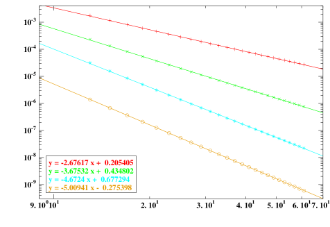
Figure 1: Numerical errors $\|u_{N}-u\|_{H^{1}}$ ($+$), $\|u_{N}-u\|_{L^{2}}$ ($\times$), $\|u_{N}-u\|_{H^{-1}}$ ($\ast$), and $|\lambda_{N}-\lambda|$ ($\circ$), as functions of $2N+1$ (the dimension of $\widetilde{X}_{N}$) in log scales.

4 Finite element discretization

In this section, we consider the problem

$$\inf\left\{E(v),\;v\in X,\;\int_{\Omega}v^{2}=1\right\},$$ (57)

where

$$\Omega\textrm{ is a rectangular brick of }\mathbb{R}^{d},\quad\mbox{with $d=1$, $2$ or $3$,}$$

$$X=H^{1}_{0}(\Omega),$$

$$E(v)=\frac{1}{2}\int_{\Omega}|\nabla v|^{2}+\frac{1}{2}\int_{\Omega}Vv^{2}+\frac{1}{2}\int_{\Omega}F(v^{2}).$$

We assume that $V\in L^{2}(\Omega)$ and that the function $F$ satisfies (7)-(7), as well as (8) for some $1<r\leq 2$ and $0\leq r+s\leq 3$. Throughout this section, we denote by $u$ the unique positive solution of (57) and by $\lambda$ the corresponding Lagrange multiplier.

In the non periodic case considered here, a classical variational approximation of (1) is provided by the finite element method. We consider a family of regular triangulations $({\cal T}_{h})_{h}$ of $\Omega$. This means, in the case when $d=3$ for instance, that for each $h>0$, ${\cal T}_{h}$ is a collection of tetrahedra such that

• $\overline{\Omega}$ is the union of all the elements of ${\cal T}_{h}$;

• the intersection of two different elements of ${\cal T}_{h}$ is either empty, a vertex, a whole edge, or a whole face of both of them;

• the ratio of the diameter $h_{K}$ of any element $K$ of ${\cal T}_{h}$ to the diameter of its inscribed sphere is smaller than a constant independent of $h$.

As usual, $h$ denotes the maximum of the diameters $h_{K}$, $K\in{\cal T}_{h}$. The parameter of the discretization then is $\delta=h>0$. For each $K$ in ${\cal T}_{h}$ and each nonnegative integer $k$, we denote by $\mathbb{P}_{k}(K)$ the space of the restrictions to $K$ of the polynomials with $d$ variables and total degree lower or equal to $k$.

The finite element space $X_{h,k}$ constructed from ${\cal T}_{h}$ and $\mathbb{P}_{k}(K)$ is the space of all continuous functions on $\Omega$ vanishing on $\partial\Omega$ such that their restrictions to any element $K$ of ${\cal T}_{h}$ belong to $\mathbb{P}_{k}(K)$. Recall that $X_{h,k}\subset H^{1}_{0}(\Omega)$ as soon as $k\geq 1$.

We denote by $\pi_{h,k}^{0}$ and $\pi_{h,k}^{1}$ the orthogonal projectors on $X_{h,k}$ for the $L^{2}$ and $H^{1}$ inner products respectively. The following estimates are classical (see e.g. [8]): there exists $C\in\mathbb{R}_{+}$ such that for all $r\in\mathbb{N}$ such that $1\leq r\leq k+1$,

$$\forall\phi\in H^{r}(\Omega)\cap H^{1}_{0}(\Omega), \|\phi-\pi_{h,k}^{0}\phi\|_{L^{2}}\leq Ch^{r}\|\phi\|_{H^{r}},$$

$$\forall\phi\in H^{r}(\Omega)\cap H^{1}_{0}(\Omega), \|\phi-\pi_{h,k}^{1}\phi\|_{H^{1}}\leq Ch^{r-1}\|\phi\|_{H^{r}}.$$ (58)

Let $u_{h,k}$ be a solution to the variational problem

$$\inf\left\{E(v_{h,k}),\;v_{h,k}\in X_{h,k},\;\int_{\Omega}v_{h,k}^{2}=1\right\}$$

such that $(u_{h,k},u)_{L^{2}}\geq 0$. In this setting, we obtain the following a priori error estimates.

Theorem 3

Assume that $V\in L^{2}(\Omega)$ and that the function $F$ satisfies (7), (7) for $q=1$, (7), and (8) for some $1<r\leq 2$ and $0\leq r+s\leq 3$. Then there exists $h_{0}>0$ and $C\in\mathbb{R}_{+}$ such that for all $0<h\leq h_{0}$,

$$\|u_{h,1}-u\|_{H^{1}} \leq C\,h$$ (59)

$$\|u_{h,1}-u\|_{L^{2}} \leq C\,h^{2}$$ (60)

$$|\lambda_{h,1}-\lambda| \leq C\,h^{2}$$ (61)

$$\frac{\gamma}{2}\|u_{h,1}-u\|_{H^{1}}^{2}\leq E(u_{h,1})-E(u) \leq C\,h^{2}.$$ (62)

If in addition, $V\in H^{1}(\Omega)$, $F$ satisfies (8) for $r=2$ and is such that $F\in C^{3}((0,+\infty),\mathbb{R})$ and $F^{\prime\prime}(t)t^{1/2}$ and $F^{\prime\prime\prime}(t)t^{3/2}$ are bounded in the vicinity of $0$, then there exists $h_{0}>0$ and $C\in\mathbb{R}_{+}$ such that for all $0<h\leq h_{0}$,

$$\|u_{h,2}-u\|_{H^{1}} \leq C\,h^{2}$$ (63)

$$\|u_{h,2}-u\|_{L^{2}} \leq C\,h^{3}$$ (64)

$$|\lambda_{h,2}-\lambda| \leq C\,h^{4}$$ (65)

$$\frac{\gamma}{2}\|u_{h,2}-u\|_{H^{1}}^{2}\leq E(u_{h,2})-E(u) \leq C\,h^{4}.$$ (66)

Proof

As $\Omega$ is a rectangular brick, $V$ satisfies (4) and $F$ satisfies (7)-(7), we have $u\in H^{2}(\Omega)$. We then use the fact that $\psi_{u_{h,k}-u}$ is solution to

$$-\Delta\psi_{u_{h,k}-u}+(V+f(u^{2})+2f^{\prime}(u^{2})u^{2}-\lambda)\psi_{u_{h,k}-u}$$

$$\qquad\qquad=2\left(\int_{\Omega}f^{\prime}(u^{2})u^{3}\psi_{u_{h,k}-u}\right)u+(u_{h,k}-u)-(u_{h,k}-u,u)_{L^{2}}u,\qquad\qquad$$

to establish that $\psi_{u_{h,k}-u}\in H^{2}(\Omega)\cap H^{1}_{0}(\Omega)$ and that

$$\|\psi_{u_{h,k}-u}\|_{H^{2}}\leq C\|u_{h,k}-u\|_{L^{2}}$$ (67)

for some constant $C$ independent of $h$ and $k$. The estimates (59)-(62) then are directly consequences of Theorem 1, (30), (58) and (67).

Under the additional assumptions that $V\in H^{1}(\Omega)$, we obtain by standard elliptic regularity arguments that $u\in H^{3}(\Omega)$. The $H^{1}$ and $L^{2}$ estimates (63) and (64) immediately follows from Theorem 1, (30), (58) and (67). We also have

$$|\lambda_{2,h}-\lambda|\leq Ch^{3}$$

for a constant $C$ independent of $h$. In order to prove (65), we proceed as in Section 3. We start from the equality

$$\lambda_{2,h}-\lambda=\langle(A_{u}-\lambda)(u_{2,h}-u),(u_{2,h}-u)\rangle_{X^{\prime},X}+\int_{\Omega}\widetilde{w}^{h}(u_{2,h}-u)$$

where

$$\widetilde{w}^{h}=u_{2,h}^{2}\frac{f(u_{2,h}^{2})-f(u^{2})}{u_{2,h}-u}.$$

We now claim that $u_{h,2}$ converges to $u$ in $L^{\infty}(\Omega)$ when $h$ goes to zero. To establish this result, we first remark that

$$\|u_{h,2}-u\|_{L^{\infty}}\leq\|u_{h,2}-{\cal I}_{h,2}u\|_{L^{\infty}}+\|{\cal I}_{h,2}u-u\|_{L^{\infty}},$$

where ${\cal I}_{h,2}$ is the interpolation projector on $X_{h,2}$. As $u\in H^{3}(\Omega)\hookrightarrow C^{1}(\overline{\Omega})$, we have

$$\lim_{h\to 0^{+}}\|{\cal I}_{h,2}u-u\|_{L^{\infty}}=0.$$

On the other hand, using the inverse inequality

$$\exists C\in\mathbb{R}_{+}\mbox{ s.t. }\forall 0<h\leq h_{0},\;\forall v_{h}\in X_{h,2},\quad\|v_{h,2}\|_{L^{\infty}}\leq C\rho(h)\|v_{h,2}\|_{H^{1}},$$

with $\rho(h)=1$ if $d=1$, $\rho(h)=1+\ln h$ if $d=2$ and $\rho(h)=h^{-1/2}$ if $d=3$ (see [8] for instance), we obtain

$$\|u_{h,2}-{\cal I}_{h,2}u\|_{L^{\infty}} \leq C\rho(h)\|u_{h,2}-{\cal I}_{h,2}u\|_{H^{1}}$$

$$\leq C\rho(h)\left(\|u_{h,2}-u\|_{H^{1}}+\|u-{\cal I}_{h,2}u\|_{H^{1}}\right)$$

$$\leq C^{\prime}\,\rho(h)\,h^{2}\;\mathop{\longrightarrow}_{h\to 0^{+}}\;0.$$

Hence the announced result. This implies in particular that $\widetilde{w}^{h}$ is bounded in $H^{1}(\Omega)$, uniformly in $h$. Consequently, there exists $C\in\mathbb{R}_{+}$ such that for all $0<h\leq h_{0}$,

$$|\lambda_{h,2}-\lambda|\leq C\left(\|u_{h,2}-u\|_{H^{1}}^{2}+\|u_{h,2}-u\|_{H^{-1}}\right).$$ (68)

To estimate the $H^{-1}$-norm of $u_{h,2}-u$, we write that for all $w\in H^{1}_{0}(\Omega)$,

$$\!\!\!\!\!\!\!\!\!\!\!\!\int_{\Omega}w(u_{h,2}-u) = \langle(E^{\prime\prime}(u)-\lambda)(u_{h,2}-u),\pi^{1}_{X_{h,2}\cap u^{\perp}}\psi_{w}\rangle_{X^{\prime},X}$$

$$+\langle(E^{\prime\prime}(u)-\lambda)(u_{h,2}-u),\psi_{w}-\pi^{1}_{X_{h,2}\cap u^{\perp}}\psi_{w}\rangle_{X^{\prime},X}$$

$$+\|u_{h,2}-u\|_{L^{2}}^{2}\int_{\Omega}f^{\prime}(u^{2})u^{3}\psi_{w}-\frac{1}{2}\|u_{h,2}-u\|_{L^{2}}^{2}\int_{\Omega}uw,$$

where $\psi_{w}$ is solution to

$$-\Delta\psi_{w}+(V+f(u^{2})+2f^{\prime}(u^{2})u^{2}-\lambda)\psi_{w}$$

$$\qquad\qquad=2\left(\int_{\Omega}f^{\prime}(u^{2})u^{3}\psi_{w}\right)u+w-(w,u)_{L^{2}}u,\qquad\qquad$$ (69)

and where $\pi^{1}_{X_{h,2}\cap u^{\perp}}$ denotes the orthogonal projector on $X_{h,2}\cap u^{\perp}$ for the $H^{1}$ inner product. Using the assumptions that $V\in H^{1}(\Omega)$, $F\in C^{3}((0,+\infty),\mathbb{R})$, and $F^{\prime\prime}(t)t^{1/2}$ and $F^{\prime\prime\prime}(t)t^{3/2}$ are bounded in the vicinity of $0$, we deduce from (69) that $\psi_{w}$ is in $H^{3}(\Omega)$ and that there exists $C\in\mathbb{R}_{+}$ such that for all $w\in H^{1}_{0}(\Omega)$ and all $0<h\leq h_{0}$,

$$\|\psi_{w}\|_{H^{3}}\leq C\|w\|_{H^{1}}.$$

We therefore obtain the inequality

$$\|\psi_{w}-\pi^{1}_{h,2}\psi_{w}\|_{H^{1}}\leq Ch^{2}\|w\|_{H^{1}},$$ (70)

where the constant $C$ is independent of $h$.

Putting together (8) (for $r=2$), (18), (38), (39), (58), (63), (64) and (70), we get

$$\|u_{h,2}-u\|_{H^{-1}}=\sup_{w\in H^{1}_{0}(\Omega)\setminus\left\{0\right\}}\frac{\int_{\Omega}w(u_{h,2}-u)}{\|w\|_{H^{1}}}\leq C\,h^{4}.$$

Combining with (63) and (68), we end up with (65). Lastly, we deduce (66) from the equality

$$E(u_{h,2})-E(u) = \frac{1}{2}\langle(A_{u}-\lambda)(u_{h,2}-u),(u_{h,2}-u)\rangle_{X^{\prime},X}$$

$$+\frac{1}{2}\int_{\Omega}F\left(u^{2}+(u_{h,2}^{2}-u^{2})\right)-F\left(u^{2}\right)-f\left(u^{2}\right)(u_{h,2}^{2}-u^{2}),$$

Taylor expanding the integrand and exploiting the boundedness of the function $F^{\prime\prime}(t)t^{1/2}$ in the vicinity of $0$.   $\Box$

Numerical results for the case when $\Omega=(0,\pi)^{2}$, $V(x_{1},x_{2})=x_{1}^{2}+x_{2}^{2}$ and $F(t^{2})=t^{2}/2$ are reported on Figure 2. The agreement with the error estimates obtained in Theorem 3 is good for the $\mathbb{P}_{1}$ approximation and excellent for the $\mathbb{P}_{2}$ approximation.

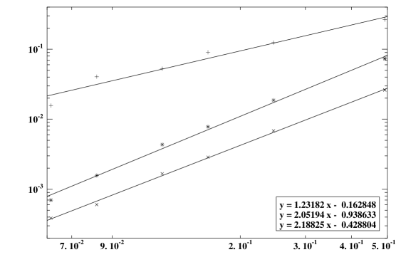
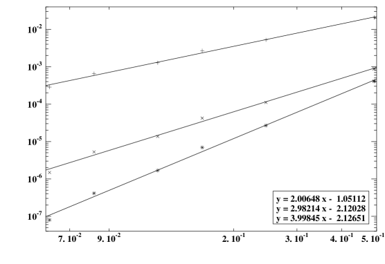
Figure 2: Errors $\|u_{h,k}-u\|_{H^{1}}$ ($+$), $\|u_{h,k}-u\|_{L^{2}}$ ($\times$) and $|\lambda_{h,k}-\lambda|$ ($\ast$) for the $\mathbb{P}_{1}$ ($k=1$, top) and $\mathbb{P}_{2}$ ($k=2$, bottom) approximations as a function of $h$ in log scales.

5 The effect of numerical integration

Let us now address one further consideration that is related to the practical implementation of the method, and more precisely to the numerical integration of the nonlinear term. For simplicity, we focus on the case when $A=1$.

From a practical viewpoint, the solution $(u_{\delta},\lambda_{\delta})$ to the nonlinear eigenvalue problem (15) can be computed iteratively, using for instance the optimal damping algorithm [4, 2, 7]. At the $p^{\rm th}$ iteration ($p\geq 1$), the ground state $(u_{\delta}^{p},\lambda_{\delta}^{p})\in X_{\delta}\times\mathbb{R}$ of some linear, finite dimensional, eigenvalue problem of the form

$$\int_{\Omega}\overline{\nabla u^{p}_{\delta}}\cdot\nabla v_{\delta}+\int_{\Omega}\left(V+f(\widetilde{\rho}_{\delta}^{p-1})\right)\,\overline{u_{\delta}^{p}}\,v_{\delta}=\lambda_{\delta}^{p}\int_{\Omega}\overline{u_{\delta}^{p}}v_{\delta},\quad\forall v_{\delta}\in X_{\delta},$$ (71)

has to be computed. In the optimal damping algorithm, the density $\widetilde{\rho}_{\delta}^{p-1}$ is a convex linear combination of the densites $\rho_{\delta}^{q}=|u^{q}_{\delta}|^{2}$, for $0\leq q\leq p-1$. Solving (71) amounts to finding the lowest eigenelement of the matrix $H^{p}$ with entries

$$H^{p}_{kl}:=\int_{\Omega}\overline{\nabla\phi_{k}}\cdot\nabla\phi_{l}+\int_{\Omega}V\,\overline{\phi_{k}}\,\phi_{l}+\int_{\Omega}f(\widetilde{\rho}_{\delta}^{p-1})\,\overline{\phi_{k}}\,\phi_{l},$$ (72)

where $(\phi_{k})_{1\leq k\leq\mbox{dim}(X_{\delta})}$ stands for the canonical basis of $X_{\delta}$.

In order to evaluate the last two terms of the right-hand side of (72), numerical integration has to be resorted to. In the finite element approximation of (57), it is generally made use of a numerical quadrature formula over each triangle (2D) or tetrahedron (3D) based on Gauss points. In the Fourier approximation of the periodic problem (40), the terms

$$\int_{\Omega}V\,\overline{e_{k}}\,e_{l}\quad\mbox{and}\quad\int_{\Omega}f(\widetilde{\rho}_{\delta}^{p-1})\,\overline{e_{k}}\,e_{l},$$

which are in fact, up to a multiplicative constant, the $(k-l)^{\rm th}$ Fourier coefficients of $V$ and $f(\widetilde{\rho}_{\delta}^{p-1})$ respectively, are evaluated by Fast Fourier Transform (FFT), using an integration grid which may be different from the natural discretization grid

$$\left\{\left(\frac{2\pi}{2N+1}j_{1},\cdots,\frac{2\pi}{2N+1}j_{d},\right),\;0\leq j_{1},\cdots,j_{d}\leq 2N\right\}$$

associated with $\widetilde{X}_{N}$. This raises the question of the influence of the numerical integration on the convergence results obtained in Theorems  1, 2 and 3.

Remark 4

In the case of the periodic problem considered in Section 3 and when $F(t)=ct^{2}$ for some $c>0$, the last term of the right-hand side of (72) can be computed exactly (up to round-off errors) by means of a Fast Fourier Transform (FFT) on an integration grid twice as fine as the discretization grid. This is due to the fact that the function $\widetilde{\rho}_{\delta}^{p-1}\,\overline{e_{k}}\,e_{l}$ belongs to the space $\mbox{Span}\{e_{n}\,|\,|n|_{*}\leq 4N\}$. An analogous property is used in the evaluation of the Coulomb term in the numerical simulation of the Kohn-Sham equations for periodic systems.

In the sequel, we focus on the simple case when $d=1$, $\Omega=(0,2\pi)$, $X=H^{1}_{\#}(0,2\pi)$, and

$$E(v)=\frac{1}{2}\int_{0}^{2\pi}|v^{\prime}|^{2}+\frac{1}{2}\int_{0}^{2\pi}Vv^{2}+\frac{1}{4}\int_{0}^{2\pi}|v|^{4}$$

with $V\in H^{\sigma}_{\#}(0,2\pi)$ for some $\sigma>1/2$. More difficult cases will be addressed elsewhere [5].

In view of Remark 4, we consider an integration grid

$$\frac{2\pi}{N_{g}}\mathbb{Z}\cap[0,2\pi)=\left\{0,\frac{2\pi}{N_{g}},\frac{4\pi}{N_{g}},\cdots,\frac{2\pi(N_{g}-1)}{N_{g}}\right\},$$

with $N_{g}\geq 4N+1$ for which we have

$$\forall v_{N}\in\widetilde{X}_{N},\quad\int_{0}^{2\pi}|v_{N}|^{4}=\frac{2\pi}{N_{g}}\sum_{r\in\frac{2\pi}{N_{g}}\mathbb{Z}\cap[0,2\pi)}|v_{N}(r)|^{4},$$

and for all $\rho\in\widetilde{X}_{2N}$,

$$\forall|k|,|l|\leq N,\quad\int_{0}^{2\pi}\rho\,\overline{e_{k}}\,e_{l}=\frac{1}{N_{g}}\sum_{r\in\frac{2\pi}{N_{g}}\mathbb{Z}\cap[0,2\pi)}\rho(r)e^{-i(k-l)r}=\widehat{\rho^{{\rm FFT}}_{k-l}},$$ (73)

where $\widehat{\rho^{{\rm FFT}}_{k-l}}$ is the $(k-l)^{\rm th}$ coefficient of the discrete Fourier transform of $\rho$. Recall that if $\phi=\sum_{g\in\mathbb{Z}}\widehat{\phi}_{g}\,e_{g}\in C^{0}_{\#}(0,2\pi)$, the discrete Fourier transform of $\phi$ is the $N_{g}\mathbb{Z}$-periodic sequence $(\widehat{\phi^{{\rm FFT}}_{g}})_{g\in\mathbb{Z}}$ defined by

$$\forall g\in\mathbb{Z},\quad\widehat{\phi^{{\rm FFT}}_{g}}=\frac{1}{N_{g}}\sum_{r\in\frac{2\pi}{N_{g}}\mathbb{Z}\cap[0,2\pi)}\phi(r)e^{-igr}.$$

We now introduce the subspaces $W_{M}$ for $M\in\mathbb{N}^{\ast}$ such that $W_{M}=\widetilde{X}_{(M-1)/2}$ if $M$ is odd and $W_{M}=\widetilde{X}_{M/2-1}\oplus\mathbb{C}(e_{M/2}+e_{-M/2})$ is $M$ is even (note that $\mbox{dim}(W_{M})=M$ for all $M\in\mathbb{N}^{\ast}$). It is then possible to define an interpolation projector ${\cal I}_{N_{g}}$ from $C^{0}_{\#}(0,2\pi)$ onto $W_{N_{g}}$ by

$$\forall x\in\frac{2\pi}{N_{g}}\mathbb{Z}\cap[0,2\pi),\quad[{\cal I}_{N_{g}}(\phi)](x)=\phi(x).$$

The expansion of ${\cal I}_{N_{g}}(\phi)$ in the canonical basis of $W_{N_{g}}$ is given by

$${\cal I}_{N_{g}}(\phi)\;=\;\left|\begin{array}[]{lll}(2\pi)^{1/2}\displaystyle\sum_{|g|\leq(N_{g}-1)/2}\widehat{\phi^{{\rm FFT}}_{g}}\,e_{g}&&(N_{g}\mbox{ odd}),\\ (2\pi)^{1/2}\displaystyle\sum_{|g|\leq N_{g}/2-1}\widehat{\phi^{{\rm FFT}}_{g}}\,e_{g}+(2\pi)^{1/2}\widehat{\phi^{{\rm FFT}}_{N_{g}/2}}\,\left(\frac{e_{N_{g}/2}+e_{-N_{g}/2}}{2}\right)&&(N_{g}\mbox{ even}).\end{array}\right.$$

Under the condition that $N_{g}\geq 4N+1$, the following property holds: for all $\phi\in C^{0}_{\#}(0,2\pi)$,

$$\forall|k|,|l|\leq N,\quad\int_{0}^{2\pi}{\cal I}_{N_{g}}(\phi)\,\overline{e_{k}}\,e_{l}=\widehat{\phi^{{\rm FFT}}_{k-l}}.$$

It is therefore possible, in the particular case considered here, to efficiently evaluate the entries of the matrix $H^{p}$ using the formula

$$H^{p}_{kl} := \int_{0}^{2\pi}\overline{e_{k}^{\prime}}\cdot e_{l}^{\prime}+\int_{0}^{2\pi}V\,\overline{e_{k}}\,e_{l}+\int_{0}^{2\pi}\widetilde{\rho}_{N}^{p-1}\overline{e_{k}}\,e_{l}$$ (74)

$$\simeq |k|^{2}\delta_{kl}+\widehat{V^{{\rm FFT}}_{k-l}}+\widehat{[\widetilde{\rho}_{N}^{p-1}]^{\rm FFT}_{k-l}},$$

and resorting to Fast Fourier Transform (FFT) algorithms to compute the discrete Fourier transforms. Note that only the second term is computed approximatively. The third term is computed exactly since, at each iteration, $\widetilde{\rho}_{N}^{p-1}$ belongs to $\widetilde{X}_{2N}$ (see Eq. (73)). Of course, this situation is specific to the nonlinearity $F(t)=t^{2}/2$ considered here.

Using the approximation formula (74) amounts to replace the original problem

$$\inf\left\{E(v_{N}),\;v_{N}\in\widetilde{X}_{N},\;\int_{0}^{2\pi}|v_{N}|^{2}=1\right\},$$ (75)

with the approximate problem

$$\inf\left\{E_{N_{g}}(v_{N}),\;v_{N}\in\widetilde{X}_{N},\;\int_{0}^{2\pi}|v_{N}|^{2}=1\right\},$$ (76)

where

$$E_{N_{g}}(v_{N})=\frac{1}{2}\int_{0}^{2\pi}|v_{N}^{\prime}|^{2}+\frac{1}{2}\int_{0}^{2\pi}{\cal I}_{N_{g}}(V)v_{N}^{2}+\frac{1}{4}\int_{0}^{2\pi}|v_{N}|^{4}.$$

Let us denote by $u_{N}$ a solution of (75) such that $(u_{N},u)_{L^{2}}\geq 0$ and by $u_{N,N_{g}}$ a solution to (76) such that $(u_{N,N_{g}},u)_{L^{2}}\geq 0$. It is easy to check that $u_{N,N_{g}}$ is bounded in $H^{1}_{\#}(0,2\pi)$ uniformly in $N$ and $N_{g}$.

Besides, we know from Theorem 2 that $(u_{N})_{N\in\mathbb{N}}$ converges to $u$ in $H^{1}_{\#}(0,2\pi)$, hence in $L^{\infty}_{\#}(2,\pi)$, when $N$ goes to infinity. This implies that the sequence $(A_{u}-A_{u_{N}})_{N\in\mathbb{N}}$ converges to $0$ in operator norm. Consequently, for all $N$ large enough and all $N_{g}$ such that $N_{g}\geq 4N+1$,

$$\frac{\gamma}{4}\|u_{N,N_{g}}-u_{N}\|_{H^{1}}^{2} \leq E(u_{N,N_{g}})-E(u_{N})$$

$$\leq E_{N_{g}}(u_{N,N_{g}})-E_{N_{g}}(u_{N})$$

$$+\int_{0}^{2\pi}(V-{\cal I}_{N_{g}}(V))\left(|u_{N,N_{g}}|^{2}-|u_{N}|^{2}\right)$$

$$\leq \int_{0}^{2\pi}(V-{\cal I}_{N_{g}}(V))\left(|u_{N,N_{g}}|^{2}-|u_{N}|^{2}\right)$$

$$\leq C\|\Pi_{2N}(V-{\cal I}_{N_{g}}(V))\|_{L^{2}}\|u_{N,N_{g}}-u_{N}\|_{H^{1}},$$

where we have used the fact that $\left(|u_{N,N_{g}}|^{2}-|u_{N}|^{2}\right)\in\widetilde{X}_{2N}$. Therefore,

$$\|u_{N,N_{g}}-u_{N}\|_{H^{1}}\leq C\|\Pi_{2N}(V-{\cal I}_{N_{g}}(V))\|_{L^{2}},$$ (77)

for a constant $C$ independent of $N$ and $N_{g}$. Likewise,

$$\lambda_{N,N_{g}}-\lambda_{N} = \langle(A_{u_{N}}-\lambda_{N})(u_{N,N_{g}}-u_{N}),(u_{N,N_{g}}-u_{N})\rangle_{X^{\prime},X}$$

$$+\int_{0}^{2\pi}(V-{\cal I}_{N}(V))|u_{N,N_{g}}|^{2}$$

$$+\int_{0}^{2\pi}|u_{N,N_{g}}|^{2}(u_{N,N_{g}}+u_{N})(u_{N,N_{g}}-u_{N}),$$

from which we deduce, using (77),

$$|\lambda_{N,N_{g}}-\lambda_{N}|\leq C\|\Pi_{2N}(V-{\cal I}_{N_{g}}(V))\|_{L^{2}}.$$

An error analysis of the interpolation operator ${\cal I}_{N_{g}}$ is given in [6]: for all non-negative real numbers $0\leq r\leq s$ with $s>1/2$ (for $d=1$),

$$\|\varphi-{\cal I}_{N_{g}}(\varphi)\|_{H^{r}}\leq\frac{C}{N_{g}^{s-r}}\|\varphi\|_{H^{s}},\quad\forall\varphi\in H^{s}_{\#}(0,2\pi).$$

Thus,

$$\|\Pi_{2N}(V-{\cal I}_{N_{g}}(V))\|_{L^{2}}\leq\|V-{\cal I}_{N_{g}}(V)\|_{L^{2}}\leq\frac{C}{N_{g}^{\sigma}},$$ (78)

and the above inequality provides the following estimates:

$$\|u_{N,N_{g}}-u\|_{H^{1}} \leq C\left(N^{-\sigma-1}+N_{g}^{-\sigma}\right)$$ (79)

$$\|u_{N,N_{g}}-u\|_{L^{2}} \leq C\left(N^{-\sigma-2}+N_{g}^{-\sigma}\right)$$ (80)

$$|\lambda_{N,N_{g}}-\lambda| \leq C\left(N^{-2\sigma-2}+N_{g}^{-\sigma}\right),$$ (81)

for a constant $C$ independent of $N$ and $N_{g}$. The first component of the error bound (79) corresponds to the error $\|u_{N}-u\|_{H^{1}}$ while the second component corresponds to the numerical integration error $\|u_{N,N_{g}}-u_{N}\|_{H^{1}}$ (the same remark applies to the error bounds (80) and (81)).

It is classical that for the norm $\|\varphi-{\cal I}_{N_{g}}\varphi\|_{H^{r}}$ for $r<0$ is in general of the same order of magnitude as $\|\varphi-{\cal I}_{N_{g}}\varphi\|_{L^{2}}$. As the existence of better estimates in negative norms is a corner stone in the derivation of the improvement of the error estimate (46) for the eigenvalues (doubling of the convergence rate), we expect that the eigenvalue approximation will be dramatically polluted by the use of the numerical integration formula.

This can be checked numerically. Considering again the one-dimensional example used in Section 3 ($\Omega=(0,2\pi)$, $V(x)=\sin(|x-\pi|/2)$, $F(t)=t^{2}/2$), we have computed for $4\leq N\leq 30$ and $N_{g}=2^{p}$ with $7\leq p\leq 15$, the errors $\|u_{N,N_{g}}-u\|_{H^{1}}$, $\|u_{N,N_{g}}-u\|_{L^{2}}$, $\|u_{N,N_{g}}-u\|_{H^{-1}}$, and $|\lambda_{N,N_{g}}-\lambda|$. On Figure 3, these quantities are plotted as functions of $2N+1$ (the dimension of $\widetilde{X}_{N}$), for various values of $N_{g}$.

The non-monotonicity of the curve $N\mapsto|\lambda_{N,N_{g}}-\lambda|$ originates from the fact that $\lambda_{N,N_{g}}-\lambda$ can be positive or negative depending on the values of $N$ and $N_{g}$.

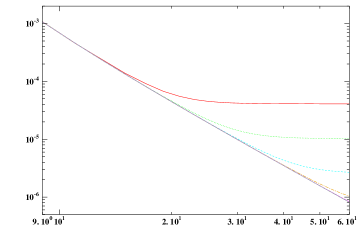
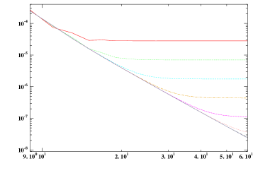
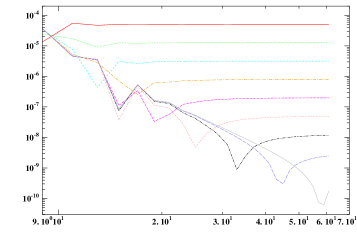
Figure 3: Numerical errors $\|u_{N,N_{g}}-u\|_{H^{1}}$ (top left), $\|u_{N,N_{g}}-u\|_{L^{2}}$ (top right), $\|u_{N,N_{g}}-u\|_{H^{-1}}$ (bottom left), and $|\lambda_{N,N_{g}}-\lambda|$ (bottom right), as functions of $2N+1$ (the dimension of $\widetilde{X}_{N}$), for $N_{g}=128$ (red), $N_{g}=256$ (green), $N_{g}=512$ (cyan), $N_{g}=1024$ (gold), $N_{g}=2048$ (magenta), $N_{g}=4096$ (pink), $N_{g}=8192$ (black), $N_{g}=16384$ (blue), $N_{g}=32768$ (light blue).

The numerical errors $\|u_{N,N_{g}}-u\|_{H^{1}}$, $\|u_{N,N_{g}}-u\|_{L^{2}}$, $\|u_{N,N_{g}}-u\|_{H^{-1}}$, and $|\lambda_{N,N_{g}}-\lambda|$, for $N=30$, as functions of $N_{g}$ (in log scales) are plotted on Figure 4. When $N_{g}$ goes to infinity, the sequences $\log_{10}\|u_{N,N_{g}}-u\|_{H^{1}}$, $\log_{10}\|u_{N,N_{g}}-u\|_{L^{2}}$, $\log_{10}\|u_{N,N_{g}}-u\|_{H^{-1}}$, and $\log_{10}|\lambda_{N,N_{g}}-\lambda|$ converge to $\log_{10}\|u_{N}-u\|_{H^{1}}$, $\log_{10}\|u_{N}-u\|_{L^{2}}$, $\log_{10}\|u_{N}-u\|_{H^{-1}}$, and $\log_{10}|\lambda_{N}-\lambda|$ respectively. For smaller values of $N_{g}$, the numerical integration error dominates and these functions all decay linearly with $\log_{10}N_{g}$ with a slope very close to $-2$. For fixed $N$, the upper bounds (79)-(81) also decay linearly with $\log_{10}N_{g}$, but with a slope equal to $-1.5$. To obtain sharper upper bounds for the numerical integration error, we need to replace (78) with a sharper estimate of $\|\Pi_{2N}(V-{\cal I}_{N_{g}}(V))\|_{L^{2}}$, which is possible for the particular example under consideration here. Indeed, remarking that under the condition $N_{g}\geq 4N+1$,

$$\|\Pi_{2N}(V-{\cal I}_{N_{g}}(V))\|_{L^{2}}=\left(\sum_{|g|\leq 2N}\left|\sum_{k\in\mathbb{Z}^{\ast}}\widehat{V}_{g+kN_{g}}\right|^{2}\right)^{1/2},$$

we can, using (56), show that

$$\|\Pi_{2N}(V-{\cal I}_{N_{g}}(V))\|_{L^{2}}\leq\frac{C\,N^{1/2}}{N_{g}^{2}},$$

for a constant $C$ independent of $N$ and $N_{g}$. We deduce that for this specific example

$$\|u_{N,N_{g}}-u\|_{H^{1}} \leq C\left(N^{-5/2}+N^{1/2}N_{g}^{-2}\right)$$

$$\|u_{N,N_{g}}-u\|_{L^{2}} \leq C\left(N^{-7/2}+N^{1/2}N_{g}^{-2}\right)$$

$$|\lambda_{N,N_{g}}-\lambda| \leq C\left(N^{-9/2}+N^{1/2}N_{g}^{-2}\right).$$

Figure 4: Numerical errors $\|u_{N,N_{g}}-u\|_{H^{1}}$ ($\times$), $\|u_{N,N_{g}}-u\|_{L^{2}}$ ($+$), $\|u_{N,N_{g}}-u\|_{H^{-1}}$ ($\ast$), and $|\lambda_{N,N_{g}}-\lambda|$ ($\circ$), for $N=30$, as functions of $N_{g}$ (in log scales).

6 Appendix: properties of the ground state

The mathematical properties of the minimization problems (1) and (9) which are useful for the numerical analysis reported in this article are gathered in the following lemma.

Recall that $d=1$, $2$ or $3$.

Lemma 2

Under assumptions (3)-(7), (9) has a unique minimizer $\rho_{0}$ and (1) has exactly two minimizers $u=\sqrt{\rho_{0}}$ and $-u$. The function $u$ is solution to the nonlinear eigenvalue problem (11) for some $\lambda\in\mathbb{R}$. Besides, $u\in C^{0,\alpha}(\overline{\Omega})$ for some $0<\alpha<1$, $u>0$ in $\Omega$, and $\lambda$ is the lowest eigenvalue of $A_{u}$ and is non-degenerate.

Proof

As $A$ is uniformly bounded and coercive on $\Omega$ and $V\in L^{q}(\Omega)$ for some $q>\max(1,d/2)$, $v\mapsto a(v,v)$ is a quadratic form on $X$, bounded from below on the set $\left\{v\in X\;|\;\|v\|_{L^{2}}=1\right\}$. Replacing $a(v,v)$ with $a(v,v)+C\|v\|_{L^{2}}^{2}$ and $F(t)$ with $F(t)-F(0)-tF^{\prime}(0)$ does not change the minimizers of (1) and (9). We can therefore assume, without loss of generality, that

$$\forall v\in X,\;a(v,v)\geq\|v\|_{L^{2}}^{2}\quad\mbox{ and }\quad F(0)=F^{\prime}(0)=0.$$ (82)

It then follows from (7) and (82) that $0\leq F(v^{2})\leq C(v^{2}+v^{6})$. As $X\hookrightarrow L^{6}(\Omega)$, $E(v)$ is finite for all $v\in X$, $I>-\infty$ and the minimizing sequences of (1) are bounded in $X$. Let $(v_{n})_{n\in\mathbb{N}}$ be a minimizing sequence of (1). Using the fact that $X$ is compactly embedded in $L^{2}(\Omega)$, we can extract from $(v_{n})_{n\in\mathbb{N}}$ a subsequence $(v_{n_{k}})_{k\in\mathbb{N}}$ which converges weakly in $X$, strongly in $L^{2}(\Omega)$ and almost everywhere in $\Omega$ to some $u\in X$. As $\|v_{n_{k}}\|_{L^{2}}=1$ and $E(v_{n_{k}})\downarrow I$, we obtain $\|u\|_{L^{2}}=1$ and $E(u)\leq I$ ($E$ is convex and strongly continuous, hence weakly l.s.c., on $X$). Hence $u$ is a minimizer of (1). As $|u|\in X$, $\||u|\|_{L^{2}}=1$ and $E(|u|)=E(u)$, we can assume without loss of generality that $u\geq 0$. Assumptions (3)-(7) imply that $E$ is $C^{1}$ on $X$ and that $E^{\prime}(u)=A_{u}u$. It follows that $u$ is solution to (10) for some $\lambda\in\mathbb{R}$. By elliptic regularity arguments [10], we get $u\in C^{0,\alpha}(\overline{\Omega})$ for some $0<\alpha<1$. We also have $u>0$ in $\Omega$; this is a consequence of the Harnack inequality [12]. Making the change of variable $\rho=v^{2}$, it is easily seen that if $v$ is a minimizer of (1), then $v^{2}$ is a minimizer of (9), and that, conversely, if $\rho$ is a minimizer of (9), then $\sqrt{\rho}$ and $-\sqrt{\rho}$ are minimizers of (1). Besides, the functional $\cal E$ is strictly convex on the convex set $\left\{\rho\geq 0\;|\,\sqrt{\rho}\in X,\;\int_{\Omega}\rho=1\right\}$. Therefore $\rho_{0}=u^{2}$ is the unique minimizer of (9) and $u$ and $-u$ are the only minimizers of (1).

It is easy to see that $A_{u}$ is bounded below and has a compact resolvent. It therefore possesses a lowest eigenvalue $\lambda_{0}$, which, according to the min-max principle, satisfies

$$\lambda_{0}=\inf\left\{\int_{\Omega}(A\nabla v)\cdot\nabla v+\int_{\Omega}(V+f(u^{2}))v^{2},\;v\in X,\;\int_{\Omega}v^{2}=1\right\}.$$ (83)

Let $v_{0}$ be a normalized eigenvector of $A_{u}$ associated with $\lambda_{0}$. Clearly, $v_{0}$ is a minimizer of (83) and so is $|v_{0}|$. Therefore, $|v_{0}|$ is solution to the Euler equation $A_{u}|v_{0}|=\lambda_{0}|v_{0}|$. Using again elliptic regularity arguments and the Harnack inequality, we obtain that $|v_{0}|\in C^{0,\alpha}(\overline{\Omega})$ for some $0<\alpha<1$ and that $|v_{0}|>0$ on $\Omega$. This implies that either $v_{0}=|v_{0}|>0$ in $\Omega$ or $v_{0}=-|v_{0}|<0$ in $\Omega$. In particular $(u,v_{0})_{L^{2}}\neq 0$. Consequently, $\lambda=\lambda_{0}$ and $\lambda$ is a simple eigenvalue of $A_{u}$.   $\Box$

Let us finally prove that $\lambda$ is also the ground state eigenvalue of the nonlinear eigenvalue problem

$$\left\{\begin{array}[]{l}\mbox{search }(\mu,v)\in\mathbb{R}\times X\mbox{ such that}\\ A_{v}v=\mu v\\ \|v\|_{L^{2}}=1,\end{array}\right.$$ (84)

in the following sense: if $(\mu,v)$ is solution to (84) then either $\mu>\lambda$ or $\mu=\lambda$ and $v=\pm u$.

To see this, let us consider a solution $(\mu,v)\in\mathbb{R}\times X$ to (84) and denote by $\widetilde{w}=|v|-u$. As for $u$, we infer from elliptic regularity arguments [10] that $v\in C^{0,\alpha}(\overline{\Omega})$. We have $\|v\|_{L^{2}}=\|u\|_{L^{2}}=1$. Therefore, if $w\leq 0$ in $\Omega$, then $|v|=u$, which yields $v=\pm u$ and $\mu=\lambda$. Otherwise, there exists $x_{0}\in\Omega$ such that $\widetilde{w}(x_{0})>0$, and, up to replacing $v$ with $-v$, we can consider that the function $w=v-u$ is such that $w(x_{0})>0$. The function $w$ is in $X\cap C^{0,\alpha}(\overline{\Omega})$ and satisfies

$$(A_{u}-\lambda)w+\frac{f(v^{2})-f(u^{2})}{v^{2}-u^{2}}v(u+v)w=(\mu-\lambda)v.$$ (85)

Let $\omega=\left\{x\in\Omega\;|\;w(x)>0\right\}=\left\{x\in\Omega\;|\;v(x)>u(x)\right\}$ and $w_{+}=\max(w,0)$. As $w_{+}\in X$, we deduce from (85) that

$$\langle(A_{u}-\lambda)w_{+},w_{+}\rangle_{X^{\prime},X}+\int_{\omega}\frac{f(v^{2})-f(u^{2})}{v^{2}-u^{2}}v(u+v)w^{2}=(\mu-\lambda)\int_{\omega}vw.$$

The left hand side of the above equality is positive and $\int_{\omega}vw>0$. Therefore, $\mu>\lambda$.

References

[1] I. Babuška and J. Osborn, Eigenvalue
problems, in: Handbook of numerical analysis. Volume II,
(North-Holland, 1991) 641-787.
[2] E. Cancès, SCF algorithms
for Kohn-Sham models with fractional occupation numbers,
J. Chem. Phys. 114 (2001) 10616-10623.
[3] E. Cancès, M. Defranceschi,
W. Kutzelnigg, C. Le Bris
and Y. Maday, Computational quantum chemistry: a primer, in:
Handbook of numerical analysis. Volume X: special volume:
computational chemistry, Ph. Ciarlet and C. Le Bris eds (North-Holland,
2003) 3-270.
[4] E. Cancès and
C. Le Bris, Can we outperform the DIIS approach for electronic
structure calculations?, Int. J. Quantum Chem. 79 (2000) 82-90.
[5] E. Cancès, R. Chakir and Y. Maday, Numerical
analysis of the planewave discretization of Kohn-Sham and related
models, in preparation.
[6] C. Canuto, M.Y. Hussaini, A. Quarteroni and T.A. Zang,
Spectral methods, Springer, 2007.
[7] C. Dion and E. Cancès, Spectral method for
the time-dependent Gross-Pitaevskii equation with harmonic traps,
Phys. Rev. E 67 (2003) 046706.
[8] A. Ern and J.-L. Guermond, Theory and practice of
finite elements, Springer, 2004.
[9] L. P. Pitaevskii and S. Stringari, Bose-Einstein
condensation, Clarendon Press, 2003.
[10] D. Gilbarg and N.S. Trudinger, Elliptic
partial differential equations of second order, 3rd edition, Springer
1998.
[11] W. Sickel, Superposition of functions in Sobolev
spaces of fractional order. A survey, Banach Center Publ. 27 (1992)
481-497.
[12] G. Stampacchia, Le problème de Dirichlet pour
les équations elliptiques du second ordre à coefficients
discontinues, Ann. Inst. Fourier, tome 15 (1965) 189-257.
[13] A. Zhou, An analysis of finite-dimensional
approximations for the ground state solution of Bose-Einstein
condensates, Nonlinearity 17 (2004) 541-550.
[14] A. Zhou, Finite dimensional approximations for the
electronic ground state solution of a molecular system,
Math. Meth. Appl. Sci. 30 (2007) 429-447.