Planetary transit observations at the University Observatory Jena: TrES-2

Abstract

We report on observations of several transit events of the transiting planet TrES-2 obtained with the Cassegrain-Telskop-Kamera at the University Observatory Jena. Between March 2007 and November 2008 ten different transits and almost a complete orbital period were observed. Overall, in 40 nights of observation 4291 exposures (in total 71.52 h of observation) of the TrES-2 parent star were taken. With the transit timings for TrES-2 from the 34 events published by the TrES-network, the Transit Light Curve project and the Exoplanet Transit Database plus our own ten transits, we find that the orbital period is $P=(2.470614\pm 0.000001)\,$d, a slight change by $\sim$ 0.6 s compared to the previously published period. We present new ephemeris for this transiting planet.
Furthermore, we found a second dip after the transit which could either be due to a blended variable star or occultation of a second star or even an additional object in the system.
Our observations will be useful for future investigations of timing variations caused by additional perturbing planets and/or stellar spots and/or moons.

1 Introduction

TrES-2 is the second transiting hot Jupiter discovered by the Trans-atlantic Exoplanet Survey (TrES, O’Donovan et al. 2006). The planet orbits the nearby 11th magnitude G0 V main-sequence dwarf GSC 03549-02811 every $\sim$2.5 days. From high-resolution spectra, Sozzetti et al. (2007) derived accurate values of the stellar atmospheric parameters of the TrES-2 parent star such as effective temperature, surface gravity and metallicity. With the help of detailed analysis of high precision z-band photometry and light curve modeling of the 1.4% deep transit by the Transit Light Curve (TLC) Project (Holman et al. 2007), estimates of the planetary parameters could also be determined.
One goal of the TLC project is to measure variations in the transit times and light curve shapes that would be caused by the influence of additional bodies in the system (Agol et al. 2005; Holman & Murray 2005; Steffen & Agol 2005). The large impact parameter of TrES-2 makes the duration more sensitive to any changes. Hence, TrES-2 is an excellent target for the detection of long-term changes in transit characteristics induced by orbital precession (Miralda-Escudé 2002).
We have started high precision photometric observations at the University Observatory Jena in fall 2006. In this work we use the transit method to observe the transiting planet TrES-2. We paid special attention to the accurate determination of transit times in order to identify precise transit timing variations that would be indicative of perturbations from additional bodies and to refine the orbital parameters of the system. First results were presented in Raetz et al. (2009a).
TrES-2 lies within the field of view of the NASA Kepler mission (Borucki et al 2003; Basri et al 2005). During the four year mission, Kepler will observe nearly 600 transits of TrES-2 (O’Donovan et al. 2006). The precision of Kepler will be extremely sensitive to search for additional planets in the TrES-2 system through their dynamical perturbations.
In this paper, we describe the observations, the data reduction and the analysis procedures. Furthermore, we present results for TrES-2 that we obtained from our observations at the University Observatory Jena.

2 Observations

2.1 University Observatory Jena Photometry

Most observations were carried out at the University Observatory Jena which is located close to the village Groß- schwabhausen, 10 km west of the city of Jena.
Mugrauer (2009) describes the instrumentation and operation of the system. Our transit observations are carried out with the CTK (Cassegrain Teleskop Kamera), the CCD imager operated at the 25 cm auxiliary telescope of the University Observatory Jena.
The CTK CCD-detector consists of 1024 $\times$ 1024 pixel with a pixel scale of about 2.2 ${}^{\prime\prime}$/pixel which yields a field of view of 37.7 ${}^{\prime}\,\times\,$37.7 ${}^{\prime}$ (for more details see Mugrauer 2009).
We started our observations in November 2006. Between March 2007 and November 2008, we used 49 clear nights for our transit observations. Part of the time we observed known transiting planets in Bessell $R$ and $I$ band.
For our TrES-2 observations, started in March 2007, we used 43 nights from March 2007 to November 2008. Due to the weather conditions 3 nights were not useable. We observed nine different transits. These transits correspond to epochs 87, 108, 138, 163, 165, 174, 278, 316 and 318 of the ephemeris given by Holman et al. (2007):

$$\begin{array}[]{r@{.}lcr@{.}l}T_{\mathrm{c}}(E)=(2453957&63479&+&E\cdot 2&470621)\,\mathrm{d}\\ \pm 0&00038&&\pm 0&000017\end{array}$$ (3)

To get a phase diagram of one full orbital period, we observed TrES-2 even in times out of transit. All TrES-2 observations were taken in $I$-band with 60 s exposure time. We achieve a mean cadence of the data points of 1.4 min (readout time of the CTK around 24 s). The mean photometric precision of the $V\,\approx$ 11 mag bright TrES-2 host star is 0.007 mag. Fig. 1 shows the field of view of the CTK around the TrES-2 host star.

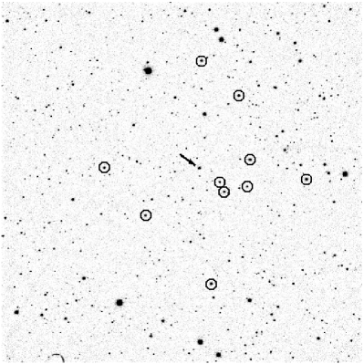
Figure 1: The 37.7 ${}^{\prime}\times$ 37.7 ${}^{\prime}$ field of view of the CTK ($I$-band, exposure time 60 s). The arrow marks the TrES-2 host star, the circles the 10 most constant comparison stars. North is up; east is to the left.

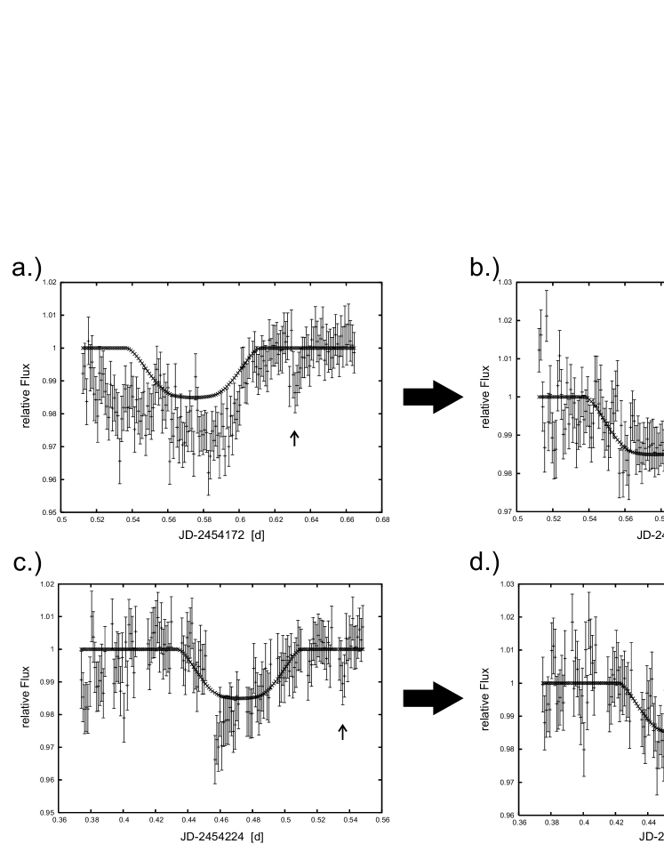
Figure 2: Two different transits of TrES-2 before and after using Sys-Rem. a.) The transit from 2007 March 13 before Sys-Rem b.) The transit from 2007 March 13 after Sys-Rem c.) The transit from 2007 May 3 before Sys-Rem d.) The transit from 2007 May 3 after Sys-Rem. The arrow marks the time of the second dip discussed in Section 7

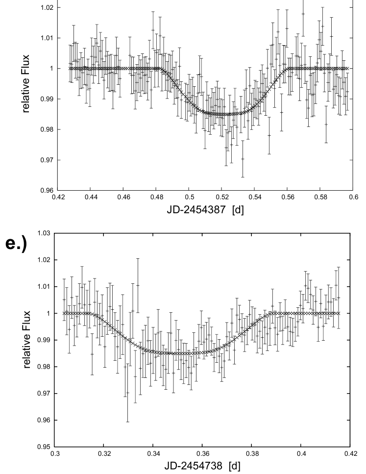
Figure 3: $I$ band photometry of six TrES-2-transits observed at the University Observatory Jena: a.) 2007 July 17 b.) 2007 September 21 c.) 2007 October 13 d.) 2008 June 26 e.) 2008 September 28 f.) 2008 October 3

2.2 Additional Photometry

In 2007 July and September, we observed two transit events at the Wendelstein Observatory of the university of Munich. The transits from 2007 July 26 and 2007 September 16 include 157 and 137 $R$-band 30 s exposures, respectively. According to the ephemeris provided by Holman et al. (2007), these transits correspond to epochs 142 and 163. All 294 images were acquired using the MONICA (MOno-chromatic Image CAmera, Roth 1990) CCD camera, at the Cassegrain focus of the 0.8 m Wendelstein telescope, with a pixel scale of 0.5 ${}^{\prime\prime}$/pixel and a field of view of 8.5${}^{\prime}\,\times$ 8.5${}^{\prime}$.
The pre-reduction was done using standard reduction software (MUPIPE) specifically developed at the Munich Observatory for the MONICA CCD camera (Gössl & Riffeser 2002). For these observations the mean photometric precision is 0.005 mag.
Because of the good weather conditions on 2007 September 16 we recruited an amateur astronomer (M.R.) to observe this transit of TrES-2. As Naeye (2004) and McCullough et al. (2006) showed, amateur astronomers can produce photometry with sufficient quality to detect a transit. With an 8-inch ($\sim$ 20 cm) Schmidt-Cassegrain telescope (f/D = 10) and a ST-6 CCD camera (field of view 13.6 ${}^{\prime}\,\times\,$10.2 ${}^{\prime}$) without filter (white-light observations) located in Herges-Hal- lenberg, Germany, we reached a photometric precision of 0.01 mag. With this observation we have three independent measurements of the transit from 2007 September 16 (epoch 163 according to eq. 3), see Fig. 4.

3 Data Reduction and analysis of time series

3.1 In general

We calibrate the images of our target field using the standard IRAF procedures darkcombine, flatcombine and ccdproc. We did not correct for bad pixel (see Raetz et al. 2009b).
First we perform aperture photometry by using the IRAF task chphot (see Raetz et al. 2009b).
For differential photometry we use an algorithm that calculates an artificial comparison star by taking the weighted average of a maximum number of stars (all available field stars). To compute the best possible artificial comparison star we successively sort out all stars with low weights (stars that are not on every image, stars with low S/N and variable stars). As result, we get an artificial comparison star made of the most constant stars with the best S/N in the field (Broeg et al. 2005, Raetz et al. 2009b).
In the third step we correct for systematic effects by using the Sys-Rem detrending algorithm which was developed by Tamuz et al. (2005) and implemented by Johannes Koppenhoefer, see Fig. 2. We showed in Raetz et al. (2009b) that the usage of Sys-Rem is not possible in every case of observations at the University Observatory Jena.

3.2 The case of TrES-2

After calibrating all images, we perform aperture photometry on all available field stars. We found 1294 stars - the TrES-2 host star and 1293 comparison stars - in the CTK field of view. We used an aperture of 5 pixels (11.03${}^{\prime\prime}$) radius and an annulus for sky subtraction ranging in radius from 15 to 20 pixels, centered on each star.
To get the best possible result for the transit light curves, we reject all comparison stars that could not be measured on every image, faint stars with low S/N and variable stars which could introduce disturbing signals to the data. We have done this analysis individually for every night. To get comparable values for every night, we search for those comparison stars that belong always to the most constant stars. Finally we use for every night the same 10 constant comparison stars to calculate the artificial comparison stars (see Fig. 1). With this method we could improve the preliminary results given in Raetz et al. (2009a).
For the Wendelstein observations we chose an aperture size of 10 pixels (5${}^{\prime\prime}$). And for sky subtraction we use a ring-shaped annulus having an inner/outer radius of 15/20 pixels, respectively. We were not able to use the same 10 comparison stas as in the case of observations at the University Observatory Jena because they do not lie within the 8.5${}^{\prime}\,\times$ 8.5${}^{\prime}$ field of view of MONICA. From 225 objects in this field we could calculate the artificial comparison star for both nights using the seven most constant stars.
For the amateur observations only 147 stars could be measured within an aperture of 5 pixels (11.8${}^{\prime\prime}$) and an annulus for sky substraction similar to observations at the University Observatory Jena and on Wendelstein. Again it was not possible to use the 10 best comparison stars froUniversity Observatory Jena observations or the seven comparison stars from Wendelstein observations. In this case the artificial comparison star consists of the 15 most contant stars in the ST-6 field.
Finally the TrES-2 host star is compared to the artificial comparison star to get the differential magnitudes for every image.
In the resulting light curves of the TrES-2 host star and the comparison stars we used Sys-Rem. The algorithm works without any prior knowledge of the effects. The number of effects that should be removed from the light curves is selectable and can be set as a parameter. As mentioned in section 3.1 it was not possible to use Sys-Rem for every night. In Table 1 we summarize how many effects we removed from the light curves by using Sys-Rem before the transit itself is identified as systematic effect. Zero means that we could not apply Sys-Rem. Fig. 2 shows for example the effect of Sys-Rem for two different transits of TrES-2.
The resulting light curves from the University Observatory Jena observations can be found in Fig. 3 and 4a, the Wendelstein observations in Fig. 4b and 5 and the amateur observations in Fig. 4c.

Table 1: Information of observations and analysis for all measured transit events

Date	Observatory	Transit	Points${}^{a}$	removed
				Effects${}^{b}$
2007 Mar 13	Jena	Full	96	1
2007 May 3	Jena	Full	75	1
2007 Jul 17	Jena	Partial	52	0
2007 Jul 26	Wendelstein	Full	76	0
2007 Sep 16	Jena	Full	78	1
2007 Sep 16	Wendelstein	Full	65	2
2007 Sep 16	Amateur	Full	75	1
2007 Sep 21	Jena	Partial	55	0
2007 Oct 13	Jena	Full	89	1
2008 Jun 26	Jena	Full	85	1
2008 Sep 28	Jena	Full	96	1
2008 Oct 03	Jena	Partial	43	0

${}^{a}$ Number of data points covering the transit; i.e., within the phases 0.98-1.02.
${}^{b}$ Number of effects that are removed from the light curves by using Sys-Rem

Table 2: Summary of all previously known and new transit times of TrES-2.

Observer	Epoch${}^{a}$	HJD (Midtransit)
TrES-Network${}^{b}$	0	2453957.63580 $\pm$	0.00100
ETD${}^{c}$	12	2453987.28000 $\pm$	0.00800
TLC-Project${}^{d}$	13	2453989.75286 $\pm$	0.00029
	15	2453994.69393 $\pm$	0.00031
ETD	19	2454004.57500 $\pm$	0.00140
	25	2454019.40150 $\pm$	0.00600
TLC-Project	34	2454041.63579 $\pm$	0.00030
This work	87	2454172.57670 $\pm$	0.00160
ETD	106	2454219.52050 $\pm$	0.00600
This work	108	2454224.46176 $\pm$	0.00250
ETD	127	2454271.39911 $\pm$	0.00297
	130	2454278.81790 $\pm$	0.00600
This work	138	2454298.57880 $\pm$	0.00240
	142	2454308.46448 $\pm$	0.00130
ETD	142	2454308.46240 $\pm$	0.00600
	142	2454308.46300 $\pm$	0.00180
	151	2454330.70130 $\pm$	0.00200
	155	2454340.58350 $\pm$	0.00120
	157	2454345.51390 $\pm$	0.00160
	157	2454345.51990 $\pm$	0.00120
	157	2454345.52350 $\pm$	0.00150
This work	163${}^{e}$	2454360.34550 $\pm$	0.00109
	165	2454365.28746 $\pm$	0.00210
ETD	170	2454377.63810 $\pm$	0.00070
	170	2454377.64230 $\pm$	0.00120
This work	174	2454387.52220 $\pm$	0.00150
ETD	229	2454523.40970 $\pm$	0.00080
	242	2454555.52621 $\pm$	0.00123
	242	2454555.52360 $\pm$	0.00090
	259	2454597.52250 $\pm$	0.00120
	268	2454619.75990 $\pm$	0.00130
	272	2454629.64510 $\pm$	0.00240
This work	278	2454644.46608 $\pm$	0.00140
ETD	278	2454644.46440 $\pm$	0.00180
	280	2454649.41490 $\pm$	0.00330
	281	2454651.87560 $\pm$	0.00070
	293	2454681.52240 $\pm$	0.00210
	304	2454708.69870 $\pm$	0.00110
	310	2454723.51790 $\pm$	0.00190
This work	316	2454738.35215 $\pm$	0.00200
ETD	316	2454738.35045 $\pm$	0.00090
This work	318	2454743.28972 $\pm$	0.00180
ETD	321	2454750.70010 $\pm$	0.00110
	333	2454780.34690 $\pm$	0.00220

${}^{a}$ according to the ephemeris of Holman et al. (2007)
${}^{b}$ from O’Donovan et al. (2006)
${}^{c}$ from various observers collected in Exoplanet Transit Database, http://var.astro.cz/ETD
${}^{d}$ from Holman et al. (2007)
${}^{e}$ weighted average of the values of all three observatories (see Table 1)

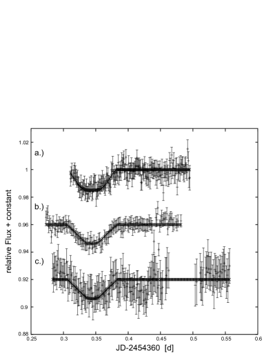
Figure 4: The TrES-2-transit from 2007 September 16 with three different telescopes: a.) $I$-band photometry from Jena b.) Wendelstein $R$-band observations c.) White light amateur observations

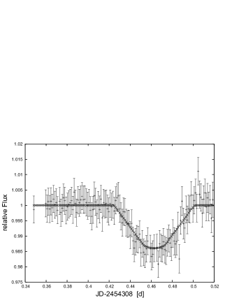
Figure 5: Wendelstein $R$-band photometry from 2007 July 26.

4 Determination of the midtransit time

Because the output of the IRAF task phot are magnitudes we convert our data to relative flux. We then calculate a weighted average of the pre-ingress and post-egress data and divided all data points by this value, in order to normalize the flux.
To determine the time of the center of the transit we fit an analytic light curve on the observed light curve. This analytic light curve was calculated with the stellar and planetary parameters given by Holman et al. (2007) and Sozzetti et al. (2007). To get the best fit we compare the analytic light curve with the observed light curve until the $\chi^{2}$ is minimal. The best fits of the analytic light curve to our observed data are shown as crosses in Fig. 2, 3, 4 and 5. With the help of the $\chi^{2}$-test we could determine the time of the midtransit even in the case of partial transits. We summarize the observed midtransit times in Table 2 marked with ”This work”. We give the 1-$\sigma$ error bars.

5 Ephemeris

Table 3: $UBVRI$ photometry of two Landolt standard stars and four secondary standard stars (from Galadí-Enríquez et al. 2000)

star	$\alpha_{2000}$	$\delta_{2000}$	$V$		$B\,-\,V$		$U\,-\,B$		$V\,-\,R$		$V\,-\,I$
SA 44 28${}^{a}$	00 29 04.00	+30 23 12.0	11.329 $\pm$	0.002	0.726 $\pm$	0.001	0.200 $\pm$	0.004	0.394 $\pm$	0.001	0.764 $\pm$	0.002
SA 44 113${}^{a}$	00 29 38.00	+30 23 18.0	11.713 $\pm$	0.006	1.206 $\pm$	0.002	0.996 $\pm$	0.019	0.667 $\pm$	0.003	1.229 $\pm$	0.005
8${}^{b}$	00 29 06.45	+30 25 29.6	14.539 $\pm$	0.006	0.765 $\pm$	0.005	0.276 $\pm$	0.006	0.426 $\pm$	0.004	0.809 $\pm$	0.007
9${}^{b}$	00 29 07.88	+30 18 07.1	13.099 $\pm$	0.007	0.609 $\pm$	0.003	-0.080 $\pm$	0.026	0.355 $\pm$	0.006	0.712 $\pm$	0.004
22${}^{b}$	00 29 20.55	+30 26 08.0	10.187 $\pm$	0.003	1.118 $\pm$	0.004	0.971 $\pm$	0.023	0.583 $\pm$	0.009	1.102 $\pm$	0.005
29${}^{b}$	00 29 33.25	+30 24 05.6	13.563 $\pm$	0.008	0.633 $\pm$	0.006	-0.043 $\pm$	0.021	0.348 $\pm$	0.006	0.666 $\pm$	0.005

${}^{a}$ Landolt (1983)

${}^{b}$ Numbers of standard stars in field #1 defined by Galadí-Enríquez et al. (2000)

In addition to the transits observed by us we could find 34 transit times from 2006-2008 in the literature. The altogether 44 transits are summarized in Table 2. We used the ephemeris of Holman et al. (2007) to compute ”observed minus calculated” (O-C) residuals for all 44 transit times. Fig. 6 shows the differences between the observed and predicted times of the center of the transit, as a function of epoch. The dashed line represents the ephemeris given by Holman et al. (2007). We found a negative trend in this (O-C)-diagram. Thus, we refine the ephemeris using the linear function for the heliocentric Julian date of midtransit (Eq. 4) where epoch $E$ is an integer and $T_{0}$ the midtransit to epoch 0.

$$T_{\mathrm{c}}=T_{0}+P\cdot E$$ (4)

For an exact determination of the ephemeris we plotted the midtransit times over the epoch and did a linear $\chi^{2}$-fit. We got the best $\chi^{2}$ with

$T_{0}(\mathrm{HJD})\,=\,(2453957.63492\pm 0.00013)\,\mathrm{d}$

and an orbital period of

$P\,=\,(2.470614\,\pm\,0.000001)\,\mathrm{d}$.

Our values for the $T_{0}$ and the period are different by 11.2 and 0.6 s, respectively, compared to the ones from Holman et al. (2007). The resulting ephemeris which represents our measurements best is

$$T_{\mathrm{c}}\mathrm{(HJD)}\,=\,(2453957.63492\,+\,E\cdot 2.470614)\,d$$ (5)

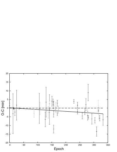
Figure 6: Transit timing residuals for TrES-2. The gray data points correspond to the measurements from the University Observatory Jena. The dashed line shows the ephemeris given by Holman et al. (2007). The best-fitting line (solid line) is plotted, representing the updated ephemeris given in equation 5.

6 Absolute photometry

To derive absolute photometric $V$, $R$ and $I$ magnitudes we observed the TrES-2 parent star on 2008 July 28, a photometric night. In order to perform the transformation to the standard system we observed standard star field #1 defined by Galadí-Enríquez et al. (2000) which is located around the two Landolt standard stars SA 44 28 and SA 44 113 (Landolt 1983). Altogether we took four images of the standard star field at different airmasses and a sequence of 32 TrES-2 parent star images in each filter. We measured the instrumental magnitudes of 6 standard stars - the two Landolt stars and four secondary standard stars ($UBVRI$ photometry given in Table 3, indentification chart shown in Fig. 7) - in each frame and calculated the zero point correction $c$ and the first order extinction coefficient $k$. The results for each filter are shown in Table 4.
During the analysis it turned out, that there is a faint object near the TrES-2 host star. We chose a larger aperture for the absolute photometry than for differential photometry (10 pixels instead of 5 pixels) to include this faint star in our measurements. With the help of the flux ratio of the two stars we could calculate the individual brightnesses. We finally derive the Bessell $V$, $R$ and $I$ magnitudes of the TrES-2 parent star obtained from the average of all 32 individual measurements. The errors given correspond to the standard deviation of these measurements:

$V\,=\,11.40\,\pm\,0.02$ mag

$R\,=\,11.08\,\pm\,0.02$ mag

$I\,=\,10.86\,\pm\,0.05$ mag

Our value for the $V$, $R$ and $I$ magnitudes are in good agreement with the ones published by O’Donavan et al. 2006 and Droege et al. 2006.

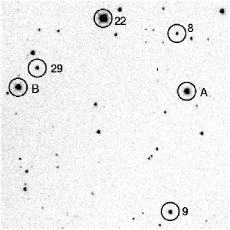
Figure 7: A 9.4${}^{\prime}\,\times$ 9.4${}^{\prime}$ 60 s $I$-band CTK-image section of standard star field #1 defined by Galadí-Enríquez et al. (2000). The circles marks the used standard stars. For a definition of the labels see Table 3. The two Landold stars SA 44 28 and SA 44 113 are labelled with ”A” and ”B”, respectively. North is up; east is to the left.

Table 4: zero point correction $c$ (normalized to 1 s exposure time) and first order extinction coefficient $k$ for each filter

Filter	$c$		$k$
$V$	18.96 $\pm$	0.03	0.27 $\pm$	0.02
$R$	18.94 $\pm$	0.02	0.21 $\pm$	0.02
$I$	18.42 $\pm$	0.02	0.16 $\pm$	0.01

7 The second dip

7.1 Detection of a second dip

In our first observation of a transit of TrES-2 (see Fig. 2 a.) the light curve shows an interesting behavior in the last part of the observations. After the transit is completed, the flux again decreases for a short time (about 30 min). The depth of this event amounts to 0.8 %, which is about half the depth of the transit. To check whether the dip is a real, reproducible event and no measuring error, we scheduled TrES-2 for our regular monitoring program. An indication of the existence of the dip is published by O’Donovan et al. (2006) in a TELAST $R$-band light curve in their Fig. 1, where one can clearly recognize a brightness drop.
On 2007 May 3 we succeeded a second time to observe a complete transit of TrES-2 (shown in Fig 2 c.). Again the dip is clearly visible after the transit is finished.

7.2 Further observations

As shown in section 2 we observed ten different transits. We could detect the second dip only after our first two transit observations (Fig. 2 a. and c.). Detailed analysis of the midtime of the dip showed that the dip moved away from the center of the transit (see Table 5). However, this does not follow a linear relationship.

Table 5: Movement of the dip relative to the center of the transit

Date	Distance${}^{a}$ [h]	projected
		separation${}^{b}$ [$\mu$as]
2006 August 10	1.07	19
2007 March 13	1.28	23
2007 May 3	1.80	32

${}^{a}$ Time between center of the transit and center of the dip
${}^{b}$ calculated for published distance of the TrES-2 host star (Sozzetti et al. 2007) and semi major axis of TrES-2 (O’Donovan et al. 2006)