The $\Sigma-D$ Analysis of Recently Detected Radio Planetary Nebulae in the Magellanic Clouds

Abstract

Aims. To investigate and analyze the radio surface brightness to diameter ($\Sigma-D$) relation for recently detected, bright radio-continuum planetary nebulae (PNe) in the Magellanic Clouds (MC).

Methods. We apply a Monte Carlo analysis in order to account for sensitivity selection effects on measured $\Sigma-D$ relation slopes for bright radio PNe in the MCs.

Results. In the $\Sigma-D$ plane these radio MCs PNe are positioned among the brightest of the nearby Galactic PNe, and are close to the $D^{-2}$ sensitivity line of the MCs radio maps. The fitted Large Magellanic Cloud (LMC) data slope appears to be influenced with survey sensitivity. This suggests the MCs radio PN sample represents just the “tip of the iceberg” of the actual luminosity function. Specifically, our results imply that sensitivity selection tends to flatten the slope of the $\Sigma-D$ relation. Although MCs PNe appear to share the similar evolution properties as Galactic PNe, small number of data points prevented us to further constrain their evolution properties.

1 Introduction

1.1 Radio bright Magellanic Cloud planetary nebulae

Filipović et al. (2009) recently reported 15 radio-continuum PNe detected at the $3\sigma$ and above level from various radio Magellanic Clouds (MCs) surveys. Their detections are mainly based on positional coincidences with optically detected Planetary Nebulae (PNe) and optical spectroscopy (Payne et al., 2008a, b). Included are Large Magellanic Cloud (LMC) mosaics (Dickel et al., 2005) having sensitivities of $\sim$0.5 mJy beam^-1 at both 4.8 and 8.64 GHz with resolutions of 33 and 20″, respectively. The Small Magellanic Cloud (SMC) mosaics have 0.5 mJy beam^-1 sensitivities at 4.8 and 8.64 GHz with resolutions of 30 and 15″ (Dickel, 2009). To compare these sources with Galactic PNe, we use radio surface brightness ($\Sigma$) since this quantity is distance independent:

$$\Sigma[\mathrm{W}\mathrm{m^{-2}\leavevmode\nobreak\ Hz^{-1}\leavevmode\nobreak\ sr^{-1}}]=1.505\times 10^{-19}\frac{S[\mathrm{Jy}]}{\theta^{2}[\mathrm{{}^{\prime}}]},$$ (1)

where $S$ is the flux density and $\theta$, the angular diameter of the source. Theory predicts the existence of a linear relation between $\log\Sigma$ and $\log D$, with $D$ representing the diameter of the object (see Urosevic et al., 2007; Urošević et al., 2009, and references therein).

All of the detected radio PNe are unresolved, despite five of them being observed in “snap-shot” mode with the resolution of up to 1″and sensitivity of $\sim 0.1\leavevmode\nobreak\ \mathrm{mJy\leavevmode\nobreak\ beam^{-1}}$ (for details see Filipović et al., 2009). The optical diameters are available for some 10 out of 15 (see Table 1 in Filipović et al., 2009). The MCs PNe data at 4.8 GHz are plotted in Fig. 1 with respective LMC map $3\sigma$ sensitivity line at $1.5\leavevmode\nobreak\ \mathrm{mJy\leavevmode\nobreak\ beam^{-1}}$ (hereafter referred to as sensitivity line). Five LMC PNe are above the sensitivity line and one is below (“snap-shot” mode). Five PNe with estimated upper flux density limit of $1.5\leavevmode\nobreak\ \mathrm{mJy\leavevmode\nobreak\ beam^{-1}}$ are plotted on the sensitivity line and the remaining one without optical diameter is not plotted. Four SMC PNe are plotted on the SMC map resolution limit of 30″. We use the PNe sample of Galactic PNe with reliable individual distances from Stanghellini, Shaw, & Villaver 2008; hereafter  SSV, and divide them into two subsamples (nearby PNe with distances smaller than 1 kpc and those with distances larger than 1 kpc). Urošević et al. (2009), in an extensive analysis of the empirical $\Sigma-D$ relation for PNe, argued that the SSV sample of nearby PNe is least influenced by selection effects. For comparison, we plot two radio PNe from the Sagittarius dwarf galaxy (Dudziak et al., 2000), also representative of extragalactic radio PNe. An arrow in Fig. 1 represents the $D^{-2}$ direction in which unresolved objects should move if their diameters were known.

Inspection of Fig. 1 reveal that the detected radio-continuum MCs PNe are very close to their sensitivity lines and they are as bright as the brightest Galactic PNe. When compared with Galactic PNe it appears that current data set is only the very peak of the actual MCs PNe luminosity function. In this paper, using $\chi^{2}$ analysis and Monte Carlo generated data samples, we investigate the sensitivity related selection effects on the $\Sigma-D$ properties of these objects and compare them with the properties of Galactic PNe.

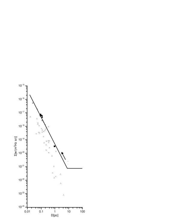
Figure 1: A plot of 4.8 GHz PNe from the LMC, SMC and Sagittarius Dwarf Galaxy. The solid line represents the LMC map sensitivity ($3\sigma$) at 1.5 mJy beam^-1. The LMC radio PNe with known optical diameters are represented with filled circles (above the sensitivity line, 5 PNe) and vertical dashes (sensitivity line is the upper flux density limit, 5 PNe). One LMC PN observed in ”snap-shot” mode is represented with filled square. The SMC radio PNe without known optical diameters are represented by horizontal dashes and asterisks are two Sagittarius Dwarf PNe. Open triangles represents Galactic SSV PNe with distances greater than 1 kpc while diagonal crosses are those with distances less than 1 kpc. Note that the arrow represents the direction in which MCs radio PNe should move on the graph, if their diameters were known.

1.2 Radio planetary nebulae sample selection effects - a brief history

As a convenient platform for distance determination, the $\Sigma-D$ relation has a $\sim$50 year long history of exploitation for supernova remnants (SNRs). The study of the relation for these very luminous radio synchrotron sources began with the work of Shklovskii (1960), while the first empirical $\Sigma-D$ relation was presented by Poveda & Woltjer (1968). Decades of analysis resulted in a good understanding of the $\Sigma-D$ relation for SNRs and various data sample selection effects that influence that relation.

The previous analysis of PNe radio data samples (e.g. Phillips, 2002, and references therein) were mainly focused on radius vs radio brightness temperature ($R-T_{\mathrm{b}}$) empirical relations. These were sparse in the consideration of data selection effects. Recent works by Urosevic et al. (2007); Urošević et al. (2009) use a SNR formalism in the analysis of PNe data along with a discussion of these selection effects. Although they note that all PN samples suffer from selection effects caused by limitations in survey sensitivity and resolution, the nearby SSV sample, having a $\Sigma-D$ slope of  $\beta=-2.61\pm 0.21$, is least influenced by these effects.

2 Analysis

2.1 Planetary nebulae data sample sets

Samples for Monte Carlo simulations are made using sources from Table 1 in Filipović et al. (2009) that have a known optical diameter (LMC sources only) and are above the map sensitivity line for a given frequency. This includes 5 PNe at both frequencies (8.64  and 4.8 GHz) though not necessarily the same ones. Using adopted distances to the LMC of 50 kpc and to the SMC of 60 kpc (Alves, 2004; Hilditch et al., 2005), the smallest sources in the selected samples have a mean geometrical diameter of 0.09 pc at both frequencies. The largest source has a mean geometrical diameter of 0.12 pc at 4.8 GHz and 0.15 pc at 8.64 GHz. Surface brightness ranges from ${2.67}\times 10^{-18}$ to $8.65\times 10^{-18}$ Wm^-2 Hz^-1 sr^-1 at 8.64 GHz and from ${4.70}\times 10^{-18}$ to $7.90\times 10^{-18}$ Wm^-2 Hz^-1 sr^-1 at 4.8 GHz. For the LMC maps, the 4.8 GHz sensitivity line is at $\Sigma={7.46}\times 10^{-22}$ Wm^-2 Hz^-1 sr^-1 with a $D^{-2}$ break at $D=8.00$ pc and a 8.64 GHz sensitivity line at $\Sigma={2.03}\times 10^{-21}$ and $D=4.85$ pc, respectively.

The relative flux density errors at both frequencies of the LMC maps are $<$10% (Filipović et al., 2009) and they are approximately the size of the symbols shown in Fig. 1. If we assume that the optical diameters have no significant errors and that the absolute flux density error equals the flux density standard deviation $\sigma_{\mathrm{S}}$, according to error propagation theory it follows from Eq. 1. that the standard deviation for $\log\Sigma$ ($\sigma_{\mathrm{log\Sigma}}$) is $0.434\leavevmode\nobreak\ \Delta S/S$. This gives $\sigma_{\mathrm{log\Sigma}}\approx 0.05$.

The resulting parameters of the $\log\Sigma=a+\beta*\log D$ fits are given in Table 1 for each frequency. The parameters $a$ and $\beta$, their standard uncertainties $\Delta a$ and $\Delta\beta$, the linear correlation coefficient $r$, the fit quality $r^{2}$, the probability $Q$ of obtaining larger WSSR (weighted sum of square residuals) and a ratio of WSSR to the number of degrees of freedom (ndof) are given in this table. A value of $0.1\gtrsim Q\gtrsim 0.001$ is expected for a statistically acceptable fit (the case when errors of the dependent variable have a non-Gaussian distribution), if the data is were well approximated by the model. This should apply for fits presented in this paper since we have transformed flux errors to $\log\Sigma$ errors. When introduced in the least squares fitting procedure, our values of $Q$ implies a statistically acceptable fit.

Although the fits are statistically believable the resulting $\beta$ at 4.8 GHz substantially differs from $\beta$ at 8.64 GHz, likely in debt to a small number of data points. Sampling only the peak of the luminosity function and with the majority of the sample likely hidden below the sensitivity line, the resulting values for $\beta$ should not be taken seriously. Comparing the LMC radio PN sample and the sample of a nearby Galactic PNe, we made an attempt to access a more meaningful $\Sigma-D$ slope using Monte Carlo simulations as described below.

Table 1: Fit parameters of the LMC data sample.

Frequency	$a$	$\Delta a$	$\beta$	$\Delta\beta$	$r$	$r^{2}$[%]	$Q$	$\mathrm{\frac{WSSR}{ndof}}$
8.64 GHz	–19.7	0.3	–2.6	0.4	–0.94	88.36	$5.02\times 10^{-2}$	2.60
4.80 GHz	–18.1	0.5	–0.9	0.5	–0.64	40.96	$9.96\times 10^{-2}$	2.08

2.2 Monte Carlo simulations

We performed Monte Carlo simulations similar to those described by Urošević et al. (2005). The results of their simulations (with 21 data points above the sensitivity line) showed that slopes steeper than $-2$ are under influence of sensitivity related selection effects. First, we determined the empirical $\log\Sigma$ standard deviation from the best fit line, assuming $\log D$ as the independent variable. We then selected an interval in $\log D$ five times as long as that of the real data. This interval is then sprinkled with random points of the same $\log D$ density as that of the real data.

The simulated points, that lie on the log D axis, are then projected onto a series of lines at different slopes (in steps of 0.1 from –3.5 to –1.5). Each of these lines passes through the extreme upper left hand end of the best fit line to the real data. We also added Gaussian noise in $\log\Sigma$, which is related to the scatter of the real data by a parameter called “scatter”. A scatter of 1 corresponds to the same standard deviation as that of the real data.

An appropriate sensitivity cutoff is applied to the simulated data points, selecting points above the sensitivity line. This is done 100 times for each simulated slope and a least squares best fit line is generated for artificial samples that have five or more selected data points. The number of such samples is given in the last column of Tables 2 and 3.

In Tables 2 and 3, the first column lists the value of the simulated slope, while the mean and standard deviation of the best fit slopes for the generated samples are given in second and third column, respectively. The fourth and fifth column gives the mean and standard deviation of the best fit slopes for sensitivity selected generated samples, respectively. In Fig. 2 we present one of our Monte Carlo generated samples at 8.64 GHz for a scatter of 1 and the simulated slope –2.7.

Figure 2: The Monte Carlo generated sample at 8.64 GHz for a scatter of 2 and simulated slope of –2.7. The LMC data points (asterisks) are plotted along with the sensitivity (thick solid) line; artificially generated points are plotted above (filled circles) and below (open circles) this line. The selection of points above the sensitivity line give a fit with a flatter slope (thin solid line) than the slope of a fit using all simulated points (dotted line).

Table 2: Monte Carlo simulation results at 4.8 GHz.

The slope	Mean	Standard	Mean	Standard	No. of
that is	simulated	deviation	slope	deviation	generated
simulated	slope	of mean	after	of slope	samples
		simulated	selection	after	that was
		slope		selection	fitted
scatter=1.0
–1.500000	–1.492251	0.068066	–1.514832	0.064286	100
–1.600000	–1.598043	0.068590	–1.623227	0.062590	100
–1.700000	–1.699330	0.065987	–1.728391	0.064682	100
–1.800000	–1.801370	0.061776	–1.827670	0.062875	100
–1.900000	–1.904920	0.065998	–1.939695	0.063711	100
–2.000000	–2.003822	0.057447	–2.001172	0.059317	100
–2.100000	–2.099951	0.065622	–2.041389	0.062283	100
–2.200000	–2.195110	0.063386	–2.070956	0.086876	99
–2.300000	–2.297590	0.064135	–2.074784	0.130676	82
–2.400000	–2.398137	0.070116	–2.110495	0.211172	59
–2.500000	–2.501291	0.065666	–2.180770	0.426777	40
–2.600000	–2.594927	0.068783	–2.222386	0.527765	23
–2.700000	–2.700259	0.065226	–2.347649	0.527067	11
–2.800000	–2.801124	0.071673	–2.339542	0.345267	11
–2.900000	–2.892171	0.061980	–2.325770	0.384151	9
–3.000000	–2.995751	0.067793	–2.814787	0.608717	4
–3.100000	–3.093523	0.066956	–2.789218	0.225177	3
–3.200000	–3.093523	0.131417	–	–	0
–3.300000	–3.304876	0.071690	–2.841456	0.077769	3
–3.400000	–3.304876	0.126657	–2.841456	–	1
–3.500000	–3.502017	0.064626	–2.471982	0.471662	3
scatter=2.0
–1.500000	–1.494408	0.129362	–1.582530	0.129317	100
–1.600000	–1.582302	0.137065	–1.684048	0.127792	100
–1.700000	–1.710318	0.142266	–1.786533	0.126412	100
–1.800000	–1.803957	0.135674	–1.896290	0.127258	100
–1.900000	–1.908844	0.128375	–1.957930	0.123818	100
–2.000000	–1.977503	0.128244	–1.979623	0.101482	100
–2.100000	–2.126453	0.124008	–2.047942	0.106982	100
–2.200000	–2.218740	0.132994	–2.069085	0.121897	99
–2.300000	–2.301067	0.118757	–2.100132	0.180063	96
–2.400000	–2.422463	0.156185	–2.121199	0.220895	85
–2.500000	–2.489904	0.122634	–2.137602	0.234918	73
–2.600000	–2.596131	0.130540	–2.133221	0.314863	54
–2.700000	–2.715585	0.105664	–2.166716	0.624909	38
–2.800000	–2.784944	0.118933	–2.127692	0.398607	30
–2.900000	–2.922056	0.123773	–2.334104	0.607681	16
–3.000000	–3.007808	0.115488	–2.198724	1.185409	20
–3.100000	–3.090180	0.137786	–2.386109	0.311125	10
–3.200000	–3.181103	0.140162	–2.454902	1.599802	6
–3.300000	–3.319871	0.139671	–1.996534	0.496468	9
–3.400000	–3.389912	0.124211	–2.349205	0.254864	4
–3.500000	–3.389912	0.168488	–2.349205	–	1

Table 3: Monte Carlo simulation results at 8.64 GHz.

The slope	Mean	Standard	Mean	Standard	No. of
that is	simulated	deviation	slope	deviation	generated
simulated	slope	of mean	after	of slope	samples
		simulated	selection	after	that was
		slope		selection	fitted
scatter=1.0
–1.500000	–1.503405	0.052604	–1.503405	0.052604	100
–1.600000	–1.600591	0.042812	–1.601002	0.042035	100
–1.700000	–1.698601	0.037607	–1.698601	0.037607	100
–1.800000	–1.792767	0.040580	–1.792767	0.040580	100
–1.900000	–1.893138	0.043315	–1.893138	0.043315	100
–2.000000	–1.995468	0.045243	–1.994920	0.045646	100
–2.100000	–2.102842	0.042350	–2.088784	0.045885	100
–2.200000	–2.193731	0.042313	–2.144698	0.044331	100
–2.300000	–2.298443	0.045962	–2.187980	0.069080	100
–2.400000	–2.401427	0.048780	–2.269207	0.107564	100
–2.500000	–2.501493	0.043743	–2.318480	0.162147	98
–2.600000	–2.601538	0.043349	–2.425642	0.195200	98
–2.700000	–2.699132	0.040760	–2.449996	0.249949	81
–2.800000	–2.803434	0.040787	–2.553920	0.368122	62
–2.900000	–2.895824	0.040305	–2.556149	0.549145	56
–3.000000	–3.000702	0.041717	–2.694128	0.306140	49
–3.100000	–3.100702	0.039240	–2.703438	0.557734	40
–3.200000	–3.199087	0.044836	–2.836055	0.529287	28
–3.300000	–3.303262	0.042204	–2.874302	0.325416	15
–3.400000	–3.394428	0.044995	–2.775834	0.499802	18
–3.500000	–3.495130	0.043181	–2.928748	0.433336	14
scatter=2.0
–1.500000	–1.499001	0.073477	–1.506813	0.071878	100
–1.600000	–1.595906	0.091924	–1.609181	0.091654	100
–1.700000	–1.706313	0.079195	–1.720427	0.077824	100
–1.800000	–1.801306	0.077013	–1.818025	0.079255	100
–1.900000	–1.892254	0.092443	–1.903992	0.083989	100
–2.000000	–2.002529	0.093860	–2.007141	0.092602	100
–2.100000	–2.094921	0.087675	–2.065955	0.079765	100
–2.200000	–2.196983	0.097031	–2.109052	0.089702	100
–2.300000	–2.278865	0.094011	–2.135513	0.085328	100
–2.400000	–2.403615	0.089715	–2.205754	0.141621	100
–2.500000	–2.478826	0.080478	–2.194225	0.191552	98
–2.600000	–2.593142	0.095069	–2.264253	0.276645	89
–2.700000	–2.709181	0.091667	–2.402365	0.329761	85
–2.800000	–2.799243	0.076143	–2.297942	0.374669	67
–2.900000	–2.901775	0.080564	–2.406221	0.411391	61
–3.000000	–2.999507	0.086134	–2.591900	0.528155	41
–3.100000	–3.083982	0.090140	–2.527112	0.497492	31
–3.200000	–3.187697	0.081336	–2.453453	0.617842	29
–3.300000	–3.303730	0.089221	–2.681570	1.138125	32
–3.400000	–3.392252	0.084091	–2.712006	0.649541	20
–3.500000	–3.501420	0.078870	–2.584415	0.885438	21

3 Discussion and conclusions

From tables 2 and 3, it is evident that the sensitivity cutoff tends to flatten the intrinsic (simulated) slopes less than –2 (the most likely case for the real data). At 4.8 GHz, a slope of $-0.9\pm 0.5$ (shallower than the sensitivity line) is not influenced with sensitivity related selection effects. From the other side, this slope does not have any physical interpretation and is only the consequence of scatter in the $\Sigma-D$ plane. The 8.64 GHz slope of $-2.6\pm 0.4$ appears to correspond to somewhat steeper selection free slopes but due to a large error could have any value smaller than –2.3. This is within the range of the SSV slope at 4.8 GHz. With current LMC data samples it is not possible to constrain the lower limit due to a smaller number of selected points for steeper slopes. The value of a mean slope after selection at 8.64 GHz starts to oscillate for the slopes $\lesssim-2.4$ (the standard deviation of slope after selection exceeds the interval between two successive simulated slopes). Table 2 is given here rather for completeness, but nevertheless, shows that for the samples with small number of data points and a slope larger than –2 it is not possible to extract any meaningful information with this kind of simulations.

With these recently confirmed MCs radio PNe being amongst brightest Galactic PNe in the $\Sigma-D$ plane and given their proximity to the sensitivity line, it is likely they represent only the peak of the actual MCs PNe luminosity function, which is probably the ”bright-end” extension of the Galactic PNe luminosity function (for a more detailed discussion on the nature of these MCs PNe see Filipović et al., 2009). The results of our LMC Monte Carlo simulations suggest that current sparse data samples cannot give meaningful $\Sigma-D$ slope. However, they confirmed that the corresponding apparent $\Sigma-D$ slope flattens toward $\beta\approx-2$ because of the sensitivity related selection effects..

This should be kept in mind as a serious measure of caution in forthcoming studies of extragalactic PN samples. Future high sensitivity images of the MCs will surely provide even better and more complete radio samples of PN population and enable more robust constraining of PN evolution parameters.