The Subleading Term of the Strong Coupling Expansion of the Heavy-Quark Potential in a $\mathcal{N}=4$ Super Yang-Mills Vacuum

Abstract:

Applying the AdS/CFT correspondence, the expansion of the heavy-quark potential of ${\cal N}=4$ supersymmetric Yang-Mills theory at large $N_{c}$ is carried out to the sub-leading term in the large ’t Hooft coupling at zero temperature. The strong coupling corresponds to the semi-classical expansion of the string-sigma model, the gravity dual of the Wilson loop operator, with the sub-leading term expressed in terms of functional determinants of fluctuations. The singularities of these determinants are examined and their contributions are evaluated numerically.

1 Introduction

AdS/CFT duality [1, 2, 3, 4] remains an active field of research. Motivated by the isomorphism between the isometry group of AdS₅ and the conformal group in four dimensions, it was conjectured by Maldacena that a string theory in AdS${}_{5}\times S^{5}$ corresponds to a four dimensional conformal field theory on the boundary. A prominent implication of the conjecture is the correspondence between the type IIB superstring theory formulated on AdS${}_{5}\times S^{5}$ and $\mathcal{N}=4$ supersymmetric Yang-Mills theory (SYM) with the isometry group $O(6)$ of $S^{5}$ dual to the R-symmetriy group $SU(4)$ of SYM. In particular, the supergravity limit of the string theory corresponds to the leading behavior of SYM at large $N_{c}$ and large ’t Hooft coupling

$$\lambda\equiv g_{\rm YM}^{2}N_{c}={\frac{L^{4}}{\alpha^{\prime 2}}}.$$ (1)

with $L$ the AdS radius and $\alpha^{\prime}$ the reciprocal of the string tension. This relation thereby opens a new avenue to explore the strong coupling properties of SYM and sheds new lights on strongly coupled QGP created in RHIC in spite of the difference between SYM and QCD. Among notable successes on the RHIC phenomenology are the equation of state [5], the viscosity ratio[6] and jet quenching parameters [7] as well as the energy loss[8].

The heavy quark potential (the potential energy between a heavy quark and its anti-particle) of QCD is an important quantity that probes the confinement mechanism in the hadronic phase and the meson melting in the plasma phase. It is extracted from the expectation of a Wilson loop operator, which can be measured on a lattice. In the case of $\mathcal{N}=4$ SYM, the AdS/CFT duality relates the Wilson loop expectation value to the path integral of the string-sigma action developed in Ref.[9] for the worldsheet in the AdS${}_{5}\times S^{5}$ bulk spanned by the loop on the boundary. To the leading order of strong coupling, the path integral is given by its classical limit, which is the minimum area of the world sheet. From the Wilson loop of a pair of parallel lines, Maldacena extracted the potential function in $\mathcal{N}=4$ SYM at zero temperature[10],

$$V(r)=-\frac{4\pi^{2}}{\Gamma^{4}\left(\frac{1}{4}\right)}\frac{\sqrt{\lambda}}{r}\simeq-0.2285\frac{\sqrt{\lambda}}{r}$$ (2)

with $r$ the distance between the quark and the antiquark. Introducing a black hole in AdS bulk, the potential at nonzero temperature as well as that for moving quarks have been obtained by a number of authors[11][12]. The field theoretic aspects of the potential (2) and its finite temperature counterpart as well as their implications on RHIC physics were discussed in Ref.[13][14][12]. As was pointed out in Ref.[10], the ”heavy quarks” underlying the Wilson loop (2) in ${\cal N}=4$ SYM are actually heavy W bosons resulted in a Higgs mechanism, which implement the fundamental representation of $SU(N_{c})$. Since the function (2) measures the force between two static fundamental color objects, we shall borrow the terminology of QCD by naming it the heavy quark potential throughout this paper.

The strong coupling expansion of the SYM Wilson loop corresponds to the semi-classical expansion of the string-sigma action and reads

$$V(r)=-\frac{4\pi^{2}}{\Gamma^{4}\left(\frac{1}{4}\right)}\frac{\sqrt{\lambda}}{r}\Big{[}1+\frac{\kappa}{\sqrt{\lambda}}+O\left(\frac{1}{\lambda}\right)\Big{]}$$ (3)

for the heavy quark potential. Computing the coefficient $\kappa$ is the main subject of the present paper. $\kappa$ comes from the one loop effective action of the world sheet fluctuations around its minimum area. This effective action has been obtained explicitly for some simple Wilson loops including parallel lines[15] [16] and is expressed in terms of functional determinants. Evaluating these determinants, we end up with the numerical value of $\kappa$,

$$\kappa\simeq-1.33460.$$ (4)

The classical solution of the string-sigma model and the one loop effective action underlying $\kappa$ is briefly reviewed in the next section. There we also outline our strategy of computation, which is along the line suggested in [16]. We parametrize the string world sheet of the single Wilson line or parallel lines by conformal coordinates. Then a scaling transformation is made that leaves the measure of the spectral problem of the functional determinants trivial. Instead of solving the eigenvalue problem of the operators underlying the determinants, we use the method employed in [17], which amounts to solve a set of ordinary differential equations. Unlike the straight Wilson line and the circular Wilson loop dealt with in [17], some of differential equations for the parallel lines are not analytically tractable. The presence of various singularities makes numerical works highly nontrivial. It is critical to isolate the singularities analytically in order to obtain a robust numerical result. So we did and the procedure is described in sections 3 and 4. The finite terms of the scaling transformation of the determinants involved are examined in section 5 and we find them adding up to zero. In section 6, we discuss our results along with few open questions. Some technical details are explained in appendices. Throughout the paper, we shall work with Euclidean signature with the AdS radius $L$ set to one.

2 The one-loop effective action

Let us begin with a brief review of the classical limit that leads to the leading order potential (2). The string-sigma action in this limit reduces to the Nambu-Goto action

$$S_{\rm NG}=\frac{1}{2\pi\alpha^{\prime}}\int d^{2}\sigma\sqrt{g},$$ (5)

with $g$ the determinant of the induced metric on the string world sheet embedded in the target space, i.e.

$$g_{\alpha\beta}=G_{\mu\nu}\frac{\partial X^{\mu}}{\partial\sigma^{\alpha}}\frac{\partial X^{\nu}}{\partial\sigma^{\beta}}$$ (6)

where $X^{\mu}$ and $G_{\mu\nu}$ are the target space coordinates and the metric, and $\sigma^{\alpha}$ with ($\alpha=0,1$) parametrize the world sheet. The target space here is AdS${}_{5}\times S^{5}$, whose metric may be written as

$$ds^{2}=\frac{1}{z^{2}}(dt^{2}+d\vec{x}^{2}+dz^{2})+d\Omega_{5}^{2}$$ (7)

with $d\Omega_{5}$ the element of the solid angle of S⁵. The physical 3-brane resides on the AdS boundary $z=0$. The string world sheets considered in this paper are all projected onto a point of S⁵ in the classical limit.

The Wilson loop of a static heavy quark, denoted by ${\cal C}_{1}$, is a straight line winding up the Euclidean time periodically at the AdS boundary. The corresponding world sheet in the AdS bulk can be parametrized by $t$ and $z$ with $\vec{x}$ constant and extends all the way to AdS horizon, $z\to\infty$. The induced metric is that of AdS₂, given by

$$ds^{2}[{\cal C}_{1}]=\frac{1}{z^{2}}(dt^{2}+dz^{2})$$ (8)

with the scalar curvature

$$R=-2.$$ (9)

Substituting the metric (8) into (5), we find the self-energy of the heavy quark

$$E[{\cal C}_{1}]=\frac{1}{T}S_{\rm NG}[{\cal C}_{1}]=\frac{1}{2\pi\alpha^{\prime}}\int_{\delta}^{\infty}\frac{dz}{z^{2}}.$$ (10)

with $T\to\infty$ the time period. Notice that we have pulled the physical brane slightly off the boundary to the radial coordinate $z=\delta$, as a regularization of the divergence pertaining the lower limit of the integral (10).

The total energy of a pair of a heavy quark and a heavy antiquark separated by a distance $r$, can be extracted from the Wilson loop consisting of two parallel lines each winding up the Euclidean time at the boundary. This Wilson loop will be denoted by ${\cal C}_{2}$ and the world sheet in the bulk can be parametrized by $t$ and $z$ with $x^{1}=\xi(z)$ and $x^{2},x^{3}={\rm const.}$. The function $\xi(z)$ is determined by substituting the induced metric

$$ds^{2}[{\cal C}_{2}]=\frac{1}{z^{2}}\{dt^{2}+\Big{[}\left(\frac{d\xi}{dz}\right)^{2}+1\Big{]}dz^{2}\},$$ (11)

into the action (5) and minimizing it. We have

$$\xi=\pm\int_{z}^{z_{0}}dz^{\prime}\frac{z^{\prime 2}}{\sqrt{z_{0}^{4}-z^{\prime 4}}}.$$ (12)

The maximum bulk extension of the world sheet, $z_{0}$, is determined by the distance $r$ between the two lines at the boundary and we find that

$$z_{0}=\frac{\Gamma^{2}\left(\frac{1}{4}\right)}{(2\pi)^{\frac{3}{2}}}r$$ (13)

Substituting (12) into (11), we end up with the induced metric

$$ds^{2}[{\cal C}_{2}]=\frac{1}{z^{2}}\left(dt^{2}+\frac{z_{0}^{4}}{z_{0}^{4}-z^{4}}dz^{2}\right),$$ (14)

and the scalar curvature

$$R=-2\left(1+\frac{z^{4}}{z_{0}^{4}}\right)$$ (15)

The energy of the heavy quark pair is therefore given by,

$$E[{\cal C}_{2}]=\frac{1}{T}S_{\rm NG}[{\cal C}_{2}]=\frac{1}{\pi\alpha^{\prime}}z_{0}^{2}\int_{\delta}^{z_{0}}\frac{dz}{z^{2}\sqrt{z_{0}^{4}-z^{4}}},$$ (16)

where the same regularization is applied to the lower limit of the integral.

The heavy quark potential is obtained by subtracting from (16) the self energy of each quark(antiquark), i.e.

$$V=\lim_{\delta\to 0^{+}}(E[{\cal C}_{2}]-2E[{\cal C}_{1}])=\frac{1}{\pi\alpha^{\prime}}\Big{[}\int_{0}^{z_{0}}dz\left(\frac{z_{0}^{2}}{z^{2}\sqrt{z_{0}^{4}-z^{4}}}-\frac{1}{z^{2}}\right)-\frac{1}{z_{0}}\Big{]},$$ (17)

and is divergence free. Carrying out the integral and substituting in the relations (13), we derive (2).

The one loop effective action, $W$ is obtained by expanding the string-sigma action of Ref.[9] to the quadratic order of the fluctuating coordinates around the minimum area and carrying out the path integral[15][16]. We have

$$W[{\cal C}_{1}]=-\ln\Big{[}\frac{{\det}^{4}(-i\gamma^{\alpha}\nabla_{\alpha}+\tau_{3})}{{\det}^{\frac{3}{2}}(-\nabla^{2}+2){\det}^{\frac{5}{2}}(-\nabla^{2})}\Big{]},$$ (18)

for the static quark or antiquark and

$$W[{\cal C}_{2}]=-\ln\Big{[}\frac{{\rm det}^{4}(-i\gamma^{\alpha}\nabla_{\alpha}+\tau_{3})}{{\det}^{\frac{1}{2}}(-\nabla^{2}+4+R)\,{\det}(-\nabla^{2}+2)\,{\det}^{\frac{5}{2}}(-\nabla^{2})}\Big{]},$$ (19)

for the quark pair. The determinants in the denominators of (18) and (19) come from the fluctuations of three transverse coordinates of the AdS sector and five coordinates of $S^{5}$ with the Laplacian given by the metric (8) or (14). The determinants in the numerators come from the fermionic fluctuations, where we have introduced 2d gamma matrices, $\gamma_{0}=\gamma^{0}=\tau_{2}$, $\gamma_{1}=\gamma^{1}=\tau_{1}$ and $\gamma_{0}\gamma_{1}=-i\tau_{3}$ with $\tau_{1}$, $\tau_{2}$ and $\tau_{3}$ the three Pauli matrices. In terms of the zweibein of the world sheet, $e_{\alpha}^{j}$, we have $\gamma_{\alpha}\equiv e_{\alpha}^{j}\gamma_{j}$ with $j=0,1$ and the covariant derivative

$$\nabla_{\alpha}=\frac{\partial}{\partial\sigma^{\alpha}}+\frac{1}{8}[\gamma_{i},\gamma_{j}]\omega_{\alpha}^{ij}$$ (20)

with $\omega_{\alpha}^{ij}$ the spin connection corresponding to (8) or (14). The power ”4” comes from eight 2d Majorana fermions each of which contributes a power 1/2. The one loop correction to the heavy quark potential is then

$$\Delta V=\lim_{T\to\infty}\frac{1}{T}\lim_{\delta\to 0^{+}}(W[{\cal C}_{2}]-2W[{\cal C}_{1}]).$$ (21)

The effective action $W[{\cal C}_{1}]$ or $W[{\cal C}_{2}]$ suffers from the usual logarithmic UV divergence, which is proportional to the volume part of the Euler character

$$\int_{z>\delta}dtdz\sqrt{g}R$$ (22)

of each world sheet with the same coefficient of proportionality[16]. It follows from (8), (9), (14) and (15) that the integral (22) for the parallel lines is exactly twice of that for the single line in the limit $\delta\to 0$. We have indeed that

$$\int d^{2}\sigma\sqrt{g}R=T\int_{\delta}^{\infty}\frac{dz}{z^{2}}(-2)=-\frac{2T}{\delta}$$ (23)

for the single line and

$$\int d^{2}\sigma\sqrt{g}R=2T\int_{\delta}^{z_{0}}dz\frac{z_{0}^{2}}{\sqrt{z_{0}^{4}-z^{4}}}(-2)\left(1+\frac{z^{4}}{z_{0}^{4}}\right)=\left.\frac{4T}{z}\sqrt{1-\frac{z^{4}}{z_{0}}}\right|_{\delta}^{z_{0}}=-\frac{4T}{\delta}+O(\delta^{3}).$$ (24)

for the parallel lines. Therefore the UV divergence as well as the conformal anomaly cancel in the combination of (21) in the limit $\delta\to 0$. As a contrast, the volume integral $\int d^{2}\sigma\sqrt{g}$ of the parallel lines differs from twice of that of a straight line by a finite quantity in the same limit. The UV divergence associated to the volume integral cancels within each effective action of (18) and (19)[18]. Furthermore the limit $\delta\to 0^{+}$ of the UV finite term of (21) also exists as we shall see.

The world sheet of the parallel lines covers the coordinate patch $(t,z)$ twice, which gives rise to an artificial singularity of the Laplacian’s in (19) at $z=z_{0}$ and adds difficulties to the numerical works. To avoid the problem, we shall work with a conformal coordinate patch $(\tau,\sigma)$ that the world sheet (14) covers only once. This is also suggested in [16]. The new coordinates involve Jacobi elliptic functions [19][20]of modulo $k=\frac{1}{\sqrt{2}}$ and are defined by

$$z=z_{0}{\rm cn}\sigma\qquad t=\frac{z_{0}}{\sqrt{2}}\tau$$ (25)

In terms of the new coordinates, the metric (14) takes the form

$$ds^{2}[{\cal C}_{2}]=\frac{1}{2{\rm cn}^{2}\sigma}(d\tau^{2}+d\sigma^{2}),$$ (26)

and the scalar curvature (15) becomes

$$R=-2(1+{\rm cn}^{4}\sigma).$$ (27)

The nonzero component of the spin connection with cartesian indexes (0,1) referring to the coordinate differentials $d\tau$ and $d\sigma$ reads

$$\omega_{\tau}^{01}=-\omega_{\tau}^{10}=\frac{{\rm sn}\sigma{\rm dn}\sigma}{{\rm cn}\sigma}.$$ (28)

We shall use the the same time variable $\tau$ to describe the world sheet of the straight line and rescale the $z$ coordinate by $z=\frac{z_{0}}{\sqrt{2}}\zeta$, leaving the conformal structure of (8) intact, i.e.

$$ds^{2}[{\cal C}_{1}]=\frac{1}{\zeta^{2}}(d\tau^{2}+d\zeta^{2}).$$ (29)

The spin connection corresponding to (28) is given by $\omega_{\tau}^{01}=-\omega_{\tau}^{10}=-\frac{1}{\zeta}$. The range of each coordinate variable is $-\frac{{\cal T}}{2}\leq\tau\leq\frac{{\cal T}}{2}$, $-K\leq\sigma\leq K$ and $0\leq\zeta<\infty$ where ${\cal T}=\frac{\sqrt{2}}{z_{0}}T$ and $K$ is the complete elliptic integral of the first kind,

$$K=\frac{\Gamma^{2}\left(\frac{1}{4}\right)}{4\sqrt{\pi}}\simeq 1.8541.$$ (30)

The operators underlying the determinants of (18) are given explicitly by

$$\Delta_{0}[{\cal C}_{1}]\equiv-\nabla^{2}=-\zeta^{2}\left(\frac{\partial^{2}}{\partial\tau^{2}}+\frac{\partial^{2}}{\partial\zeta^{2}}\right)\equiv\zeta^{2}\hat{\Delta}_{0}[{\cal C}_{1}]$$ (31)

$$\Delta_{1}[{\cal C}_{1}]\equiv-\nabla^{2}+2=-\zeta^{2}\left(\frac{\partial^{2}}{\partial\tau^{2}}+\frac{\partial^{2}}{\partial\zeta^{2}}\right)+2\equiv\zeta^{2}\hat{\Delta}_{1}[{\cal C}_{1}]$$ (32)

and

$$D_{F}[{\cal C}_{1}]\equiv-i\gamma^{\alpha}\nabla_{\alpha}+\tau_{3}=-i\zeta\left(\frac{d}{d\zeta}-\frac{1}{2\zeta}\right)\tau_{1}-i\zeta\frac{\partial}{\partial\tau}\tau_{2}+\tau_{3}\equiv\zeta\hat{D}_{F}[{\cal C}_{1}].$$ (33)

Similarly, the explicit expressions of the operators underlying the determinants of (19) reads

$$\Delta_{0}[{\cal C}_{2}]\equiv-\nabla^{2}=-2{\rm cn}^{2}\sigma\left(\frac{\partial^{2}}{\partial\tau^{2}}+\frac{\partial^{2}}{\partial\sigma^{2}}\right)\equiv 2{\rm cn}^{2}\sigma\hat{\Delta}_{0}[{\cal C}_{2}],$$ (34)

$$\Delta_{1}[{\cal C}_{2}]\equiv-\nabla^{2}+2=-2{\rm cn}^{2}\sigma\left(\frac{\partial^{2}}{\partial\tau^{2}}+\frac{\partial^{2}}{\partial\sigma^{2}}\right)+2\equiv 2{\rm cn}^{2}\sigma\hat{\Delta}_{1}[{\cal C}_{2}],$$ (35)

$$\Delta_{2}[{\cal C}_{2}]\equiv-\nabla^{2}+4+R=-2{\rm cn}^{2}\sigma\left(\frac{\partial^{2}}{\partial\tau^{2}}+\frac{\partial^{2}}{\partial\sigma^{2}}\right)+2(1-{\rm cn}^{4}\sigma)\equiv 2{\rm cn}^{2}\sigma\hat{\Delta}_{2}[{\cal C}_{2}],$$ (36)

and

$$D_{F}[{\cal C}_{2}]\equiv-i\gamma^{\alpha}\nabla_{\alpha}+\tau_{3}=-i\sqrt{2}{\rm cn}\sigma\left(\frac{\partial}{\partial\sigma}+\frac{{\rm sn}\sigma{\rm dn}\sigma}{2{\rm cn}\sigma}\right)\tau_{1}-i\sqrt{2}{\rm cn}\sigma\frac{\partial}{\partial\tau}\tau_{2}+\tau_{3}\equiv{\rm cn}\sigma\hat{D}_{F}[{\cal C}_{2}].$$ (37)

The difference between the operators with hats and those without hats is the measure of the spectral problem defined by them. While the measure is trivial with respect to the operators with hats, changing the measure may introduce additional terms to the logarithm of each determinant and their contribution will be examined in section V. For this reason, the effective action is decomposed into two pieces, i.e. $W[{\cal C}_{1}]=W_{1}[{\cal C}_{1}]+W_{2}[{\cal C}_{1}]$ for the single Wilson line and $W[{\cal C}_{2}]=W_{1}[{\cal C}_{2}]+W_{2}[{\cal C}_{2}]$ for the parallel lines. We define

$$W_{1}[{\cal C}_{1}]=-\ln\frac{\det^{4}\hat{D}_{F}[{\cal C}_{1}]}{\det^{\frac{5}{2}}\hat{\Delta}_{0}[{\cal C}_{1}]\det^{\frac{3}{2}}\hat{\Delta}_{1}[{\cal C}_{1}]},$$ (38)

$$W_{2}[{\cal C}_{1}]=-4\ln\frac{|\det D_{F}[{\cal C}_{1}]|}{|\det\hat{D}_{F}[{\cal C}_{1}]|}+\frac{5}{2}\ln\frac{\Delta_{0}[{\cal C}_{1}]}{\hat{\Delta}_{0}[{\cal C}_{1}]}+\frac{3}{2}\ln\frac{\Delta_{1}[{\cal C}_{1}]}{\hat{\Delta}_{1}[{\cal C}_{1}]},$$ (39)

$$W_{1}[{\cal C}_{2}]=-\ln\frac{\det^{4}\hat{D}_{F}[{\cal C}_{2}]}{\det^{\frac{5}{2}}\hat{\Delta}_{0}[{\cal C}_{2}]\det\hat{\Delta}_{1}[{\cal C}_{2}]\det^{\frac{1}{2}}\hat{\Delta}_{2}[{\cal C}_{2}]},$$ (40)

and

$$W_{2}[{\cal C}_{2}]=-4\ln\frac{|\det D_{F}[{\cal C}_{2}]|}{|\det\hat{D}_{F}[{\cal C}_{2}]|}+\frac{5}{2}\ln\frac{\Delta_{0}[{\cal C}_{2}]}{\hat{\Delta}_{0}[{\cal C}_{2}]}+\ln\frac{\Delta_{1}[{\cal C}_{2}]}{\hat{\Delta}_{1}[{\cal C}_{2}]}+\frac{1}{2}\ln\frac{\Delta_{2}[{\cal C}_{2}]}{\hat{\Delta}_{2}[{\cal C}_{2}]},$$ (41)

Correspondingly, the coefficient $\kappa$ defined in (3) is given by $\kappa=\kappa_{1}+\kappa_{2}$ with

$$\kappa_{1}\equiv\frac{\Gamma^{2}\left(\frac{1}{4}\right)}{\sqrt{\pi}{\cal T}}\lim_{\delta\to 0^{+}}(W_{1}[{\cal C}_{2}]-2W_{1}[{\cal C}_{1}]),$$ (42)

and

$$\kappa_{2}\equiv\frac{\Gamma^{2}\left(\frac{1}{4}\right)}{\sqrt{\pi}{\cal T}}\lim_{\delta\to 0^{+}}(W_{2}[{\cal C}_{2}]-2W_{2}[{\cal C}_{1}]),$$ (43)

where we have used the relation between $T$ and ${\cal T}$ and converted $z_{0}$ to $r$ via (13).

Making a Fourier transformation of the time variable $\tau$, each functional determinant of (18) and (19) is factorized as an infinite product of its Fourier components with each Fourier component obtained by replacing the time derivative $\frac{\partial}{\partial\tau}$ in $\hat{\Delta}$’s of (31)-(37) by $-i\omega$ with $\omega$ a frequency variable. Substituting the Fourier product of (18) and that of (19) into (42), we find that

$$\kappa_{1}=\frac{\Gamma^{2}\left(\frac{1}{4}\right)}{\sqrt{\pi}}\int_{-\infty}^{\infty}\frac{d\omega}{2\pi}\ln\frac{{\cal R}_{2}(\omega)}{{\cal R}_{1}^{2}(\omega)}=\frac{\Gamma^{2}\left(\frac{1}{4}\right)}{\pi^{\frac{3}{2}}}\int_{0}^{\infty}d\omega\ln\frac{{\cal R}_{2}(\omega)}{{\cal R}_{1}^{2}(\omega)}$$ (44)

The functions ${\cal R}_{1}(\omega)$ and ${\cal R}_{2}(\omega)$ are the Fourier components of the determinant ratios of (18) and (19), given by

$${\cal R}_{1}(\omega)=\frac{{\rm det}{\cal D}_{+}^{2}(\omega){\rm det}{\cal D}_{-}^{2}(\omega)}{{\rm det}{\cal D}_{0}^{\frac{5}{2}}(\omega){\rm det}{\cal D}_{1}^{\frac{3}{2}}(\omega)}$$ (45)

and

$${\cal R}_{2}(\omega)=\frac{{\rm det}D_{+}^{2}(\omega){\rm det}D_{-}^{2}(-\omega)}{{\rm det}D_{0}^{\frac{5}{2}}(\omega){\rm det}D_{1}(\omega){\rm det}D_{2}^{\frac{1}{2}}(\omega)},$$ (46)

where the Fourier transformation of the operators $\hat{\Delta}$’s and $\hat{D}_{F}$’s are given by

$${\cal D}_{0}(\omega)={\cal D}_{-}(\omega)=-\frac{d^{2}}{d\zeta^{2}}+\omega^{2},$$ (47)

$${\cal D}_{1}(\omega)={\cal D}_{+}(\omega)=-\frac{d^{2}}{d\zeta^{2}}+\omega^{2}+\frac{2}{\zeta^{2}},$$ (48)

$$D_{0}(\omega)=-\frac{d^{2}}{d\sigma^{2}}+\omega^{2},$$ (49)

$$D_{1}(\omega)=-\frac{d^{2}}{d\sigma^{2}}+\omega^{2}+\frac{1}{{\rm cn}^{2}\sigma},$$ (50)

$$D_{2}(\omega)=-\frac{d^{2}}{d\sigma^{2}}+\omega^{2}+\frac{1}{{\rm cn}^{2}\sigma}-{\rm cn}^{2}\sigma,$$ (51)

and

$$D_{\pm}(\omega)=-\frac{d^{2}}{d\sigma^{2}}+\left(\omega^{2}+\frac{1\mp\sqrt{2}{\rm sn}\sigma{\rm dn}\sigma}{2{\rm cn}^{2}\sigma}\right).$$ (52)

Let us explain the transformation we made on the fermionic determinants $\det\hat{D}_{F}[{\cal C}_{1}]$ and $\det\hat{D}_{F}[{\cal C}_{2}]$. Replacing the time derivatives in (33) and (37) by $-i\omega$, we find that

$$\hat{D}_{F}[{\cal C}_{1}]=-i\left(\frac{d}{d\zeta}-\frac{1}{2\zeta}\right)\tau_{1}-\omega\tau_{2}+\frac{1}{\zeta}\tau_{3}$$ (53)

and

$$\hat{D}_{F}[{\cal C}_{2}]=-i\left(\frac{d}{d\sigma}+\frac{{\rm sn}\sigma{\rm dn}\sigma}{2{\rm cn}\sigma}\right)\tau_{1}-\omega\tau_{2}+\frac{1}{\sqrt{2}{\rm cn}\sigma}\tau_{3}.$$ (54)

It is straightforward to verify that

$$\hat{D}_{F}^{2}[{\cal C}_{1}]=\sqrt{\zeta}U{\rm diag.}({\cal D}_{+}(\omega),{\cal D}_{-}(\omega))U^{\dagger}\frac{1}{\sqrt{\zeta}}$$ (55)

and

$$\hat{D}_{F}^{2}[{\cal C}_{2}]=\sqrt{{\rm cn}\sigma}U{\rm diag.}(D_{+}(\omega),D_{-}(\omega))U^{\dagger}\frac{1}{\sqrt{{\rm cn}\sigma}},$$ (56)

where $U$ is a $2\times 2$ matrix that diagonalizes $\tau_{2}$, ${\cal D}_{\pm}(\omega)$ and $D_{\pm}(\omega)$ are given above by (47) (48) and (52). Therefore $\det^{4}\hat{D}_{F}[{\cal C}_{1}]=\det^{2}{\cal D}_{+}(\omega)\det^{2}{\cal D}_{-}(\omega)$ and $\det^{4}\hat{D}_{F}[{\cal C}_{2}]=\det^{2}D_{+}(\omega)\det^{2}D_{-}(\omega)$.

The evaluation of the integral (44) will be discussed in the next two sections.

3 The evaluation of $\kappa_{1}$ —- analytical part

Evaluating a functional determinant stemming from a semi-classical approximation to a quantum mechanical system is an old subject of many research works. In one dimension a short cut was discovered by a number of authors [21][22] that does not require a solution to the spectrum problem involved. Consider two functional operators

$$H_{\alpha}=-\frac{d^{2}}{dx^{2}}+V_{\alpha}(x)$$ (57)

with $\alpha=1,2$ defined in the domain $a\leq x\leq b$ where $V_{\alpha}(x)\geq 0$ under the Dirichlet boundary condition, it was shown that the determinant ratio

$$\frac{{\rm det}H_{2}}{{\rm det}H_{1}}=\frac{f_{2}(b|a)}{f_{1}(b|a)}$$ (58)

where $f_{\alpha}(x|a)$ is the solution of the homogeneous equation

$$H_{\alpha}\phi=0,$$ (59)

subject to the conditions $f_{\alpha}(0|a)=0$ and $f_{\alpha}^{\prime}(0|a)=1$. In terms of a pair of linearly independent solutions of (59), $(u_{\alpha},v_{\alpha})$,

$$f_{\alpha}(b|a)=\frac{u_{\alpha}(a)v_{\alpha}(b)-u_{\alpha}(b)v_{\alpha}(a)}{W[u_{\alpha},v_{\alpha}]}.$$ (60)

where the Wronskian $W[u_{\alpha},v_{\alpha}]$ is $x$-independent. With appropriate modification of the conditions imposed on $f_{\alpha}(x|a)$, the formula (58) can be tailored to cover other boundary conditions. This method has been employed recently in [17] to calculate the one loop effective action of the single line ${\cal C}_{1}$ or that of a circular Wilson loop. See [23] for a review on other applications.

Coming back to the semi-classical correction of the heavy quark potential, the operator $H_{\alpha}$ corresponds to one of the operators (47) -(52). We shall retain $(u,v)$ for a pair of linearly independent solutions of the homogeneous equation (59) with $H_{\alpha}$ given by an operator pertaining to the single line and denote that of the corresponding equation of the parallel lines by $(\eta,\xi)$. Eq. (59) with $H_{\alpha}$ given by an operator of (47)-(49) can be solved analytically and we may choose the following pairs of independent solutions

$$u_{0}=\sinh\omega\zeta\equiv u_{0}(\omega\zeta)\qquad v_{0}=e^{-\omega\zeta}\equiv v_{0}(\omega\zeta),$$ (61)

$$u_{1}=\cosh\omega\zeta-\frac{\sinh\omega\zeta}{\omega\zeta}\equiv u_{1}(\omega\zeta)\qquad v_{1}=\left(1+\frac{1}{\omega\zeta}\right)e^{-\omega\zeta}\equiv v_{1}(\omega\zeta),$$ (62)

$$u_{+}=u_{1}(\omega\zeta)\qquad v_{+}=v_{1}(\omega\zeta)$$ (63)

$$u_{-}=u_{0}(\omega\zeta)\qquad v_{-}=v_{0}(\omega\zeta)$$ (64)

and

$$\eta_{0}=\sinh\omega\sigma\qquad\xi_{0}=\cosh\omega\sigma.$$ (65)

with their Wronskian’s all given by

$$W[u_{0},v_{0}]=W[\eta_{0},\xi_{0}]=W[u_{1},v_{1}]=W[u_{\pm},v_{\pm}]=-\omega,$$ (66)

The equations (59) with $H_{\alpha}$ given by (50), (51) and (52),

$$D_{1}(\omega)\phi=-\frac{d^{2}\phi}{d\sigma^{2}}+\left(\omega^{2}+\frac{1}{{\rm cn}^{2}\sigma}\right)\phi=0,$$ (67)

$$D_{2}(\omega)\phi=-\frac{d^{2}\phi}{d\sigma^{2}}+\left(\omega^{2}+\frac{1}{{\rm cn}^{2}\sigma}-{\rm cn}^{2}\sigma\right)\phi=0,$$ (68)

and

$$D_{\pm}(\omega)\phi=-\frac{d^{2}\phi}{d\sigma^{2}}+\left(\omega^{2}+\frac{1\mp\sqrt{2}{\rm sn}\sigma{\rm dn}\sigma}{2{\rm cn}^{2}\sigma}\right)\phi=0.$$ (69)

do not admit analytical solutions for $\omega\neq 0$. Eqs.(67) and (68) have $\sigma=\pm K$ as regular points with the same pair of indexes (2,-1) there. The equation $D_{\pm}(\omega)\phi=0$ has a regular point $\sigma=\mp K$ with the indexes (2,-1) and $\sigma=\pm K$ is an ordinary point of it. We associate $\eta^{\prime}s$ to the vanishing solution at $\sigma=-K$ and $\xi^{\prime}s$ to the vanishing solution at $\sigma=K$ with the normalization conditions

$$\lim_{\sigma\to-K}\frac{\eta_{1}(\sigma)}{\omega^{2}(\sigma+K)^{2}}=\lim_{\sigma\to-K}\frac{\eta_{2}(\sigma)}{\omega^{2}(\sigma+K)^{2}}=\lim_{\sigma\to-K}\frac{\eta_{+}(\sigma)}{\omega^{2}(\sigma+K)^{2}}=1$$ (70)

and

$$\lim_{\sigma\to K}\frac{\xi_{1}(\sigma)}{\omega^{2}(K-\sigma)^{2}}=\lim_{\sigma\to K}\frac{\xi_{2}(\sigma)}{\omega^{2}(K-\sigma)^{2}}=\lim_{\sigma\to K}\frac{\xi_{-}(\sigma)}{\omega^{2}(K-\sigma)^{2}}=1.$$ (71)

Furthermore, we require

$$\eta_{-}(-K)=\xi_{+}(K)=0$$ (72)

and

$$\eta_{-}^{\prime}(-K)=-\xi_{+}^{\prime}(K)=\omega$$ (73)

with the prime the derivative with respect $\sigma$. On account of the eveness of $D_{1}(\omega)$ and $D_{2}(\omega)$ with respect to $\sigma$, we have

$$\xi_{1,2}(\sigma)=\eta_{1,2}(-\sigma).$$ (74)

It follows from the relation between $D_{+}(\omega)$ and $D_{-}(\omega)$ that

$$\eta_{-}(\sigma)=\xi_{+}(-\sigma)\qquad\xi_{-}(\sigma)=\eta_{+}(-\sigma)$$ (75)

Each differential equation of (67), (68) and (69) is of the form of an one dimensional Schroedinger equation in a non negative potential at zero energy and does not admit a bound state subject to the Dirichlet boundary condition. Therefore we expect that

$$\eta_{1,2}(\sigma)=\frac{C_{1,2}(\omega)}{\omega(K-\sigma)}+...,$$ (76)

$$\eta_{-}(\sigma)=\frac{C_{-}(\omega)}{\omega(K-\sigma)}+...,$$ (77)

as $\sigma\to K$ and

$$\xi_{1,2}(\sigma)=\frac{C_{1,2}(\omega)}{\omega(K+\sigma)}+...,$$ (78)

$$\xi_{+}(\sigma)=\frac{C_{+}(\omega)}{\omega(K+\sigma)}+....$$ (79)

as $\sigma\to-K$. The coefficients of divergence, $C_{1}(\omega)$, $C_{2}(\omega)$ and $C_{\pm}(\omega)$ are related to the Wronskian’s via

$$C_{j}(\omega)=-\frac{W[\eta_{j},\xi_{j}]}{3\omega}$$ (80)

with $j=1,2,\pm$. We have, in addition,

$$\eta_{+}(K)=-\frac{W[\eta_{+},\xi_{+}]}{\omega}\qquad\xi_{-}(-K)=-\frac{W[\eta_{-},\xi_{-}]}{\omega}.$$ (81)

It follows from the symmetry property (75) that

$$C_{+}(\omega)=C_{-}(\omega)\equiv C_{3}(\omega).$$ (82)

For $\omega>>1$, the solutions $\eta$’s and $\xi$’s can be approximated by WKB method and we find the asymptotic forms

$$C_{1}(\omega)=\frac{3}{2}e^{2K\omega}\left(1-\frac{c}{\omega}+...\right),$$ (83)

$$C_{2}(\omega)=\frac{3}{2}e^{2K\omega}\left(1-\frac{2c}{\omega}+...\right),$$ (84)

and

$$C_{3}(\omega)=\frac{1}{2}e^{2K\omega}\left(1-\frac{c}{2\omega}+...\right),$$ (85)

where the constant

$$c=\frac{2\pi^{\frac{3}{2}}}{\Gamma^{2}\left(\frac{1}{4}\right)}\simeq 0.84721$$ (86)

The details of the derivation are shown in the appendix A. The small $\omega$ behavior can be obtained by introducing an alternative set of solutions, normalized differently,

$$\bar{\eta}_{1,2,+}(\sigma)\equiv\frac{\eta_{1,2,+}(\sigma)}{\omega^{2}},\qquad\bar{\xi}_{1,2,-}(\sigma)\equiv\frac{\xi_{1,2,-}(\sigma)}{\omega^{2}}$$ (87)

and

$$\bar{\eta}_{-}(\sigma)\equiv\frac{\eta_{-}(\sigma)}{\omega}\qquad\bar{\xi}_{+}(\sigma)\equiv\frac{\xi_{+}(\sigma)}{\omega}.$$ (88)

Defining the coefficients $\bar{C}$’s by the diverging behavior

$$\bar{\eta}_{1,2,-}(\sigma)=\frac{\bar{C}_{1,2,-}(\omega)}{K-\sigma}+...,$$ (89)

as $\sigma\to K$ and

$$\bar{\xi}_{1,2,+}(\sigma)=\frac{\bar{C}_{1,2,+}(\omega)}{K+\sigma}+...,$$ (90)

as $\sigma\to-K$, we find that $C_{1,2}(\omega)=\omega^{3}\bar{C}_{1,2}(\omega)$ and $C_{3}(\omega)=C_{\pm}(\omega)=\omega^{2}\bar{C}_{\pm}(\omega)$. Since $\bar{C}_{1,2}(0),\bar{C}_{\pm}(0)\neq 0$ and are well defined (determined by eqs.(67)-(69) at $\omega=0$, see Appendix B for details) we have the small $\omega$ behavior,

$$C_{1}(\omega)\simeq\frac{24\pi^{\frac{3}{2}}}{\Gamma^{2}\left(\frac{1}{4}\right)}\omega^{3}\simeq 10.166557\omega^{3},$$ (91)

$$C_{2}(\omega)\simeq\frac{12\pi^{\frac{3}{2}}}{\Gamma^{2}\left(\frac{1}{4}\right)}\omega^{3}\simeq 5.0832785\omega^{3},$$ (92)

and

$$C_{3}(\omega)\simeq 4\omega^{2},$$ (93)

In the regularized version, the physical brane, located at $z=\delta$ cut the world sheet of the parallel lines at $-K+\epsilon$ and $K-\epsilon$ with

$$\delta=z_{0}{\rm cn}(K-\epsilon)\simeq\frac{z_{0}}{\sqrt{2}}\epsilon.$$ (94)

In another word, the domain of $\sigma$ coordinate is $[-K+\epsilon,K-\epsilon]$ under the regularization, and we shall impose the Dirichlet boundary condition there. The corresponding domain of the single line becomes $\epsilon<\zeta<Z$ with $Z$ a large $\zeta$ cutoff which will be set to infinity at the end. Designate ${\cal U}_{\alpha}(\omega)$ to the quantity (60) of the single Wilson line and $U_{\alpha}(\omega)$ to that of the parallel lines with $\alpha=0,1,2,\pm$ corresponding to the indexes of the operators (47)-(52), we have [24]

$${\cal R}_{1}(\omega)=\frac{{\cal U}_{+}^{2}(\omega){\cal U}_{-}^{2}(\omega)}{{\cal U}_{0}^{\frac{5}{2}}(\omega){\cal D}_{1}^{\frac{3}{2}}(\omega)}=\left(1+\frac{1}{\omega\epsilon}\right)^{\frac{1}{2}}.$$ (95)

and

$${\cal R}_{2}(\omega)=\frac{U_{+}^{2}(\omega)U_{-}^{2}(\omega)}{U_{0}^{\frac{5}{2}}(\omega)U_{1}(\omega)U_{2}^{\frac{1}{2}}(\omega)}.$$ (96)

The last step of (95) follows from the solutions (61)-(64), which imply that

$${\cal U}_{0}(\omega)={\cal U}_{-}(\omega)=\frac{1}{2\omega}e^{\omega(Z-\epsilon)}$$ (97)

and

$${\cal U}_{1}(\omega)={\cal U}_{+}(\omega)=\frac{1}{2\omega}\left(1+\frac{1}{\omega\epsilon}\right)e^{\omega(Z-\epsilon)}$$ (98)

as $Z\to\infty$. It follows from (65) that

$$U_{0}(\omega)=\frac{\sinh 2(K-\epsilon)\omega}{\omega}.$$ (99)

The symmetry (75) implies that $U_{+}(\omega)=U_{-}(\omega)$.

To proceed, let us introduce $\omega_{0}$ that satisfies the inequality $1<<\omega_{0}<<\frac{1}{\epsilon}$ and divide the integral (44) into two terms, $\kappa_{1}=\kappa_{<}+\kappa_{>}$, with

$$\kappa_{<}=\frac{\Gamma^{2}\left(\frac{1}{4}\right)}{\pi^{\frac{3}{2}}}\int_{0}^{\omega_{0}}d\omega\ln\frac{{\cal R}_{2}(\omega)}{{\cal R}_{1}^{2}(\omega)}$$ (100)

and

$$\kappa_{>}=\frac{\Gamma^{2}\left(\frac{1}{4}\right)}{\pi^{\frac{3}{2}}}\int_{\omega_{0}}^{\infty}d\omega\ln\frac{{\cal R}_{2}(\omega)}{{\cal R}_{1}^{2}(\omega)}.$$ (101)

For the integrand of (100), we may approximate

$${\cal R}_{1}(\omega)\simeq\frac{1}{\sqrt{\omega\epsilon}},$$ (102)

$$U_{1,2}(\omega)\simeq\frac{C_{1,2}(\omega)}{3\omega^{3}\epsilon^{2}}$$ (103)

and

$$U_{\pm}(\omega)\simeq\frac{C_{3}(\omega)}{\omega^{2}\epsilon}.$$ (104)

Only one term of the numerator of (60) contributes to each case of (103) and (104) and the other term is suppressed by a power of $\epsilon$. Together with (99), we obtain that

$$\kappa_{<}\simeq\frac{\Gamma^{2}\left(\frac{1}{4}\right)}{\pi^{\frac{3}{2}}}\int_{0}^{\omega_{0}}d\omega\ln\rho(\omega)$$ (105)

with

$$\rho(\omega)=\frac{3^{\frac{3}{2}}C_{3}^{4}(\omega)}{C_{1}(\omega)C_{2}^{\frac{1}{2}}(\omega)\sinh^{\frac{5}{2}}2K\omega}$$ (106)

and the approximation becomes exact in the limit $\epsilon\to 0$. It follows from the asymptotic behaviors (83), (84) and (85) that

$$\ln\rho(\omega)=o\left(\frac{1}{\omega}\right)$$ (107)

for $\omega>>1$ and

$$\rho(\omega)\simeq\frac{64\sqrt{2}}{\pi\Gamma^{2}\left(\frac{1}{4}\right)}\omega\simeq 2.19171\omega$$ (108)

as $\omega\to 0$. The very fact that the integration of $\kappa_{<}$ converges in the limit $\omega_{0}\to\infty$ indicate that $\kappa_{>}$ vanishes under the same limit. This is indeed the case. For the integrand of $\kappa_{>}$, the approximations (102)-(104) cease to be valid because $\omega\epsilon$ may be of the order one or larger. Treating $\epsilon$ as a variable and making use of the expansion formula

$${\rm cn}(-K+\epsilon)={\rm cn}(K-\epsilon)=\frac{\epsilon}{\sqrt{2}}\left(1-\frac{\epsilon^{4}}{40}+\frac{\epsilon^{8}}{1290}+...\right)$$ (109)

and the identity

$${\rm sn}^{2}\sigma{\rm dn}^{2}\sigma=\frac{1}{2}(1-{\rm cn}^{4}\sigma)$$ (110)

we find the approximations of $D_{1}(\omega)$, $D_{2}(\omega)$ and $D_{\pm}(\omega)$ in terms of ${\cal D}_{0}(\omega)$ and ${\cal D}_{1}(\omega)$ of the single Wilson line, i. e.

$$\left.D_{1}(\omega)\right|_{\sigma=\pm(\epsilon-K)}\simeq\left.D_{2}(\omega)\right|_{\sigma=\pm(\epsilon-K)}\simeq\left.D_{\pm}(\omega)\right|_{\sigma=\pm(\epsilon-K)}\simeq\left.{\cal D}_{1}(\omega)\right|_{\zeta=\epsilon}$$ (111)

and

$$\left.D_{\pm}(\omega)\right|_{\sigma=\pm(K-\epsilon)}\simeq\left.{\cal D}_{0}(\omega)\right|_{\zeta=\epsilon}.$$ (112)

The correction is of the order $\epsilon^{4}$ which remains small throughout the integration domain of $\kappa_{>}$. The WKB analysis of the appendix A yields

$$\eta_{1,2}(K-\epsilon)=\xi_{1,2}(-K+\epsilon)=C_{1,2}(\omega)v_{1}(\omega\epsilon)\Big{[}1+o\left(\frac{1}{\omega}\right)\Big{]},$$ (113)

$$\eta_{+}(K-\epsilon)=\xi_{-}(-K+\epsilon)=3C_{3}(\omega)v_{0}(\omega\epsilon)\Big{[}1+o\left(\frac{1}{\omega}\right)\Big{]}$$ (114)

and

$$\eta_{-}(K-\epsilon)=\xi_{+}(-K+\epsilon)=C_{3}(\omega)v_{1}(\omega\epsilon)\Big{[}1+o\left(\frac{1}{\omega}\right)\Big{]}.$$ (115)

with $C$’s given by the first two terms of their asymptotic expansions (83)-(85). Substituting eqs.(113)-(115) into the expression of $U_{\alpha}(\omega)$, we observe that only one term of the numerator of (60) dominates exponentially. It follows from (95) and (96) that

$${\cal R}_{2}(\omega)={\cal R}_{1}^{2}(\omega)\Big{[}1+o\left(\frac{1}{\omega}\right)\Big{]}$$ (116)

where we have utilized the relations in (80) and the explicit forms of the functions $v$’s in (62)-(64). Consequently $\lim_{\omega_{0}\to\infty}\kappa_{>}=0$ and we arrive at the integral representation of the coefficient $\kappa_{1}$,

$$\kappa_{1}=\frac{\Gamma^{2}\left(\frac{1}{4}\right)}{\pi^{\frac{3}{2}}}\int_{0}^{\infty}d\omega\ln\rho(\omega).$$ (117)

with $\rho(\omega)$ given by (106). This integral is well defined and will be evaluated numerically in the next section.

4 The evaluation of $\kappa_{1}$ —- numerical part

As was explained in section II, the algebraic coordinate $z$ will introduce an artificial singularity to the differential equations underlying the determinant ratio of the parallel lines. The conformal metric (26) we work with involves elliptic functions. This is not a big deal for numerical analysis. The elliptic functions can be expressed as the ratios of theta functions [19][20],

$${\rm sn}\sigma=\frac{{\vartheta}_{3}{\vartheta}_{1}\left(\frac{\sigma}{2K}\right)}{{\vartheta}_{2}{\vartheta}_{4}\left(\frac{\sigma}{2K}\right)},$$ (118)

$${\rm cn}\sigma=\frac{{\vartheta}_{4}{\vartheta}_{2}\left(\frac{\sigma}{2K}\right)}{{\vartheta}_{2}{\vartheta}_{4}\left(\frac{\sigma}{2K}\right)},$$ (119)

and

$${\rm dn}\sigma=\frac{{\vartheta}_{4}{\vartheta}_{3}\left(\frac{\sigma}{2K}\right)}{{\vartheta}_{3}{\vartheta}_{4}\left(\frac{\sigma}{2K}\right)},$$ (120)

where

$${\vartheta}_{1}(z)=2\sum_{n=0}^{\infty}(-)^{n}q^{\left(n+\frac{1}{2}\right)^{2}}\sin(2n+1)\pi z$$ (121)

$${\vartheta}_{2}(z)=2\sum_{n=0}^{\infty}q^{\left(n+\frac{1}{2}\right)^{2}}\cos(2n+1)\pi z,$$ (122)

$${\vartheta}_{3}(z)=1+2\sum_{n=1}^{\infty}q^{n^{2}}\cos 2n\pi z,$$ (123)

and

$${\vartheta}_{4}(z)=1+2\sum_{n=1}^{\infty}(-)^{n}q^{n^{2}}\cos 2n\pi z,$$ (124)

with ${\vartheta}_{i}\equiv\vartheta_{i}(0)$ for $i=1,2,3,4$. The quantity $\vartheta_{3}$ is related to the complete elliptic integral of the first kind via $K(k)=\frac{\pi}{2}\vartheta_{3}^{2}$ with $k$ the modulo. The expansion parameter $q=e^{-\pi}\simeq 0.0432139$ for our case, $k=\frac{1}{\sqrt{2}}$, so the series (121)-(124) converge extremely fast. Also in this case, $\vartheta_{2}=\vartheta_{4}=2^{-\frac{1}{4}}\vartheta_{3}$. The Schroedinger like equations (67)-(69) are solved with the fourth order Runge-Kutta method under the boundary conditions (70) -(73). For eqs.(67) and (68), we take advantage of the symmetry property (74) and evaluate the Wronskian by the formula

$$W_{1,2}(\omega)=-2\eta_{1,2}(0)\eta_{1,2}^{\prime}(0)$$ (125)

where the prime denotes the derivative with respect to $\sigma$. The coefficients $C_{1,2}(\omega)$ follows from (80). For eq.(69) with the upper sign, we develop $\eta_{+}(\sigma)$ from $\sigma\simeq-K$ and $\xi_{+}(\sigma)$ from $\sigma=K$, evaluate their Wronskian at $\sigma=0$ and calculate the coefficient $C_{3}(\omega)$ from eq.(80). An alternative way is to run the solution $\eta_{+}(\sigma)$ all the way to $K$ and calculate the Wronskian by eq.(81). To avoid the rapid changes of the potential function near the singularity $\sigma=-K$, we start with an analytical approximation of $\eta_{1,2}(\sigma)$ and $\eta_{+}(\sigma)$ at $\sigma=-K+\delta$ with $\delta<<1$ and then run the Runge-Kutta iteration for $\sigma>-K+\delta$. Notice that $\delta$ here is not the regularization parameter introduced below (10) and on LHS of (94)).On writing $x=\omega\delta$, we find the approximate solutions

$$\eta_{1,2}(-K+\delta)=3\{u_{1}(x)+c_{1,2}[p(x)u_{1}(x)+q(x)v_{1}(x)]\}$$ (126)

and

$$\eta_{+}(-K+\delta)=3\{u_{1}(x)+c_{+}[p(x)u_{1}(x)+q(x)v_{1}(x)]\}$$ (127)

where $u_{1}$ and $v_{1}$ are given by (62),

$$p(x)=\frac{1}{20\omega^{4}}\Big{[}\frac{1}{3}x^{3}-x+\frac{5}{4}-\left(\frac{1}{2}x^{2}+\frac{3}{2}x+\frac{5}{4}\right)e^{-2x}\Big{]}$$ (128)

and

$$q(x)=-\frac{1}{20\omega^{4}}\Big{[}\frac{1}{3}x^{3}-x+\frac{1}{2}\left(x^{2}+\frac{5}{2}\right)\sinh 2x-\frac{3}{2}x\cosh 2x\Big{]}.$$ (129)

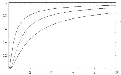
Figure 1: the top curve represents $\hat{C}_{3}(\omega)$, the middle one represents $\hat{C}_{1}(\omega)$, the bottom one represents $\hat{C}_{2}(\omega)$.

The coefficients $c_{1}=1$, $c_{2}=-4$ and $c_{+}=-\frac{1}{4}$. No such a precaution is necessary for the solution $\xi_{+}(\sigma)$ and the Runge-Kutta can start right at the point $\sigma=K$.The numerical results of $C_{1}(\omega)$, $C_{2}(\omega)$ and $C_{3}(\omega)$ are displayed in Fig.1, where we have introduced

$$\hat{C}_{1}(\omega)\equiv\frac{2}{3}C_{1}(\omega)e^{-2K\omega}=1-\frac{c}{\omega}+...,$$ (130)

$$\hat{C}_{2}(\omega)\equiv\frac{2}{3}C_{2}(\omega)e^{-2K\omega}=1-\frac{2c}{\omega}+...,$$ (131)

and

$$\hat{C}_{3}(\omega)\equiv 2C_{3}(\omega)e^{-2K\omega}=1-\frac{c}{2\omega}+...$$ (132)

with the last step of each equation following from the asymptotic expansions (83), (84) and (85). The comparison of the numerical results with the asymptotic expansions (130), (131) and (132) is shown in the table 1 and that with the small $\omega$ behaviors (91), (92) and (93) is shown in the table 2. The agreement is excellent. To gain more confidence on the numerical solutions of the differential equations (67), (68) and (69) for intermediate $\omega$, we checked the numerical code against a soluble model in which we base the covariant derivatives in (19) on the following AdS₂ metric

$$ds^{2}=\frac{1}{\cos^{2}\sigma}(d\tau^{2}+d\sigma^{2})$$ (133)

with $-\frac{\pi}{2}\leq\sigma\leq\frac{\pi}{2}$. The differential equations corresponding to (67), (68) and (69) can be reduced to hypergeometric equations and the exact forms of the $C$-coefficients of soluble model are derived in the appendix C. They read

$$C_{1}^{\rm sol.}(\omega)=C_{2}^{\rm sol.}(\omega)=\frac{3\omega^{2}}{\omega^{2}+1}\sinh\pi\omega$$ (134)

and

$$C_{3}^{\rm sol.}(\omega)=\frac{4\omega^{2}}{4\omega^{2}+1}\cosh\pi\omega.$$ (135)

We have

$$\ln\rho^{\rm sol.}(\omega)\equiv\ln\frac{3^{\frac{3}{2}}C_{3}^{\rm sol.}(\omega)^{4}}{C_{1}^{\rm sol.}(\omega)C_{2}^{\rm sol.}(\omega)^{\frac{1}{2}}\sinh^{\frac{5}{2}}\pi\omega}=\frac{1}{2\omega^{2}}+O(\frac{1}{\omega^{4}})$$ (136)

and

$$\int_{0}^{\infty}d\omega\ln\rho^{\rm sol.}(\omega)=0.$$ (137)

In Fig.2, we plot the function $\rho(\omega)$ of (106) along with that of the soluble model $\rho^{\rm sol.}(\omega)$. The small $\omega$ behavior of the former can be fitted to a polynomial

$$\rho(\omega)=2.19171\omega-3.4445\omega^{3}+6.21735\omega^{5}-10.8863\omega^{7}+17.5978\omega^{9},$$ (138)

consistent with (108). For large $\omega$, the products $\omega^{2}\rho(\omega)$ and $\omega^{2}\rho^{\rm sol.}(\omega)$ are tabulated in table 3 with both determined numerically. Both Fig.2 and Table 3 suggest that $\rho(\omega)$ falls off faster than $\rho^{\rm sol.}(\omega)$ for large $\omega$. An analytical demonstration requires extending the WKB approximation in appendix A to higher orders and will be rather tedious. Here we merely post our observation without offering a rigorous proof. The self-adaptive Simpson integration of $\ln\rho(\omega)$ yields

$$\int_{0}^{\infty}d\omega\ln\rho(\omega)\simeq-0.56534,$$ (139)

which, upon substitution into (117) leads to

$$\kappa_{1}=-1.33460.$$ (140)

The relative error in the numerical valuation of the elliptic functions is about $10^{-15}$ and that of the coefficients $C^{\rm sol.}(\omega)$’s extracted from our Runge-Kutta iteration is found below $10^{-11}$. Notice that the near singularity expansion of the trigonometric functions pertaining to the soluble model goes by the second power of $\epsilon$, while the same type of expansion of the elliptic functions pertaining to the parallel lines, (109) and (110), goes by the fourth power of $\epsilon$. Therefore the approximations (126)-(129) should work better for the parallel lines. Likewise is the numerical integration (139), the integrand of which vanishes faster than that of the soluble model at large $\omega$. For the soluble model, we found $2.39\times 10^{-8}$ in contrast to the exact value zero of (137). Consequently, the accuracy of our numerical algorithm should be amply sufficient for the six significant figures of the $\kappa$ value reported in this paper.

$\omega$	10	100	200	300	400	500	600	700
$\omega(1-\hat{C}_{1}(\omega))$	0.848635	0.847228	0.847217	0.847215	0.847214	0.847214	0.847214	0.847213
$\frac{\omega}{2}(1-\hat{C}_{2}(\omega))$	0.844365	0.847182	0.847205	0.847210	0.847211	0.847212	0.847212	0.847212
$2\omega(1-\hat{C}_{3}(\omega))$	0.846503	0.847205	0.847211	0.847212	0.847213	0.847213	0.847213	0.847213

Table 1: The large $\omega$ behaviors of the numerically generated $\hat{C}_{1}(\omega)$, $\hat{C}_{2}(\omega)$ and $\hat{C}_{3}(\omega)$

$\omega$	0.00001	0.00005	0.0001	0.0005	0.001	0.005	0.01
$\frac{C_{1}(\omega)}{\omega^{3}}$	10.16655701	10.16655704	10.16655711	10.16655950	10.16656698	10.16680621	10.16755383
$\frac{C_{2}(\omega)}{\omega^{3}}$	5.08327851	5.08327852	5.08327857	5.08328004	5.08328465	5.08343202	5.08389259
$\frac{C_{3}(\omega)}{\omega^{2}}$	4.00000000	4.00000001	4.00000006	4.00000143	4.00000574	4.00014355	4.00057424

Table 2: The small $\omega$ behaviors of the numerically generated $C_{1}(\omega)$, $C_{1}(\omega)$ and $C_{1}(\omega)$

$\omega$	10	100	200	300	400	500	600	700
$\omega^{2}\ln{\rho(\omega)}$	-0.000052	-0.000001	-0.000002	-0.000003	-0.000004	-0.000004	-0.000005	-0.000005
$\omega^{2}\ln{\rho^{sol.}(\omega)}$	0.493798	0.499938	0.499984	0.499993	0.499996	0.499997	0.499998	0.499999

Table 3: The large $\omega$ behaviors of $\rho(\omega)$ and $\rho^{\rm sol.}(\omega)$.

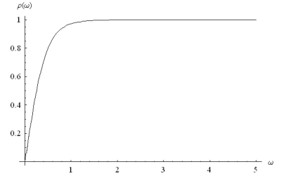
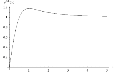
Figure 2: the left curve represents $\rho(\omega)$, while the right one represents $\rho^{\rm{sol.}}(\omega)$.

5 Determination of $\kappa_{2}$

To determine $\kappa_{2}$, we quote two formula of Ref.[16], one for a bosonic determinant and the other for a fermionic determinant. Consider a general 2d metric

$$ds^{2}=g_{\alpha\beta}d\sigma^{\alpha}d\sigma^{\beta}$$ (141)

with the scalar curvature $R$. Define the functional operator $\Delta_{M}\equiv M^{-1}(-\nabla^{2}+X)$ with $\nabla^{2}$ the Laplacian with respect to the metric (141) and ($M$, $X$) functions of coordinates. Varying $M$ amounts to a conformal transformation of the metric (141) and associated anomaly contributes a nontrivial finite term to the variation of the functional determinant of $\Delta_{M}$. We have

$$\left(\ln\frac{\det\Delta_{M})}{\det\Delta_{1}}\right)_{\rm fin.}=-\frac{1}{4\pi}\int d^{2}\sigma\sqrt{g}\Big{[}\ln M\left(\frac{1}{6}R-X\right)+\frac{1}{12}g^{\alpha\beta}\frac{\partial\ln M}{\partial\sigma^{\alpha}}\frac{\partial\ln M}{\partial\sigma^{\beta}}\Big{]}+\hbox{boundary terms},$$ (142)

Since we are always taking the difference between the parallel Wilson lines and the two single Wilson lines, the boundary terms cancel and we may integrate by part freely. For a Dirac operator with respect to the metric (141), $\gamma^{\alpha}\nabla_{\alpha}$, we define

$$\Delta_{\cal K}^{F}\equiv-({\cal K}^{-1}\gamma^{\alpha}\nabla_{\alpha})^{2}+{\cal K}^{-2}Y$$ (143)

with ${\cal K}$ and $Y$ functions of coordinates. The measure transformation formula corresponding to (142) reads.

$$\left(\ln\frac{\det\Delta_{\cal K}^{F})}{\det\Delta_{1}^{F}}\right)_{\rm fin.}=\frac{1}{2\pi}\int d^{2}\sigma\sqrt{g}\Big{[}\ln{\cal K}\left(\frac{1}{6}R+2Y\right)+\frac{1}{6}g^{\alpha\beta}\frac{\partial\ln{\cal K}}{\partial\sigma^{\alpha}}\frac{\partial\ln{\cal K}}{\partial\sigma^{\beta}}\Big{]}+\hbox{boundary terms},$$ (144)

where we have multiplied the integral in [16] by two, taking into account that $\Delta_{\cal K}^{F}$ here is a $2\times 2$ matrix in the spinor space.

Coming to the determinants we are interested in, metric (29)and metric (26) are all conformal with

$$g_{\alpha\beta}=e^{-2\chi}\delta_{\alpha\beta}$$ (145)

and the scalar curvature

$$R=2e^{2\chi}\delta^{\alpha\beta}\frac{\partial^{2}\chi}{\partial\sigma^{\alpha}\partial\sigma^{\beta}}.$$ (146)

We have $(\sigma_{0},\sigma_{1})=(\tau,\zeta)$ and $\chi=\ln\zeta$ for the single line, and $(\sigma_{0},\sigma_{1})=(\tau,\sigma)$ and $\chi=\ln(\sqrt{2}{\rm cn}\sigma)$ for the parallel lines. With the measure scaling functions $M=e^{2\chi}$ and ${\cal K}=e^{\chi}$, those functional operators of (31)-(37) without hats corresponds to $\Delta_{1}$ and $\Delta_{1}^{F}$ of eqs.(142) and (144) and that with hats to $\Delta_{M}$ and $\Delta_{\cal K}^{F}$ there. The ”mass square” $X$ of (142) equals to zero for $\Delta_{0}[{\cal C}_{1}]$ and $\Delta_{0}[{\cal C}_{2}]$, equals to 2 for $\Delta_{1}[{\cal C}_{1}]$ and $\Delta_{1}[{\cal C}_{2}]$ and equals to $4+R$ for $\Delta_{2}[{\cal C}_{2}]$. The ”mass” $Y$ of (144) equals to one for all fermionic determinants. It follows from (142) that

$$\left(\ln\frac{\det\Delta_{0}[{\cal C}_{1}]}{\det\hat{\Delta}_{0}[{\cal C}_{1}]}\right)_{\rm fin.}=-\frac{1}{12\pi}\int_{{\cal C}_{1}}d^{2}\sigma\delta^{\alpha\beta}\frac{\partial\chi}{\partial\sigma^{\alpha}}\frac{\partial\chi}{\partial\sigma^{\beta}}+\hbox{boundary terms},$$ (147)

$$\left(\ln\frac{\det\Delta_{0}[{\cal C}_{2}]}{\det\hat{\Delta}_{0}[{\cal C}_{2}]}\right)_{\rm fin.}=-\frac{1}{12\pi}\int_{{\cal C}_{2}}d^{2}\sigma\delta^{\alpha\beta}\frac{\partial\chi}{\partial\sigma^{\alpha}}\frac{\partial\chi}{\partial\sigma^{\beta}}+\hbox{boundary terms},$$ (148)

$$\left(\ln\frac{\det\Delta_{1}[{\cal C}_{1}]}{\det\hat{\Delta}_{1}[{\cal C}_{1}]}\right)_{\rm fin.}=-\frac{1}{12\pi}\int_{{\cal C}_{1}}d^{2}\sigma\delta^{\alpha\beta}\frac{\partial\chi}{\partial\sigma^{\alpha}}\frac{\partial\chi}{\partial\sigma^{\beta}}-\frac{1}{\pi}\int_{{\cal C}_{1}}d^{2}\sigma e^{-2\chi}\chi+\hbox{boundary terms},$$ (149)

$$\left(\ln\frac{\det\Delta_{1}[{\cal C}_{2}]}{\det\hat{\Delta}_{1}[{\cal C}_{2}]}\right)_{\rm fin.}=-\frac{1}{12\pi}\int_{{\cal C}_{2}}d^{2}\sigma\delta^{\alpha\beta}\frac{\partial\chi}{\partial\sigma^{\alpha}}\frac{\partial\chi}{\partial\sigma^{\beta}}-\frac{1}{\pi}\int_{{\cal C}_{2}}d^{2}\sigma e^{-2\chi}\chi+\hbox{boundary terms},$$ (150)

and

$$\left(\ln\frac{\det\Delta_{2}[{\cal C}_{2}]}{\det\hat{\Delta}_{2}[{\cal C}_{2}]}\right)_{\rm fin.}=\frac{11}{12\pi}\int_{{\cal C}_{2}}d^{2}\sigma\delta^{\alpha\beta}\frac{\partial\chi}{\partial\sigma^{\alpha}}\frac{\partial\chi}{\partial\sigma^{\beta}}-\frac{2}{\pi}\int_{{\cal C}_{2}}d^{2}\sigma e^{-2\chi}\chi+\hbox{boundary terms}.$$ (151)

where the subscript of the integration sign indicates the world sheet integration extends to. Similarly, the formula (144) implies that

$$\left(\ln\frac{|\det D_{F}[{\cal C}_{1}]|}{|\det\hat{D}_{F}[{\cal C}_{1}]|}\right)_{\rm fin.}=\frac{1}{24\pi}\int_{{\cal C}_{1}}d^{2}\sigma\delta^{\alpha\beta}\frac{\partial\chi}{\partial\sigma^{\alpha}}\frac{\partial\chi}{\partial\sigma^{\beta}}-\frac{1}{2\pi}\int_{{\cal C}_{1}}d^{2}\sigma e^{-2\chi}\chi+\hbox{boundary terms}$$ (152)

and

$$\left(\ln\frac{|\det D_{F}[{\cal C}_{2}]|}{|\det\hat{D}_{F}[{\cal C}_{2}]|}\right)_{\rm fin.}=\frac{1}{24\pi}\int_{{\cal C}_{2}}d^{2}\sigma\delta^{\alpha\beta}\frac{\partial\chi}{\partial\sigma^{\alpha}}\frac{\partial\chi}{\partial\sigma^{\beta}}-\frac{1}{2\pi}\int_{{\cal C}_{2}}d^{2}\sigma e^{-2\chi}\chi+\hbox{boundary terms}.$$ (153)

Substituting into (39) and (41) for the single line and the parallel lines, we find their contributions add up to zero in each case i.e. $W_{2}[{\cal C}_{1}]=W_{2}[{\cal C}_{2}]=0$. Consequently,

$$\kappa_{2}=0.$$ (154)

This, together with (140) leads to our final result (4).

6 Concluding remarks

As AdS/CFT has become an important reference to understand the observation of the strongly interacting quark-gluon plasma created by heavy ion collisions, it is critical to asses the robustness of the leading order prediction by exploring the next order correction in the expansion according to the inverse powers of the large ’t Hooft coupling $\lambda=N_{c}g_{\rm YM}^{2}$. The subleading terms of the expansion have been addressed in the literature in the context of the equation of state [25] and the shear viscosity [26][27]. This type of corrections comes from the $\alpha^{\prime 3}$ correction of the target space metric [28]. Its contribution is of the order $O(\lambda^{-3/2})$ relative to the leading order in the ${\cal N}=4$ SYM and is present only at nonzero temperature. In case of the expectation value of a Wilson loop operator, however, the dominant correction stems from the fluctuation of the world sheet around its minimum area and is suppressed only by $O(\lambda^{-1/2})$ relative to the leading order. It shows up at all temperatures and is more difficult to compute. The only attempts made in the literature in this regard include the strong coupling expansion of a single line, a circular loop and a spinning line at zero temperature [15][16][17][31]. These Wilson loops, though theoretically important, do not carry direct phenomenological implications.

In this work, we have extended the method in [17] to the fluctuations of the world sheet dual to a pair of parallel Wilson lines and have derived the next term of the strong coupling expansion of the heavy quark-antiquark potential in ${\cal N}=4$ SYM at zero temperature. We start with the determinant ratio for a single Wilson line and that for parallel lines in the static gauge, in which the fluctuations come from eight transverse bosonic coordinates and eight 2d Majorana fermions. Then we scaled the operators underlying the determinants, leaving a trivial measure for the associated spectral problem. The subleading term of the heavy quark potential is extracted from the combination (21), which consists of the spectral and the measure parts. A robust numerical result of the former is obtained and the contributions from measure change of each determinant cancel. We have,

$$V(r)=-\frac{a(\lambda)}{r}$$ (155)

with

$$a(\lambda)=\left\{\begin{array}[]{ll}\begin{gathered}\frac{4\pi^{2}}{\Gamma^{4}\left(\frac{1}{4}\right)}\frac{\sqrt{\lambda}}{r}\Big{[}1-\frac{1.33460}{\sqrt{\lambda}}+O\left(\frac{1}{\lambda}\right)\Big{]},\hskip 5.69046pt\hbox{for $\lambda>>1$}\\ \end{gathered}\hfill\\ \begin{gathered}\frac{\lambda}{4\pi r}\Big{[}1-\frac{\lambda}{2\pi^{2}}\left(\ln\frac{2\pi}{\lambda}-\gamma_{E}+1\right)+O(\lambda^{2})\Big{]},\hskip 5.69046pt\hbox{for $\lambda<<1$}\\ \end{gathered}\end{array}\right.$$ (156)

where the weak coupling expansion obtained in [13][29] from field theory is also included for completeness. The authors of [13] also worked out the strong coupling expansion under the ladder approximation in field theory,

$$V_{\rm ladder}(r)=-\frac{\sqrt{\lambda}}{\pi r}\left(1-\frac{\pi}{\sqrt{\lambda}}\right).$$ (157)

It is interesting to notice that our subleading term is of the same sign as theirs but the magnitude relative to the leading order is smaller in our result. In view of the range of the ’t Hooft coupling which was used for the RHIC phenomenology,

$$5.5<\lambda<6\pi$$ (158)

the correction to the leading order of the strong coupling may be significant in magnitude. One may define an effective coupling

$$\sqrt{\lambda^{\prime}}=\sqrt{\lambda}-1.33460$$ (159)

If $\lambda$ of (158) is replaced by $\lambda^{\prime}$, the range of the ’t Hooft coupling is shifted to

$$13.54<\lambda<32.22$$ (160)

At a nonzero temperature $T$, however, the order $O(\lambda^{-1/2})$ is not merely a redefinition of the coupling and the strong coupling expansion of the heavy quark potential becomes

$$V(r)\simeq-\frac{4\pi^{2}}{\Gamma^{4}\left(\frac{1}{4}\right)}\frac{\sqrt{\lambda}}{r}\Big{[}g_{0}(rT)-\frac{1.33460g_{1}(rT)}{\sqrt{\lambda}}+O\left(\frac{1}{\lambda}\right)\Big{]}$$ (161)

with $g_{0}(x)$ and $g_{1}(x)$ two functions satisfying the conditions $g_{0}(0)=g_{1}(0)=1$. The function $g_{0}(x)$ have been determined by the minimum area of the world sheet in the Schwarzschild-AdS${}_{5}\times$S⁵ target space [11]

$$ds^{2}=\frac{1}{z^{2}}\left(f(z)dt^{2}+d\vec{x}^{2}+\frac{1}{f(z)}dz^{2}\right)+d\Omega_{5}^{2}$$ (162)

with $f(z)=1-\pi^{4}T^{4}z^{4}$ and $t$ the Euclidean time. The one loop effective action underlying the function $g_{1}(x)$ has been developed in [30] and the methodology employed in this work can be readily generalized there.

While simple in practice, the static gauge we worked with suffers a problem. Though the combination (21) gives rise to a finite result, neither the UV divergence nor the conformal anomaly of each term on RHS of (21) vanishes. A less problematic gauge is the conformal gauge, in which the world sheet metric is not set to the induced metric at the beginning. One has to include the determinant of the longitudinal fluctuations and that of the ghost and an appropriate measure of the path integral. The contributions from the transverse bosons and fermions obtained in this paper will remain there, but other contributions including the measure change may be subtle to collect. It is important to carry out the parallel analysis in the conformal gauge to ascertain that our result in this paper is complete. Another alternative is the canonical quantization method employed in [31]. We hope to report our progress in this direction in near future.

Appendix A

To extract the large $\omega$ behavior of the coefficients $C_{1}(\omega)$, $C_{2}(\omega)$ and $C_{3}(\omega)$, we introduce $x\equiv\omega(K+\sigma)$ and $y\equiv\omega(K-\sigma)$. For $\sigma+K<<1$($K-\sigma<<1$), the solutions of the differential equations can be approximated by that of the equations for the single line, which extends to $x>>1$($y>>1$) for large $\omega$. The WKB approximation applies for $x>>1$ and $y>>1$. In case of eq.(69) with upper(lower) sign, the WKB solution can be extended all the way to the point $\sigma=K$($\sigma=-K$) and the requirement $y>>1$($x>>1$) may be relaxed. We match the single line solution and the WKB ones in the regions where both approximations apply.

Consider the equation (67) first. We start with the approximate solution near $\sigma=-K$

$$\eta_{1}\simeq 3u_{1}(x)$$ (163)

with $\sigma+K<<1$, where the coefficient 3 follows from the requirement (70). The asymptotic form for $x>>1$ reads

$$\eta_{1}\simeq\frac{3}{2}e^{x}\left(1-\frac{1}{x}\right)\simeq\frac{3}{2}e^{x-\frac{1}{x}}.$$ (164)

The WKB solution to be matched is given by

$$\eta_{1}\simeq\exp\left({\int^{\sigma}d\sigma^{\prime}\sqrt{\omega^{2}+\frac{1}{{\rm cn}^{2}\sigma^{\prime}}}}\right).$$ (165)

Expanding the square root for large $\omega$ and using the derivative formula

$$\frac{d}{d\sigma}\frac{{\rm sn}\sigma{\rm dn}\sigma}{{\rm cn}\sigma}=\frac{1}{2}\left(\frac{1}{{\rm cn}^{2}\sigma}+{\rm cn}^{2}\sigma\right)$$ (166)

we find that

$$\eta_{1}\simeq A\exp\left(\omega\sigma+\frac{1}{2\omega}\int_{-K}^{\sigma}\frac{d\sigma^{\prime}}{{\rm cn}^{2}\sigma^{\prime}}\right)\simeq A\left(\omega\sigma+\frac{{\rm sn}\sigma{\rm dn}\sigma}{\omega{\rm cn}\sigma}-\frac{1}{2\omega}\int_{-K}^{\sigma}d\sigma^{\prime}{\rm cn}^{2}\sigma^{\prime}\right)$$ (167)

with $A$ a constant to be determined. In the left matching region where $x>>1$ and $\sigma+K<<1$, the approximations

$$\frac{{\rm sn}(\sigma){\rm dn}(\sigma)}{{\rm cn}(\sigma)}\simeq-\frac{1}{K+\sigma}$$ (168)

and $\int_{-K}^{-\sigma}d\sigma^{\prime}{\rm cn}^{2}\sigma^{\prime}\simeq 0$ yield the coefficient $A=\frac{3}{2}e^{K\omega}$. In the right matching region where $K-\sigma<<1$ and $y>>1$, the WKB solution (167) becomes

$$\eta_{1}\simeq\frac{3}{2}e^{2K\omega-\frac{c}{\omega}}e^{-y+\frac{1}{y}},$$ (169)

where we have used the approximation

$$\frac{{\rm sn}(\sigma){\rm dn}(\sigma)}{{\rm cn}(\sigma)}\simeq\frac{1}{K-\sigma}$$ (170)

there and the constant

$$c=\frac{1}{2}\int_{-K}^{K}d\sigma{\rm cn}^{2}\sigma=\sqrt{2}\int_{0}^{1}dx\frac{x^{2}}{\sqrt{1-x^{4}}}=\frac{2\pi^{\frac{3}{2}}}{\Gamma^{2}\left(\frac{1}{4}\right)}.$$ (171)

Comparing with the expression of (62), we obtain that

$$\eta_{1}\simeq\frac{3}{2}e^{2K\omega-\frac{c}{\omega}}v_{1}(y).$$ (172)

The asymptotic behavior of (83) is extracted in the limit $y\to 0$ and the relation (113) for $\eta_{1}$ and $\xi_{1}$ follows.

The equation (68) can be treated similarly. We start with the same expression of (163) for $\eta_{2}(\sigma)$ near $\sigma=-K$ but replace the WKB solution (165) by

$$\eta_{2}\simeq\exp\left(\int^{\sigma}d\sigma^{\prime}\sqrt{\omega^{2}+\frac{1}{{\rm cn}^{2}\sigma^{\prime}}-{\rm cn}^{2}\sigma^{\prime}}\right)$$ (173)

Eqs.(167) and (169) become

$$\eta_{2}\simeq A\exp\left(\omega\sigma+\frac{1}{2\omega}\int_{-K}^{\sigma}\frac{d\sigma^{\prime}}{{\rm cn}^{2}\sigma^{\prime}}-\frac{1}{2\omega}\int_{-K}^{\sigma}d\sigma^{\prime}{\rm cn}^{2}\sigma^{\prime}\right)\simeq A\exp\left(\omega\sigma+\frac{{\rm sn}\sigma{\rm dn}\sigma}{{\rm cn}\sigma}-\frac{1}{\omega}\int_{-K}^{\sigma}d\sigma^{\prime}{\rm cn}^{2}\sigma^{\prime}\right)$$ (174)

with the same $A$ and

$$\eta_{2}(\sigma)\simeq\frac{3}{2}e^{2K\omega-\frac{2c}{\omega}}e^{-y+\frac{1}{y}}$$ (175)

for $y>>1$ and $K-\sigma<<1$. The asymptotic behavior (84) and the relation (113) for $(\eta_{2},\xi_{2})$ are extracted then.

Coming to eq.(69), the single line solution (163) remains approximating and we have

$$\eta_{+}\simeq 3u_{1}(x)$$ (176)

for $\sigma+K<<1$. The WKB solution it matches with for $x>>1$ reads

$$\eta_{+} \simeq \exp\left({\int^{\sigma}d\sigma^{\prime}\sqrt{\omega^{2}+\frac{1}{2{\rm cn}^{2}\sigma^{\prime}}-\frac{{\rm sn}\sigma^{\prime}{\rm dn}\sigma^{\prime}}{\sqrt{2}{\rm cn}^{2}\sigma^{\prime}}}}\right)$$ (177)

$$\simeq \frac{3}{2}\exp\left(K\omega+{\omega\sigma+\frac{1}{4\omega}\int^{\sigma}d\sigma^{\prime}\frac{1-\sqrt{2}{\rm sn}\sigma^{\prime}{\rm dn}\sigma^{\prime}}{{\rm cn}^{2}\sigma^{\prime}}}\right)$$

$$\simeq \frac{3}{2}\exp\left(K\omega+{\omega\sigma+\frac{1}{2\sqrt{2}\omega}\frac{\sqrt{2}{\rm sn}\sigma{\rm dn}\sigma-1}{{\rm cn}\sigma}-\frac{1}{4\omega}\int_{-K}^{\sigma}d\sigma^{\prime}{\rm cn}^{2}\sigma^{\prime}}\right)$$

and works all the way to the point $\sigma=K$. Near that point, we find

$$\eta_{+}\simeq\frac{3}{2}e^{2K\omega-\frac{c}{2\omega}-y}$$ (178)

Eqs.(85) and (114) follow from the form of $v_{0}(y)$, (80) and (81). The relation (115) is obtained starting with the WKB solution

$$\xi_{+}\simeq\sinh\left(\int_{\sigma}^{K}d\sigma^{\prime}\sqrt{\omega^{2}+\frac{1}{2{\rm cn}^{2}\sigma^{\prime}}-\frac{{\rm sn}\sigma^{\prime}{\rm dn}\sigma^{\prime}}{\sqrt{2}{\rm cn}^{2}\sigma^{\prime}}}\right)$$ (179)

and matching it to the approximate solution $v_{1}(x)$ for $K+\sigma<<1$ and $x>>1$.

Appendix B

The differential equation (67) at $\omega=0$ can be converted to a hypergeometric equation by the transformation

$$x={\rm cn}^{4}\sigma\qquad\phi(\sigma)=\sqrt{x}f(x),$$ (180)

i.e.

$$x(1-x)\frac{d^{2}f}{dx^{2}}+\left(\frac{7}{4}-\frac{9}{4}x\right)\frac{df}{dx}-\frac{3}{8}f=0.$$ (181)

We have

$$\bar{\eta}_{1}(\sigma)=2{\rm cn}^{2}\sigma F\left(\frac{1}{2},\frac{3}{4};\frac{7}{4};{\rm cn}^{4}\sigma\right)$$ (182)

and $\bar{\xi}_{1}(\sigma)=\bar{\eta}_{1}(-\sigma)$. It follows from the formula

$$\frac{d}{dz}F(a,b;c;z)=\frac{ab}{c}F(a+1,b+1;c+1;z),$$ (183)

$$F(a,b;c;1)=\frac{\Gamma(c)\Gamma(c-a-b)}{\Gamma(c-a)\Gamma(c-b)}$$ (184)

for ${\rm Re}(c-a-b)>0$ and

$$F(a,b;c;1-\epsilon)=\frac{\Gamma(c)\Gamma(a+b-c)}{\Gamma(a)\Gamma(b)}\epsilon^{c-a-b}+...$$ (185)

for ${\rm Re}(c-a-b)<0$ and $\epsilon>0$ that the Wronskian

$$W[\bar{\eta}_{1},\bar{\xi}_{1}] = -2\lim_{\epsilon\to 0^{+}}\bar{\eta}_{1}(-\epsilon)\bar{\eta}_{1}^{\prime}(-\epsilon)=-\frac{48}{7\sqrt{2}}\frac{\Gamma\left(\frac{7}{4}\right)\Gamma\left(\frac{1}{2}\right)}{\Gamma\left(\frac{5}{4}\right)\Gamma(1)}\frac{\Gamma\left(\frac{11}{4}\right)\Gamma\left(\frac{1}{2}\right)}{\Gamma\left(\frac{3}{2}\right)\Gamma\left(\frac{7}{4}\right)}$$ (186)

$$= -\frac{72\pi^{\frac{3}{2}}}{\Gamma^{2}\left(\frac{1}{4}\right)}$$

Divided by -3, we derive (91).

With the same transformation (180), eq.(68) becomes

$$x(1-x)\frac{d^{2}f}{dx^{2}}+\left(\frac{7}{4}-\frac{9}{4}x\right)\frac{df}{dx}-\frac{1}{4}f=0.$$ (187)

We have

$$\bar{\eta}_{2}(\sigma)=2{\rm cn}^{2}\sigma F\left(1,\frac{1}{4};\frac{7}{4};{\rm cn}^{4}\sigma\right)$$ (188)

and $\bar{\xi}_{2}(\sigma)=\bar{\eta}_{2}(-\sigma)$. It follows from (183)-(185) that the Wronskian

$$W[\bar{\eta}_{2},\bar{\xi}_{2}] = -2\lim_{\epsilon\to 0^{+}}\bar{\eta}_{2}(-\epsilon)\bar{\eta}_{2}^{\prime}(-\epsilon)=-\frac{32}{7\sqrt{2}}\frac{\Gamma\left(\frac{7}{4}\right)\Gamma\left(\frac{1}{2}\right)}{\Gamma\left(\frac{3}{4}\right)\Gamma\left(\frac{3}{2}\right)}\frac{\Gamma\left(\frac{11}{4}\right)\Gamma\left(\frac{1}{2}\right)}{\Gamma(2)\Gamma\left(\frac{5}{4}\right)}$$ (189)

$$= -\frac{36\pi^{\frac{3}{2}}}{\Gamma^{2}\left(\frac{1}{4}\right)}$$

and (92) is obtained as $-W[\bar{\eta}_{2},\bar{\xi}_{2}]/3$. Using the series representation of the hypergeometric function, we find that

$$\bar{\eta}_{1}=\frac{3}{2}x^{-\frac{1}{4}}\int_{0}^{x}\frac{dx^{\prime}x^{\prime-\frac{1}{4}}}{\sqrt{1-x^{\prime}}}=\frac{3\sqrt{2}}{{\rm cn}\sigma}\int_{-K}^{\sigma}d\sigma^{\prime}{\rm cn}^{2}\sigma^{\prime}.$$ (190)

But we fail to find a similar expression for $\bar{\eta}_{2}(\sigma)$.

As to $\bar{C}_{3}(0)$, we notice that the solution of the 1st order differential equation

$$\sqrt{2}{\rm cn}\sigma\frac{d\psi}{d\sigma}+\psi=0$$ (191)

also solves eq.(69) with the upper sign. The eq.(191) can be solved readily and we obtain

$$\psi(\sigma)=B\sqrt{\frac{\sqrt{2}{\rm dn}\sigma-{\rm sn}\sigma}{\sqrt{2}{\rm dn}\sigma+{\rm sn}\sigma}}$$ (192)

with $B$ a constant, where we have used the indefinite integral

$$\int d\sigma\frac{1}{{\rm cn}\sigma}=-\frac{1}{\sqrt{2}}\ln\frac{\sqrt{2}{\rm dn}\sigma-{\rm sn}\sigma}{\sqrt{2}{\rm dn}\sigma+{\rm sn}\sigma}+{\rm const.}$$ (193)

as can be verified by taking derivatives of both sides. Setting the constant $B=2$, we find that the function $\psi(\sigma)$ satisfies the boundary condition of $\bar{\xi}_{+}(\sigma)$ at $\sigma=K$ and therefore $\bar{\xi}_{+}(\sigma)=\psi(\sigma)$. As $\sigma\to-K$,

$$\bar{\xi}_{+}(\sigma)=\frac{4}{\sigma+K}+...$$ (194)

and we end up with $\bar{C}_{3}(0)=4$.

Appendix C

In this appendix, we present the details of the soluble model which is introduced to check our numerical algorithm. The model is largely motivated by the work in [32]. We shall use the same symbols $(\eta,\xi)$ for the solutions of the counterparts of the differential equations (67), (68) and (69). Because the scalar curvature of the metric (133) is $R=-2$, the counterparts of (67) and (68) are the same. Consequently, $D_{1}(\omega)=D_{2}(\omega)$ and $(\eta_{1},\xi_{1})=(\eta_{2},\xi_{2})$ in this case. The counterpart of the eq.(67) or (68) reads,

$$-\frac{d^{2}\phi}{d\sigma^{2}}+\left(\omega^{2}+\frac{2}{\cos^{2}\sigma}\right)\phi=0$$ (195)

and has the same set of indexes at the regular points $\sigma=\pm\frac{\pi}{2}$ as that of (67). The symmetry property (74), the relation (80) and the formula (125) remains valid. The solution $\eta_{1}(\sigma)$, specified by the boundary conditions (70) with $K$ replaced by $\frac{\pi}{2}$ is

$$\eta_{1}(\sigma)=(\omega\cos\sigma)^{2}F\left(1+i\frac{\omega}{2},1-i\frac{\omega}{2};\frac{5}{2};\cos^{2}\sigma\right)$$ (196)

and $\xi(\sigma)=\eta(-\sigma)$. It follows from (125), the formula (183) -(185) for hypergeometric functions that

$$W[\eta_{1},\xi_{1}] = -2\lim_{\epsilon\to 0^{+}}\eta_{1}(-\epsilon)\eta_{1}^{\prime}(-\epsilon)=-\frac{\omega^{4}(\omega^{2}+4)}{5}\frac{\Gamma\left(\frac{5}{2}\right)\Gamma\left(\frac{7}{2}\right)\Gamma^{2}\left(\frac{1}{2}\right)}{\Gamma\left(\frac{3+i\omega}{2}\right)\Gamma\left(2+i\frac{\omega}{2}\right)\Gamma\left(\frac{3-i\omega}{2}\right)\Gamma\left(2-i\frac{\omega}{2}\right)}$$ (197)

$$= -\frac{9\omega^{3}}{\omega^{2}+1}\sinh\pi\omega$$ (198)

Divided by $-3\omega$ we end up with (134). The nonzero component of the spin connection corresponding to the metric (133) is $\omega_{\tau}^{01}=\tan\sigma$ and the counterpart of eq(69) with the upper sign reads

$$\frac{d^{2}\phi}{d\sigma^{2}}-\left(\omega^{2}+\frac{1}{1+\sin\sigma}\right)\phi=0.$$ (199)

The equation (199) can be reduced to a hypergeometric equation and the solutions satisfying the boundary conditions (70), (72) and (73) (with $K$ replaced by $\frac{\pi}{2}$) read

$$\eta_{+}=2\omega^{2}(1+\sin\sigma)F\left(1+i\omega,1-i\omega;\frac{5}{2};\frac{1+\sin\sigma}{2}\right)$$ (200)

and

$$\xi_{+}=\frac{1}{\sqrt{2}}(1+\sin\sigma)\sqrt{1-\sin\sigma}F\left(\frac{3}{2}+i\omega,\frac{3}{2}-i\omega;\frac{3}{2};\frac{1-\sin\sigma}{2}\right).$$ (201)

Their Wronskian

$$W[\eta_{+},\xi_{+}] = \eta_{+}\left(\frac{\pi}{2}\right)\xi^{\prime}_{+}\left(\frac{\pi}{2}\right)=-4\omega^{2}F\left(1+i\omega,1-i\omega;\frac{5}{2};1\right)$$ (202)

$$= -4\omega^{2}\frac{\Gamma\left(\frac{5}{2}\right)\Gamma\left(\frac{1}{2}\right)}{\Gamma\left(\frac{3}{2}+i\omega\right)\Gamma\left(\frac{3}{2}-i\omega\right)}=\frac{3\omega^{2}}{\omega^{2}+\frac{1}{4}}\cosh\pi\omega.$$

The eq.(135) follows then from (202) and (81).