Amplitudes in the Coulomb
interference region of pp and p$\bar{\rm p}$ scattering

Abstract

We discuss the determination of the parameters of the pp and p$\bar{\rm p}$ amplitudes for the description of scattering in the Coulomb interference region. We put enphasis on the possibility that the effective slope observed in the differential cross section is formed by different exponential slopes in the real and imaginary amplitudes (called $B_{R}$ and $B_{I}$). For this purpose we develop a more general treatment of the Coulomb phase. We analyse the differential cross section data in the range from 19 to 1800 GeV with four parameters ($\sigma~{},~{}\rho~{},~{}B_{I}~{},~{}B_{R}$ ), and observe that we cannot obtain from the data a unique determination of the parameters. We investigate correlations in pairs of the four quantities, showing ranges leading to the smaller $\chi^{2}$ values.

In the specific case of p$\bar{\rm p}$ scattering at 541 GeV, we investigate the measurements of event rate dN/dt at low $|t|$ augier in terms of the Coulomb interference with exponentially decreasing nuclear amplitudes. The analysis allows a determination of the normalization factor connecting the event rate with the absolute cross section.

I Introduction

The experiments in the high energy accelerators of Cern and Fermilab in the period from 1960 to 1990 collected data on the differential cross sections $d\sigma/dt$ for the systems pp and p$\bar{\rm p}$ at the center of mass energies $\sqrt{s}=20-1800$ GeV . Along almost 50 years since the beginning of these studies of high energy hadronic scattering, many theoretical models were developed, but the experimental data stopped increasing in quantity or quality, as the accelerators were discontinued. The phenomenology and theoretical treatments of these systems are thus restricted in several aspects. The theoretical literature is enormous, now with increased interest due to the higher energy data that will come from LHC operation fiore , and in the present work we do not analyse or compare the many dynamical and phenomenological efforts.

To study of the dynamics that governs the processes, it is necessary to disentangle the squared moduli of complex quantities that represent the measured quantities in terms of the imaginary and real parts, which are intrinsically combined with the Coulomb contribution.

In the region of small momentum transfers $|t|$, the intense Coulomb amplitude added to the nuclear interaction creates an interference that is observable in the $|t|$ distribution in $d\sigma/dt$. This Coulomb interference region of low $|t|$ values goes typically up to $|t|=0.01~{}{\rm GeV}^{2}$, but we show that the form of $d\sigma/dt$ in general can actually be described in terms of simple exponential real and imaginary nuclear amplitudes well beyond this range.

In previous analysis of the pp and p$\bar{\rm p}$ data, the real and imaginary nuclear amplitudes were considered as having the same exponential dependence $\exp{(Bt/2)}$ , where $B$ is the slope of the log plot of $d\sigma/dt$ . This simplifying assumption is not adequate, according to dispersion relations EF2007 and according to the theorem of A. Martin Martin that says that the position of the zero of the real amplitude is close and approaches $t=0$ as the energy increases. Both results indicate that the slope of the real amplitude should be larger than that of the imaginary one, and in the present work we investigate the description of the Coulomb interference region allowing for different real and imaginary slopes. We review the scattering data in cases where this kind of information can be looked for.

In Sec. II we review the expressions for the observable quantities in the forward region, and obtain the expression of the intervening relative phase for the more general case of different slopes for the real and imaginary amplitudes. In Sec. III we analyse the differential cross sections for the energies in pp and p$\bar{\rm p}$ scattering where data are more favorable. In Sec. IV we present some remarks and conclusions.

II Low $|t|$ region and Coulomb phase

II.1 Description of scattering for small $|t|$

In elastic pp and p$\bar{\rm p}$ collisions, the combined nuclear and coulomb amplitudes is written

$$F^{C+N}(s,t)=F^{C}(s,t)e^{i\alpha\Phi(s,t)}+F^{N}(s,t)~{},$$ (1)

where $F^{C}$ is the Coulomb part

$$F^{C}=(-/+)~{}\frac{2\alpha}{|t|}~{}F^{2}_{\rm proton}$$ (2)

with the proton electromagnetic form factor

$$F_{\rm proton}=(0.71/(0.71+|t|))^{2}~{},$$ (3)

associated to a relative phase $\Phi$, and $F^{N}$ is the strong interaction complexe amplitude

$$F^{N}(s,t)=F^{N}_{R}(s,t)+i~{}F^{N}_{I}(s,t)~{}.$$ (4)

The phase $\Phi$ was initially studied by West and Yennie WY , and different evaluations have been worked out by several authors selyugin ; petrov ; KL . In the present work we extend these investigations considering the possibility of different slopes for the real and imaginary amplitudes.

In the normalization that we use nicolescu the differential cross section is written

$$\frac{d\sigma}{dt}=\pi|F^{C+N}(s,t)|^{2}=\pi|F^{C}(s,t)e^{i\alpha\Phi(s,t)}+F^{N}_{R}(s,t)+iF^{N}_{I}(s,t)|^{2}~{}.$$ (5)

For small angles we can approximate

$$F^{N}(s,t)\approx F^{N}_{R}(s,0)e^{B_{R}t/2}+iF^{N}_{I}(s,0)e^{B_{I}t/2}~{}.$$ (6)

The slopes $B_{R}$ and $B_{I}$ are usually treated as having equal values. In the present work we allow $B_{R}\neq B_{I}$.

The parameter

$$\rho=\frac{F^{N}_{R}(s,0)}{F^{N}_{I}(s,0)}~{},$$ (7)

the optical theorem

$$\sigma=4\pi~{}(0.389)~{}{\rm Im}~{}{F^{N}_{I}(s,0)}~{},$$ (8)

and the slopes $B_{R}$, $B_{I}$ are used to parametrize the differential cross section for small $|t|$ . In these expressions, $\sigma$ is in milibarns and the amplitudes $F_{R}$, $F_{I}$ are in $\nobreak\,\mbox{GeV}^{-2}$ .

For low $|t|$ , eq. (6) leads to the approximate form

$$\frac{d\sigma}{dt}=\bigg{|}\frac{d\sigma}{dt}\bigg{|}_{t=0}~{}e^{Bt}~{},$$ (9)

with

$$B=\frac{\rho^{2}B_{R}+B_{I}}{1+\rho^{2}}~{}$$ (10)

as the usual slope observed in the data of $d{\sigma}/dt$.

II.2 The Coulomb phase

Here we derive an expression for the phase appropriate for cases with $B_{R}\neq B_{I}$.

The starting point is the expression for the phase obtained by West and Yennie WY

$$\Phi(s,t)=(-/+)\Bigg{[}\ln\bigg{(}-\frac{t}{s}\bigg{)}+\int_{-4p^{2}}^{0}\frac{dt^{\prime}}{|t^{\prime}-t|}\bigg{[}1-\frac{F^{N}(s,t^{\prime})}{F^{N}(s,t)}\bigg{]}~{},\Bigg{]}$$ (11)

where the signs $(-/+)$ are applied to the choices pp/p$\bar{\rm p}$ respectively. The quantity $p$ is the proton momentum im center of mass system, and at high energies $4p^{2}\approx s$ .

For small $|t|$, assuming that $F^{N}(s,t^{\prime})$ keeps the same form for large $|t^{\prime}|$ (this approximation should not have practical importance for the results), we have

$$\frac{F^{N}(s,t^{\prime})}{F^{N}(s,t)} = \frac{F_{R}^{N}(s,0)e^{B_{R}t^{\prime}/2}+i~{}F_{I}^{N}(s,0)e^{B_{I}t^{\prime}/2}}{F_{R}^{N}(s,0)e^{B_{R}t/2}+i~{}F_{I}^{N}(s,0)e^{B_{I}t/2}}$$ (12)

$$= \frac{c}{c+i}~{}e^{B_{R}(t^{\prime}-t)/2}+\frac{i}{c+i}~{}e^{B_{I}(t^{\prime}-t)/2}~{},$$

where

$$c\equiv\rho e^{(B_{R}-B_{I})t/2}~{}.$$ (13)

The calculation is explained in detail in the appendix. The integrals that appear in the evaluation of eq. (11) are reduced to the form KL

$$I(B)=\int_{-4p^{2}}^{0}\frac{dt^{\prime}}{|t^{\prime}-t|}\bigg{[}1-e^{B(t^{\prime}-t)/2}\bigg{]}~{}$$ (14)

that is solved in terms of exponential integrals abramowitz as

$$I(B)=E_{1}\big{[}\frac{B}{2}\bigg{(}4p^{2}+t\bigg{)}\big{]}-E_{i}\big{[}-\frac{Bt}{2}\big{]}+\ln\big{[}\frac{B}{2}\bigg{(}4p^{2}+t\bigg{)}\big{]}-\ln\big{[}-\frac{Bt}{2}\big{]}+2\gamma~{}.$$ (15)

The real part of the phase is then written

$$\Phi(s,t)=(-/+)\Bigg{[}\ln\bigg{(}-\frac{t}{s}\bigg{)}+\frac{1}{c^{2}+1}\bigg{[}c^{2}I(B_{R})+I(B_{I})\bigg{]}\Bigg{]}~{},$$ (16)

and this expression in introduced into eq. ( 5 ) .

III Analysis of experimental data

With $\sigma$ in mb and $t$ in GeV² the practical expession for $d\sigma/dt$ in terms of the parameters $\sigma$, $\rho$ , $B_{I}$ and $B_{R}$ is

$$\frac{d\sigma}{dt}=0.389~{}\pi\Bigg{[}\bigg{[}\frac{\rho~{}\sigma~{}e^{B_{R}t/2}}{0.389\times 4\pi}+F^{C}\cos(\Phi)\bigg{]}^{2}+\bigg{[}\frac{\sigma~{}e^{B_{I}t/2}}{0.389\times 4\pi}+F^{C}\sin(\Phi)\bigg{]}^{2}\Bigg{]}~{},$$ (17)

where by $\Phi$ we mean the real part given in eq. (16), written

$$\Phi=(-/+)~{}\alpha~{}\Bigg{[}\ln\bigg{(}-\frac{t}{s}\bigg{)}+Z_{R}\Bigg{]}~{},$$ (18)

where

$$Z_{R}=\frac{1}{1+c^{2}}\bigg{[}c^{2}I(B_{R})+I(B_{I})\bigg{]}~{},$$ (19)

with $c$ given in Eq. (13).

At high energies and small $|t|$ we simplify

$$4p^{2}+t\rightarrow s$$

and then the functional form of $I(B)$ is written

$$I(B)=E_{1}\bigg{(}\frac{Bs}{2}\bigg{)}-E_{i}\bigg{(}-\frac{Bt}{2}\bigg{)}+\ln\bigg{(}\frac{Bs}{2}\bigg{)}-\ln\bigg{(}-\frac{Bt}{2}\bigg{)}+2\gamma~{}.$$ (20)

We have used fitting programs (Cern Minuit-PAW and Numerical Recipes) to obtain correlations for the four parameters ( $\sigma,\rho,B_{R},B_{I}$ ), for some values of energy where the data from CERN and Fermilab databasis have more quality and quantity. Below we present these cases.

It is important to remark that the results obtained in the fittings in general depend strongly on the set of data of low $|t|$ selected for the analysis of the Coulomb interference region. This shows that the data accumulated in these experiments are not detailed and regular enough to allow precise determination of the amplitudes in the forward direction.

We stress that in this paper we do not intend to give new better values for parameters. Instead, we show that the analysis of the data leads to rather ample possibilities.

The values of forward scattering parameters for pp scattering at Fermilab and Cern ISR energies given in the standard literature are given in Table 1. The data at $\sqrt{s}=19.4$ GeV come from Fermilab , and that at 23.5 - 62.5 GeV are from the Cern ISR, with a review by Amaldi and Schubert amaldi .

Table 1: Forward scattering parameters found in the literature. At 1800 GeV the data values $1800^{(a)}$ and $1800^{(b)}$ correspond to the experiments E710 and E741 in Fermilab

$\sqrt{s}$ (GeV)	$\sigma$ (mb)	$\rho$	$B({\rm GeV}^{-2})$
19.4	$38.98\pm 0.04$	$0.019\pm 0.016$	$11.74\pm 0.04$
23.5	$38.94\pm 0.17$	$0.02\pm 0.05$	$11.80\pm 0.30$
30.7	$40.14\pm 0.17$	$0.042\pm 0.011$	$12.20\pm 0.30$
44.7	$41.79\pm 0.16$	$0.0620\pm 0.011$	$12.80\pm 0.20$
52.8	$42.67\pm 0.19$	$0.078\pm 0.010$	$12.87\pm 0.14$
62.5	$43.32\pm 0.23$	$0.095\pm 0.011$	$13.02\pm 0.27$
541	$62.20\pm 1.5$	$0.135\pm 0.015$	$15.52\pm 0.07$
$1800^{(a)}$	$72.20\pm 2.7$	$0.140\pm 0.069$	$16.72\pm 0.44$
$1800^{(b)}$	$80.03\pm 2.24$	$0.15$	$16.98\pm 0.25$

Our determination of the parameters is described below. In Table 2 we collect our results. It is remarkable that the obtained $\chi^{2}$ values are very small.

Table 2: Forward scattering parameters obtained in our analysis.

$\sqrt{s}$ (GeV)	$\sigma({\rm mb})$	$\rho$	$B_{I}({\rm GeV}^{-2})$	$B_{R}({\rm GeV}^{-2})$	$\beta=B_{R}/B_{I}$	$\chi^{2}$
$19.4$	$40.379\pm 0.069$	$0.019$ (fixed)	$14.539\pm 0.262$	$B_{I}~{},~{}2B_{I}$	1   ,  2	$1.299$
$23.5$	$39.821\pm 1.479$	$0.0186\pm 0.0137$	$14.912\pm 9.246$	$35.220\pm 177.57$	$2.36$	$0.2952$
$30.7$	$40.024\pm 0.047$	$0.027({\rm fixed})$	$11.784\pm 0.239$	$B_{I}~{},~{}2B_{I}$	$1~{},~{}2$	$0.5361$
$44.7$	$41.839\pm 0.291$	$0.0543\pm 0.0037$	$12.976\pm 0.631$	$16.132\pm 15.509$	$1.243$	$0.6110$
$52.8$	$42.576\pm 0.820$	$0.0799\pm 0.0086$	$13.414\pm 1.847$	$14.113\pm 33.684$	$1.052$	$0.1138$
$62.5$	$43.298\pm 0.159$	$0.0867\pm 0.0034$	$13.299\pm 0.358$	$13.900\pm 10.007$	$1.045$	$0.5389$

III.1 pp scattering at $\sqrt{s}$ = 19.4 GeV

Considering only Kuznetsov kuznetsov and Schiz schiz measurements, we have a total of 69+134 points at 19.4 GeV. We have fittted the set of the first 61 points from Kuznetsov plus the 12 first ones from Schiz, covering the range

$$0.00066\leq|t|\leq 0.0395~{}.$$

According to the information in the Durham Data Basis about this experiment, it is known that fittings that include the points of Kuznetsov lead no negative values of the parameter $\rho$. We then fix the value $\rho=0.019$ (taken from Table 1) and leave free the other parameters. The results are given in Table 2 . The data and the solution of fitting are shown if Fig. 1 . It is remarkable that the choices $B_{R}=B_{I}$ and $B_{R}=2~{}B_{I}$ lead to the same $\chi^{2}$.

Figure 1: Data from Kuznetsov (61 points) kuznetsov and Schiz (12 points)schiz are fitted to determine parameters at 19.4 GeV. We fix $\rho=0.019$ (taken from Table 1) because fittings including Kuznetsov’s measurements lead to negative value of $\rho$.

III.2 pp scattering at $\sqrt{s}$ = 23.542 GeV

At 23.542 GeV there are 31 experimental points amos . In order to obtain smaller values of $\chi^{2}$, the fitting was made using the first 17 points, with $|t|$ in the interval

$$0.00037\leq|t|\leq 0.00395~{},$$

leading to the results given in Table 2. The central value obtained for the ratio $\beta$ is

$$\beta=B_{R}/B_{I}=2.36~{}.$$

The same value $\chi^{2}=0.2952$ is obtained for any $\beta=B_{R}/B_{I}$ in the interval from 1.22 to 4.91 .

The plot of the 31 points together with the line obtained with fitting of 17 points are shown in Fig 2. Correlations between parameters $\rho$ and $\beta$ are shown in the RHS, with level curves of $\chi^{2}$. This plot is made fixing the values of $\rho$ and $\beta$, so that only 2 parameters are free (this explains the relation $0.2952=0.25587\times(17-2)/(17-4)$ in the values of $\chi^{2}$). The two different algorithms lead to distinct ranges in $\beta$, indicating that the data have poor definition for this quantity.

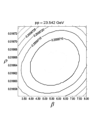
Figure 2: Data at 23.542 GeV . The first 17 points are fitted with expressions of Coulomb interference and exponential forms for the amplitudes. The graph in the RHS shows the regions of variation of $\rho$ and $\beta=B_{R}/B_{I}$ that correspond to small values of $\chi^{2}$ while the quantities $\sigma$ and $B_{I}$ are free.

III.3 pp scattering at $\sqrt{s}$ = 30.632 GeV

Although the data (32 points) of pp scattering at 30.632 GeV amos look regular , we have difficulties to find values for the parameters, although $\chi^{2}$ comes out small. The value 0.042 given for $\rho$ in Table 1 does not seem to be realistic, as our procedure leads to smaller values. With the value $\rho=0.027$ fixed, the ratio $\beta=B_{R}/B_{I}$ can vary in a large interval, keeping the same $\chi^{2}=0.5361$. The data, fitted with Coulomb interference expressions and exponential amplitudes, are shown in Fig. 3 and the parameters are given in Table 2.

Figure 3: Data at 30.632 GeV . The 32 points are fitted with expressions of Coulomb interference and exponential forms for the amplitudes.

III.4 pp scattering at $\sqrt{s}$ = 44.699 GeV

The 230 data points of the experiment at $\sqrt{s}=44.699$ GeV extending up to $|t|\approx 7~{}{\rm GeV}^{2}$ are presented in the report by Amaldi and Schubert amaldi . The forward part, with 40 points, up to $|t|\approx 0.02~{}{\rm GeV}^{2}$, is very well fitted by the Coulomb interference formula, as shown in Fig. 4, with $\chi^{2}=0.6110$. The parameters are given in Table 2 .

Any value of the ratio $\beta={B_{R}}/{B_{I}}$ in the range

$$0.601~{}\leq~{}\frac{B_{R}}{B_{I}}~{}\leq~{}1.667$$

leads to the same value 0.6110 for $\chi^{2}$.

Figure 4: Fitting of the 40 points with lowest $|t|$ at 44.699 GeV .

In Fig. 5 we show the solution for low $|t|$ together with higher $|t|$ data, exhibiting the peculiar behaviour of the amplitudes deviating from the simple exponential dependence. In the plot with all 230 points , the dotted line shows the fitting obtained with the parametrization used in a previous work pereira_ferreira . The parameters obtained in this case are $\sigma=42.10$ mb, $\rho=0.094$, $B_{I}=12.22~{}{\rm{GeV}}^{-2}$, and $B_{R}=24.43~{}{\rm{GeV}}^{-2}$. It is interesting that the description of the whole $|t|$ range leads to a definite indication for $B_{R}\approx 2~{}B_{I}$.

Figure 5: The extended dashed line representing the fitting at very low $|t|$ is plotted together with measurements at higher $|t|$, at $\sqrt{s}=44.699$ GeV. The dotted line shows a fitting of the whole set of points pereira_ferreira .

Correlations between parameters are shown in Fig 6, with level curves of $\chi^{2}$ . The two plots show respectively the correlations between $\rho$ and $\beta$ and between $\sigma$ and $\beta$. of

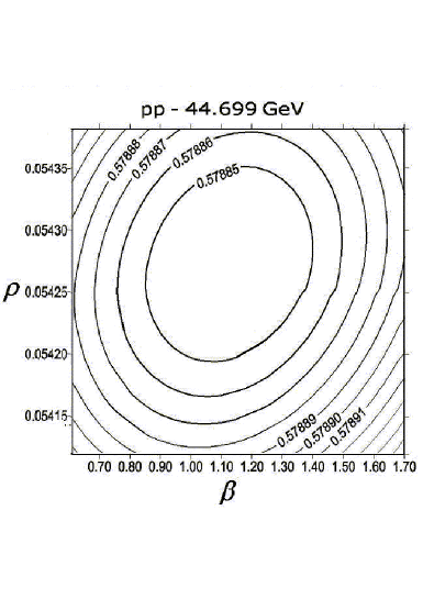
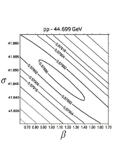
Figure 6: Ranges of values of parameters at $\sqrt{s}=44.699$ GeV that lead to small values of $\chi^{2}$. The searches are made fixing the two values in the axes of the plots, while the other two parameters are free.

With fixed $B_{R}/B_{I}=2$ we obtain $\chi^{2}=0.6111$ , with $\sigma=41.819\pm 0.089$ , $\rho=0.0543\pm 0.0029$ , $B_{I}=12.943\pm 0.406$ .

III.5 pp scattering at $\sqrt{s}$ = 52.806 GeV

Fig. 7 shows the forward data at $\sqrt{s}=52.806$ GeV (34 points) amos and our fitting with Coulomb interference expressions using the first 20 points.

Figure 7: Data of pp forward scattering at 52.8 GeV fitted with Coulomb interference formulae.

Correlations between parameters are shown in Fig. 8 , with level curves of $\chi^{2}$ . The two plots are built fixing the two parameters in the axes while the other two parameters are found by fitting.

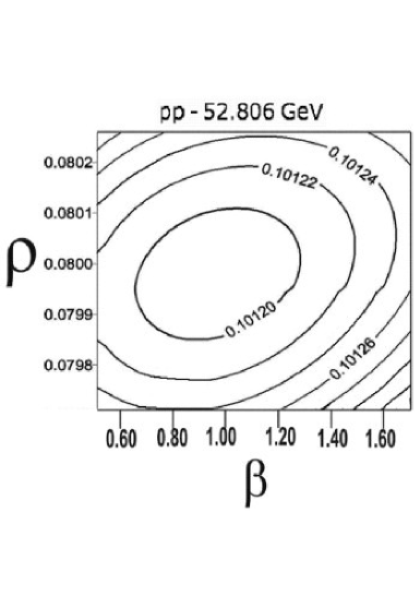
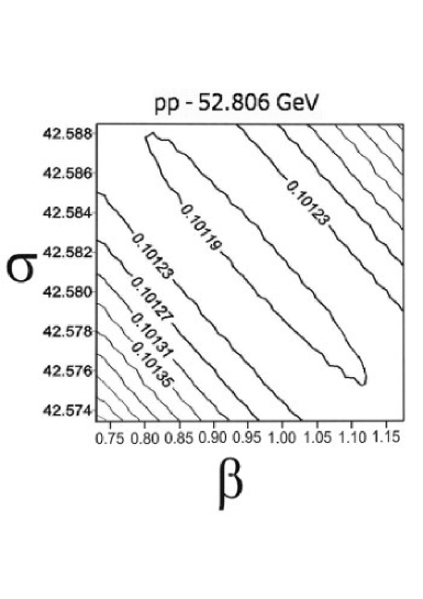
Figure 8: Correlations between pairs of parameters in pp scattering at 52.8 GeV.

The parameters obtained with 20 points in the interval

$$0.00107\leq|t|\leq 0.02235$$

are given in Table 2   . The ratio $\beta={B_{R}}/{B_{I}}$ with any value in the range

$$0.702\leq B_{R}/B_{I}\leq 1.214~{}$$

leads to the same value 0.1138 for $\chi^{2}$.

With fixed $B_{R}/B_{I}=2$ we obtain $\chi^{2}=0.1140$ , with $\sigma=42.543\pm 0.057$ , $\rho=0.0801\pm 0.0047$ , $B_{I}=13.347\pm 0.214$ .

III.6 pp at $\sqrt{s}$ = 62.5 GeV

Fig. 9 shows the data (138 points) amos and result of our fitting with Coulomb interference expressions using the first 40 points of the set.

Figure 9: Data (138 points) of pp scattering at $\sqrt{s}=62.5$ GeV amos shown together with our fitting of the first 40 points of the set with Coulomb interference expressions.

Correlations between parameters are shown in Fig. 10 , with level curves of $\chi^{2}$ .

Figure 10: Correlations between pairs of parameters ( $\rho~{}-~{}\beta$ and $\rho~{}-~{}\sigma$ in pp scattering at 62.5 GeV.

The parameter values obtained in fitting with 40 first points, in the $|t|$ interval

$$0.00167\leq|t|\leq 0.051$$

are given in Table 2. The same $\chi^{2}=0.5389$ is obtained with ratio $\beta$ with any value in the interval

$$0.78\leq B_{R}/B_{I}\leq 1.25~{}.$$

With fixed $B_{R}/B_{I}=2$ we obtain $\chi^{2}=0.5400$ , with $\sigma=43.264\pm 0.025$ mb , $\rho=0.0869\pm 0.0017$ , $B_{I}=13.230\pm 0.077{\rm GeV}^{-2}$ .

III.7 Analysis of the event rate dN/dt at $\sqrt{s}$ = 541 GeV

The lowest $|t|$ values reached in measurements of p$\bar{\rm p}$ elastic scattering in the neighborhood of 540 GeV are reported with event rates augier only. The cross-section values have not been determined otherwise in this low $|t|$ range, according to Durham HEP data basis. In the present work we use the Coulomb interference as a tool to find the normalization factor connecting event rate and differential cross-section. We find a very clear and precise connection, which is very important, as the event rate $dN/dt$ has been measured with homogeneous accuracy, with many (99) points in a range of low $|t|$ values. Our simple procedure is to fit the $dN/dt$ data with the expression for the Coulomb interference region, with and arbitrary multiplying normalization factor, and the four parameters that describe forward p$\bar{\rm p}$ scattering.

Fig. 11 shows the 99 points of the $dN/dt$ measurements augier , of p$\bar{\rm p}$ elastic scattering at 541 GeV and the values of the differential cross section after we determine the normalization by Coulomb interference. We have found the normalization factor

$$\frac{d\sigma}{dt}=\frac{d\sigma}{dt}\times\frac{1}{10.083\pm 0.135}$$ (21)

Figure 11: Event rate augier and differential cross section at 541 GeV .

In Fig. 12 we show the good agreement of $d\sigma/dt$ at low $|t|$ , obtained from dN/dt by adjustment of the coulomb interference, with the data of G. Arnison et al arnison in a $|t|$ range that partially superposes with the $dN/dt$ event rate data. In the RHS of the same figure we include also the data of Bozzo et al. bozzo-I ; bozzo-III , including high $|t|$ values.

Figure 12: The normalized event rate data at 541 GeV re in good agreement with the $d\sigma/dt$ data arnison ; bozzo-I ; bozzo-III at the same energy and higher $|t|$ values.

As a test of consistency of this method of connection between event rate and absolute cross section we compare values of $d\sigma/dt$ at the Cern/ISR energies, multiplied by an arbitraty normalization factor, with the Coulomb interference amplitudes. We find that this normalization factor is actually equal to one in all investigated cases.

Observing locally the comparison between the prediction of $d\sigma/dt$ obtained from the event rate dN/dt by adjustment to Coulomb interference equations and the data bozzo-I ; bozzo-III we see that there is a discrepancy of a few percent. In Fig. 13 we show that the perfect matching is obtained with normalization factor 10.6, namely

$$\frac{d\sigma}{dt}=\bigg{(}\frac{dN}{dt}\bigg{)}~{}/~{}10.6~{}.$$

Figure 13: Looking closely at the normalized cross section obtained with factor 10.083 derived purely from Coulomb interference formulae, compared to Bozzo et al. data bozzo-I ; bozzo-III , we observe that there remains a displacement of a few percent. A more precise matching is obtained with a factor (dN/dt)/10.6 , as shown by the dashed line in the figure.

In Fig. 14 we show the differential cross-section measured by Bernard et al. bernard and Abe et al. abe which are compatible with each other, but do not match our normalized solution for dN/dt. To match, we have to introduce an arbitrary normalization factor 11.0 instead of 10.083 that we have determined.

Figure 14: The measurements of Bernard et al. bernard and Abe et al. abe are compatible with each other, but do not match the other measurements and our conversion from the event rate, requiring an arbitrary matching factor 11.0 .

The ratio $\beta={B_{R}}/{B_{I}}$ in the range

$$0.898~{}\leq~{}\beta=\frac{B_{R}}{B_{I}}~{}\leq~{}1.111$$

leads to the same value 1.097 for $\chi^{2}$.

To show the influence of value of the ratio ${B_{R}}/{B_{I}}$ beyond these limits , we have fitted with fixed

$$\beta={B_{R}}/{B_{I}}=2$$

obtaining parameter values shown in Table 3.

We have also calculated with fixed normalization factor $10.6$ , with results shown in the table.

Table 3: Forward scattering parameters

$\sigma({\rm mb})$	$\rho$	$B_{I}({\rm GeV}^{-2})$	$B_{R}({\rm GeV}^{-2})$	normalization	$\chi^{2}$
$63.897\pm 0.377$	$0.172\pm 0.009$	$15.347\pm 0.145$	$15.452\pm 4.577$	$10.083\pm 0.135$	$1.097$
$63.651\pm 0.909$	$0.1601\pm 0.0168$	$15.163\pm 0.118$	$2~{}B_{I}~{}({\rm fixed})$	$10.268\pm 0.358$	$1.115$
$62.688\pm 0.037$	$0.1484\pm 0.0025$	$15.375\pm 0.035$	$17.662\pm 1.441$	$10.6~{}({\rm fixed})$	$1.119$
$62.842\pm 0.147$	$0.1459\pm 0.0070$	$15.237\pm 0.085$	$2~{}B_{I}~{}({\rm fixed})$	$10.6~{}({\rm fixed})$	$1.126$

We see that the $\chi^{2}$ values do not vary strongly, showing that the data can be described, within errors, by scattering parameters in different ranges.

Correlations among parameters are shown in Fig. 15 with drawing of level lines determined for low $\chi^{2}$ values.

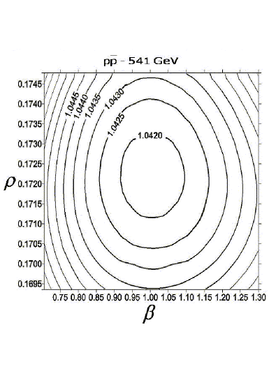
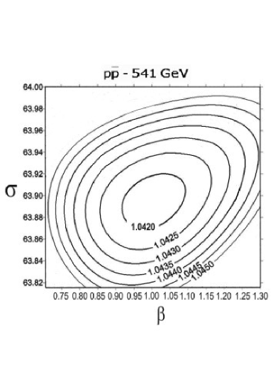
Figure 15: Correlations between the parameters $\rho$ and $\beta$ and between $\sigma$ and $\beta$ that lead to low values of $\chi^{2}$. In each case the other two parameters are let free while tables of $\chi^{2}$ are built with specified values for the two plotted parameters. Also the normalization factor 10.083 is taken as fixed independently from PAW fitting program.

We have built a file with a continuous and non superposing set of points, being the first 59 points from normalized dN/dt (with normalization factor 10.6) and 121 points from Bozzo et al. The 180 points form a regular $|t|$ distribution, which we fit with formulae from our previous work pereira_ferreira . The results are shown in Fig. 16.

Figure 16: Data at 541 GeV selected and organized. The dotted line is a fit described in our previous work pereira_ferreira .

The parameter values obtained in this fitting are $\sigma=~{}63.06\pm 1.90$ mb , $\rho=~{}0.124\pm 0.005$, $B_{I}=~{}13.88\pm 0.42~{}{\rm GeV}^{-2}$, $B_{R}=~{}25.79\pm 0.77~{}{\rm GeV}^{-2}$, with $\chi^{2}=1.32$.

III.8 p$\bar{\rm p}$ scattering at $\sqrt{s}$ = 1800 GeV

Two independent experiments, both at Fermilab, measured $d\sigma/dt$ for small $|t|$ at 1800 GeV, with a discrepancy of about 10 percent in the normalization for the total cross section. This is shown in Fig. 17.

Figure 17: Data and results at 1800 GeV .

Our determination of parameters (with fixed $\rho=0.14$) is given in Table 4. Although this is not a close determination, due to large variation bars, it is interesting that the lowest $\chi^{2}$ are obtained with $B_{R}$ larger than $B_{I}$, for both experiments..

Table 4: Forward scattering parameters at 1800 GeV

Experiment	$\sigma({\rm mb})$	$\rho$	$B_{I}({\rm GeV}^{-2})$	$B_{R}({\rm GeV}^{-2})$	$\chi^{2}$
E710	$72.748\pm 0.186$	$0.14$ (fixed)	$16.297\pm 0.039$	$115.57\pm 164.20$	$0.6020$
E710	$71.824\pm 0.184$	$0.14$ (fixed)	$16.282\pm 0.039$	$~{}B_{I}~{}({\rm fixed})$	$0.6060$
E710	$72.651\pm 0.186$	$1.0$ (fixed)	$16.284\pm 0.039$	$167.93\pm 48.561$	$0.5961$
CDF	$80.917\pm 0.436$	$0.14$(fixed)	$16.988\pm 0.087$	$72.006\pm 116.15$	$1.771$
CDF	$79.982\pm 0.432$	$0.14$(fixed)	$16.981\pm 0.087$	$B_{I}~{}({\rm fixed})$	$1.775$
CDF	$80.159\pm 0.433$	$1.0$(fixed)	$16.865\pm 0.087$	$85.730\pm 16.937$	$1.705$

From the results shown in Table 4, with large differences in $\chi^{2}$ values, we learn that the data from the E710 experiment are more compatible with the forward scattering basic expression (17) for $d\sigma/dt$ than the CDF data. Another important observed result is that increasing simultaneously the values $\rho$ and $B_{R}$ we may obtain the same, or lower, $\chi^{2}$ : the real amplitude at $|t|=0$ may be larger, but it decreases faster. It is as if for a given dataset we should keep constant a product $\rho e^{-(B_{R}/2)|t|_{\rm eff}}$ , with a value $|t|_{\rm eff}$ that is effective for the Coulomb interference region. For the E710 data we extract from the table that $|t|_{\rm eff}\approx 0.075$ ; for the CDF basis the value is rather large $|t|_{\rm eff}\approx 0.28$ . We thus see that the values of $\rho$ and $B_{R}$ at 1800 GeV are not determined from the existing data in this analysis.

The Fermilab data on $d\sigma/dt$ at 1.96 TeV are now launched in preliminary form, covering the $t|$ range from 0.26 to 1.30 $\nobreak\,\mbox{GeV}^{2}$. In Fig. 18 we show these new data together with the old 1.8 TeV data. The LHS plot gives also the lines representing the fittings of the E710 data (dashed line) and of the CDF data (dotted line) as informed in Table 4, with fixed $\rho=0.14$.

Figure 18: Data on p$\bar{\rm p}$ scattering at 1.8 and (preliminary) at 1.96 TeV. The lines in the LHS plot represent the fittings with the basic expression (17) : dashed for E710 and dotted line for CDF data. The RHS plot shows the fitting (solid line) of all the data (dashed line) with parameterization used in our previous work pereira_ferreira .

The RHS figure shows the fitting (solid line) of all these data (marked by the interpolating dashed line) using our previous parameterization expressions pereira_ferreira . We obtain $\chi^{2}=1.675$ for the whole lot of data (51+26+27=104 points). Taking only the E710 points together with the 1.96 TeV data (51+27=78 points) we obtain a beautiful representation with $\chi^{2}=0.45$; taking the CDF points together with the new 1.96 data (26+27=53 points) we obtain $\chi^{2}=0.74$. These results, that depend on our particular parameterization, but are meaningful because they come from a search for continuity in the data, again seem to favor the $t$ dependence and normalization of the E710 data.

III.9 Amplitudes

The lines representing $d\sigma/dt$ in Figs. 16 and 18 are obtained from real and imaginary amplitudes that are shown in Fig. 19, with their characteristic slopes and zeros .

Figure 19: Amplitudes of p$\bar{\rm p}$ scattering at 541 and 1800 (including preliminary 1960) GeV normalized to 1 at $|t|=0$. The amplitudes are obtained with parameterization used in previous work pereira_ferreira . Notice the linear scale in the LHS plot. The zeros of the real and imaginary amplitudes at 1800/1960 GeV occur respectively at about 0.05 and 0.68 $\nobreak\,\mbox{GeV}^{2}$ .

Some typical values of parameters obtained in this analysis of the full $t$ dependence, that can be read off from the plots of the amplitudes, are given in Table 5. These are possible, but not unique or necessarily correct, representations of the data.

Table 5: Quantities extracted from the $t$ dependence of the amplitudes at 541/546 and 1800/1960 GeV. Remarks: (1)Abe+Amos+1.96  ;  (2) Amos+1.96  ;   (3) Abe+1.96  .

$\sqrt{s}$	$\sigma$	$\rho$	$B_{I}$	$B_{R}$	$|t_{0}^{R}|$	$|t_{0}^{I}|$	$\chi^{2}$
(GeV)	(mb)		$({\rm GeV}^{-2})$	$({\rm GeV}^{-2})$	$({\rm GeV}^{2})$	$({\rm GeV}^{2})$
541/546	63.05	0.12	13.88	25.79	0.16	0.85	1.32
1800/1960  (1)	73.98	1.17	15.50	85.43	0.05	0.69	1.68
1800/1960  (2)	73.95	0.75	15.47	84.12	0.05	0.69	0.45
1800/1960 (3)	88.49	1.21	17.94	61.43	0.05	0.69	0.74

The real amplitude shows a large slope and falls rapidly to zero at a value $|t_{0}^{R}|$ that is expected to approach the origin in the form pereira_ferreira

$$|t_{0}^{R}|=\frac{1}{A+B\log{s}}~{},$$ (22)

following Martin’s discussion about the first zero of the real amplitude Martin . Obviously, as $|t_{0}|$ approaches the origin, $B_{R}$ grows with the energy.

The numbers indicate much indetermination in this analysis of the old data. In particular, identification of the values of $\rho$ and $B_{R}$ seems to be difficult. Dispersion relations must be used as a guide towards the disentanglement, in particular with application of the derivative dispersion relations for slopes EF2007 . We recall that the energy dependence in the measurements is crucial for the good use of dispersion relations, and we hope that LHC will produce diffractive data at several energies ?

IV remarks and conclusions

We have performed a detailed analysis of the data on differential elastic cross-sections allowing for the freedom of different slopes for the real and imaginary amplitudes, namely $B_{R}\neq B_{I}$, for the data points obtained in the ISR/SPS(Cern) and Tevatron (Fermilab) experiments during the years 1960-1990. The principal conclusion of the present analysis is that different values of the slopes, in particular the possibility of $B_{R}>B_{I}$ in accordance with the expectations from Martin’s theorem [2] and from dispersion relations [1], are perfectly consistent within the present errors of experimental data.

Our investigation concerns the four quantities relevant for the elastic forward processes, namely, $\sigma,\rho,B_{R}$ and $B_{I}$. Studying the behavior of $\chi^{2}$ values near its minimum and statistically equivalent parameter ranges, we observe that the available data from Cern and from Fermilab for small $\left|t\right|$ at the energies $20-2000$ GeV are not sufficient for a precise determination of these four parameters. With real and imaginary amplitudes as independent quantities in the form $\alpha~{}e^{\beta t}$, the $\chi^{2}$ analysis clearly shows a strong correlation among the parameters, exhibiting a very large valley in $\chi^{2}$ surface in the parameter space. This in particular leaves large ambiguities in the determination for the weaker real part.

It is interesting to note that detailed behavior in the $\chi^{2}$ surface in the parameter space depends very much on the chosen data sets. For example, the minimum of $\chi^{2}$/degrees-of-freedom varies from 0.1 to 1.3 in different energies. On the other hand, the variation of $\chi^{2}$ for appreciable changes of some parameters is less than 0.1 percent, in general indicating that their precise determination is not possible within the existing experimental situation.

On the other hand, it is worthwhile to mention that, if we have sufficient number of data points in this region, we do not need the absolute normalization of the luminosity, since the Coulomb interference can determine correctly the absolute value of cross section as a free parameter, as was shown in this work for the 541 GeV case. Of course, this method requires that the low $\left|t\right|$ data be very accurate. It is interesting to note that tests of this of Coulomb interference method, introducing a new free normalization parameter into the data set, are found to be compatible in both E-710 and E-741 Fermilab data at $1800$ GeV, while the difference in the evaluation of the total cross section remains.

As mentioned before, the quantitative analysis for the disentaglement of the real and imaginary parts of complex amplitude at small $\left|t\right|$ cannot be made with confidence with the data available up to now. Tests of quantities like the position of the zero of the real amplitude are not safe in these conditions. Thus model independent values for the four parameters cannot be obtained accurately.

Usually, the models suited for pp dynamics aimed to cover an overall large $\left|t\right|$ region, with correct description of dip and tail in $d\sigma/dt$, are not sensitive enough to the details of the behavior of scattering amplitudes for very small $\left|t\right|$ . In this region, the behavior of the amplitude maybe very sensitive to specific dynamical influences of the non-pertubative QCD dynamics. In particular, the forward scattering amplitude is directly related with the proton structure, and intimately related with the parton distribution function at small $x$ and saturation problems.

As a complimentary study, we also performed the analysis of scattering amplitude for a larger $\left|t\right|$ domain as proposed in pereira_ferreira . We observe that such analysis, consistent with the general structure of the scattering amplitudes, such as positions of zeros and dips, clearly shows the necessity of the very distinct values of the slope parameters of real and imaginary amplitudes, corroborating with the results obtained here from the analysis in small $\left|t\right|$ regions. In terms of scattering amplitude, this different behaviors of real and imaginary part is crucial and will be fundamental to understand the mechanism of elastic scattering amplitude.

Of course, the separation of complex amplitudes will never be a very easy task only from the measured scattering experiments, and it will be unavoidable to make use of other theoretical tools, such as dispersion relations. Particular attention must be given to the development and application of dispersion relations for slope parameters [1]. The knowledge of the energy dependence is crucial for the application of these tools in practice, and it is extremely interesting if an energy scan program is also included in the first phase of the LHC operation of p+p collisions.

Although no new or better method has been introduced in the present work, our precise analysis has revealed the existence of correlations and related uncertainties of the behavior of the scattering amplitude at small $\left|t\right|$. For quantitative determinations, more precise and numerous data points are necessary.

We expect to have a different situation in the future experiments from RHIC and LHC, with much better statistics and accuracy in the measurements of scattering data in the Coulomb interference region, together with a systematic energy scan program.

V Appendix: The calculation of the Coulomb phase

Here we give details of the evaluation of the phase of West and Yennie given by eq. (11) in the case where we let $B_{R}\neq B_{I}$ .

After eq. (12) we define

$$G_{R}=\frac{c}{c+i}=\frac{c(c-i)}{c^{2}+1}$$

$$G_{I}=\frac{1}{c+i}=\frac{(c-i)}{c^{2}+1}~{},$$ (23)

and the integral in eq.(11) is written

$$\int_{-4p^{2}}^{0}\frac{dt^{\prime}}{|t^{\prime}-t|}\bigg{[}1-\frac{F^{N}(s,t^{\prime})}{F^{N}(s,t)}\bigg{]}$$ (24)

$$= G_{R}\int_{-4p^{2}}^{0}\frac{dt^{\prime}}{|t^{\prime}-t|}\bigg{[}1-e^{B_{R}(t^{\prime}-t)/2}\bigg{]}+iG_{I}\int_{-4p^{2}}^{0}\frac{dt^{\prime}}{|t^{\prime}-t|}\bigg{[}1-e^{B_{I}(t^{\prime}-t)/2}\bigg{]}~{},$$

and then

$$\Phi(s,t) = (-/+)\Bigg{[}\ln(-\frac{t}{s})+G_{R}\int_{-4p^{2}}^{0}\frac{dt^{\prime}}{|t^{\prime}-t|}\bigg{[}1-e^{B_{R}(t^{\prime}-t)/2}\bigg{]}$$ (25)

$$+ iG_{I}\int_{-4p^{2}}^{0}\frac{dt^{\prime}}{|t^{\prime}-t|}\bigg{[}1-e^{B_{I}(t^{\prime}-t)/2}\bigg{]}\Bigg{]}~{}.$$

We note that both integrals are of the form

$$I(B)=\int_{-4p^{2}}^{0}\frac{dt^{\prime}}{|t^{\prime}-t|}\bigg{[}1-e^{B(t^{\prime}-t)/2}\bigg{]}~{}$$ (26)

which has been studied by V. Kundrát and M. Lokajicek KL . With $x=t^{\prime}-t$ and $y=Bx/2$, we have

$$I(B) = \int_{-4p^{2}}^{0}\frac{dx}{|x|}\bigg{[}1-e^{Bx/2}\bigg{]}=\int_{-B(4p^{2}+t)/2}^{-Bt/2}\frac{dy}{|y|}\bigg{[}1-e^{y}\bigg{]}$$ (27)

$$= \int_{-B(4p^{2}+t)/2}^{0}\frac{dy}{|y|}\bigg{[}1-e^{y}\bigg{]}+\int_{0}^{-Bt/2}\frac{dy}{|y|}\bigg{[}1-e^{y}\bigg{]}$$

$$= \int_{0}^{B(4p^{2}+t)/2}\frac{dy}{|y|}\bigg{[}1-e^{-y}\bigg{]}-\int_{0}^{-Bt/2}\frac{dy}{|y|}\bigg{[}e^{y}-1\bigg{]}$$

These expressions can be written in terms of exponential integrals, as can be seen in the Handbook of Mathematical Functions of M. Abramowitz and L.A. Stegun abramowitz as

$$\int_{0}^{B(4p^{2}+t)/2}\frac{dy}{|y|}\bigg{[}1-e^{-y}\bigg{]}=E_{1}\bigg{[}\frac{B}{2}\bigg{(}4p^{2}+t\bigg{)}\bigg{]}+\ln\bigg{[}\frac{B}{2}\bigg{(}4p^{2}+t\bigg{)}\bigg{]}+\gamma$$ (28)

and

$$\int_{0}^{-Bt/2}\frac{dy}{|y|}\bigg{[}e^{y}-1\bigg{]}=E_{i}\bigg{(}-\frac{B}{2}t\bigg{)}-\ln\bigg{(}-\frac{B}{2}t\bigg{)}-\gamma$$ (29)

where $\gamma=0.5772$ is the Euler constant.

Thus the integrals that appear in eq. (24) have the functional form

$$I(B)=E_{1}\big{[}\frac{B}{2}\bigg{(}4p^{2}+t\bigg{)}\big{]}-E_{i}\big{[}-\frac{Bt}{2}\big{]}+\ln\big{[}\frac{B}{2}\bigg{(}4p^{2}+t\bigg{)}\big{]}-\ln\big{[}-\frac{Bt}{2}\big{]}+2\gamma~{},$$ (30)

and the phase can be written

$$\Phi(s,t)=(-/+)\Bigg{[}\ln\bigg{(}-\frac{t}{s}\bigg{)}+G_{R}~{}I(B_{R})+iG_{I}~{}I(B_{I})\Bigg{]}$$ (31)

or

$$\Phi(s,t)=(-/+)\Bigg{[}\ln\bigg{(}-\frac{t}{s}\bigg{)}+\frac{1}{c^{2}+1}\bigg{[}c^{2}I(B_{R})+I(B_{I})\bigg{]}+i\frac{c}{c^{2}+1}\bigg{[}I(B_{I})-I(B_{R})\bigg{]}\Bigg{]}~{}.$$ (32)

The real part of the phase is taken into eq. ( 5 ) .

References

- (1) R. Fiore, L. Jenkovszky, R. Orava, E. Predazzi, A. Produkin and O. Selyugin, emphhep-ph/0810.2902
- (2) E. Ferreira, Int. J. Mod. Phys. E 16, 2893 (2007)
- (3) A. Martin , Phys. Lett. B 404, 137 (1997)
- (4) P. Gauron, B. Nicolescu and O.V. Selyugin, Phys. Lett. B 629, 83 (2005)
- (5) G. B. West and D. Yennie , Phys. Rev. 172, 1413 (1968)
- (6) O. V. Selyugin , Mod. Phys. Lett. A 11, 2317 (1996); Mod. Phys. Lett. A 12, 1379 (1997); Phys. Rev. D 60, 074028 (1999)
- (7) V.A. Petrov, E. Predazzi and A. Prokudin, Eur. Phys. J. C 28, 525 (2003)
- (8) V.Kundrát and M.Lokajicek, Phys. Lett. B 611, 102 (2005)
- (9) M. Abramowitz and I. Stegun, Handbook of Mathematical Functions , Dover, New York, 1972
- (10) J.R.Cudell, A. Lengyel and E. Martynov, Phys. Rev. D 73, 034008 (2006) [hep-ph/0511073]
- (11) U. Amaldi and K. R. Schubert , Nucl. Phys. B 166, 301 (1980)
- (12) A. A. Kuznetsov et al. , Sov. J. Nucl. Phys. 33, 74 (1981), and Yad. Fiz. 33, 142 (1981)
- (13) A. Schiz et al. , exp. FNAL-069A , Phys. Rev. D 24, 26 1981
- (14) N. A. Amos et al., Nucl. Phys. B 262, 689 (1985)
- (15) F. Pereira and E. Ferreira, Phys. Rev. D 59, 014008 (1999) ; Phys. Rev. D 61, 077507 (2000) Int. J. Mod. Phys. E 16, 2889 (2007)
- (16) C. Augier et al. , CERN UA4/2 Coll. , Phys. Lett. B 316, 448 (1993)
- (17) G. Arnison et al. , CERN UA1 Coll. , Phys. Lett. B 128, 336 (1983)
- (18) M. Bozzo et al., CERN UA4 Coll., Phys. Lett. B 147, 385 (1984)
- (19) M. Bozzo et al., CERN UA4 Coll., Phys. Lett. B 155, 197 (1985)
- (20) D. Bernard et al., CERN UA4 Coll., Phys. Lett. B 198, 583 (1987)
- (21) F. Abe , Fermilab CDF Coll., Phys. Rev. D 50, 5518 (1993)