Itinerant ferromagnetism in an atomic Fermi gas: Influence of population imbalance

Abstract

We investigate ferromagnetic ordering in an itinerant ultracold atomic Fermi gas with repulsive interactions and population imbalance. In a spatially uniform system, we show that at zero temperature the transition to the itinerant magnetic phase transforms from first to second order with increasing population imbalance. Drawing on these results, we elucidate the phases present in a trapped geometry, finding three characteristic types of behavior with changing population imbalance. Finally, we outline the potential experimental implications of the findings.

I Introduction

Feshbach resonance phenomena provide unprecedented control of pair interactions in degenerate atomic Fermi gases Stwalley (1976); Tiesinga et al. (1993). This feature has allowed extensive studies of pairing phenomena in two-component Fermi gases providing access to the crossover between a Bose-Einstein condensate (BEC) of molecules and the Bardeen-Cooper-Schrieffer (BCS) state of Cooper pairs Strecker et al. (2003); Gupta et al. (2003); Chin et al. (2004); Regal et al. (2004). Although the emphasis of experimental investigations has been primarily on the problem of resonance superfluidity, interacting Fermi gases support other strongly-correlated phases including itinerant ferromagnetism.

In solid state condensed matter systems, the problem of itinerant ferromagnetism has a long history dating back to the pioneering studies by Stoner Stoner (1937) and Wohlfarth Wohlfarth and Rhodes (1962). These early investigations proposed that, at low enough temperatures, a Fermi gas subject to a repulsive interaction potential could undergo a continuous phase transition into an itinerant spin polarized phase Ziman (1979). This Stoner transition reflects the shifting balance between the potential energy gained in spin polarization through Pauli exclusion statistics, and the associated cost in kinetic energy. Subsequent studies showed that fluctuations in the magnetization at low temperatures drive the second order transition first order at low enough temperatures Shimizu (1964); Belitz et al. (1997, 1999); Vojta (2000); Belitz and Kirkpatrick (2002); Belitz et al. (2005). Such behavior is born out around quantum criticality in a variety of experimental solid state systems including $\text{ZrZn}_{2}$ Uhlarz et al. (2004, 2005), $\text{UGe}_{2}$ Huxley et al. (2000), MnSi Pfleiderer et al. (2001); Yu et al. (2004); Uemura et al. (2007); Otero-Leal et al. (2009); Petrova et al. (2009), $\text{CoS}_{2}$ Otero-Leal et al. (2008), $\text{YbRh}_{2}\text{Si}_{2}$ Misawa et al. (2008), and $\text{SrRuO}_{3}$ Hamlin et al. (2007). When subject to a magnetic field, the attendant increase in Zeeman energy results in the bifurcation of the tricritical point separating the region of first and second order ferromagnetic transitions into two lines of metamagnetic critical points.

In the following, we will explore the potential implications of this itinerant magnetic phase behavior on the equilibrium properties of strongly interacting two-component atomic Fermi gases; here we refer to the pseudo-spin associated with the hyperfine states characterizing the two atomic populations. However, in contrast to the solid state system, the application of these ideas to the atomic Fermi gas must address the features imposed by the trap geometry, and the constraints resulting from the inability of particles to transfer between different spin states Liu and Hui (2006). As a result, in the general case, one must consider atomic Fermi mixtures in which an effective spin polarization is imposed by population imbalance Combescot (2007); Sheehy and Radzihovsky (2007a). The potential for itinerant ferromagnetism in atomic Fermi gases has been already addressed in the literature, Zhang et al. (2008) showed that an optical lattice would reduce the repulsive interaction strength required to realize ferromagnetism, and Sogo and Yabu (2002) studied a trapped system in the Thomas-Fermi approximation. Subsequently, Duine and MacDonald (2005) developed a diagrammatic perturbative expansion in interaction strength to address the phase behavior of the balanced two-component Fermi system. In the following, we will develop a functional integral formulation to explore the phase behavior of the general population imbalanced system. As well as providing access to the mean-field phase behavior of the system, such an approach allows for future considerations of the collective low energy spin dynamics of the spin polarized phase. Moreover, the theory provides a platform to explore the potential for the development of an equilibrium spin textured phase recently conjectured in relation to the solid state system Belitz et al. (1997); Huxley et al. (2001); Watanabe and Miyake (2002); Kitagawa et al. (2005); Berdnikov et al. (2008).

The paper is organized as follows: In Sec. II we derive an expression for the thermodynamic potential of the system as a function of the local density and in-plane magnetization fields. To address the important effects of spin-wave fluctuations on the nature of the equilibrium phase diagram, we will explore the renormalization of the mean-field equations keeping those terms that are second order in the coupling strength, $g$. Using this result, in Sec. III.1 we analyze the phase diagram of the spatially uniform system as a function of the interaction strength, $g$, and chemical potential shift. Finally, in Sec. III.2 we explore in detail the phase behavior of the magnetic system in the atomic trap geometry.

II Field integral formulation

Expressed as a coherent state path integral, the quantum partition function of a population imbalanced two-component Fermi gas is given by

$$\mathcal{Z} = \int\!\!\mathcal{D}\psi\exp\Biggl{[}-\int_{0}^{\beta}\!\!d\tau\,d\mathbf{r}\!\!\!\!\sum_{\sigma=\{\uparrow,\downarrow\}}\!\!\!\!\bar{\psi}_{\sigma}(-\text{i}\partial_{\tau}+\hat{\xi}-\sigma\Delta\mu)\psi_{\sigma}$$ (1)

$$- \int_{0}^{\beta}d\tau\,d\mathbf{r}\,g\bar{\psi}_{\uparrow}\bar{\psi}_{\downarrow}\psi_{\downarrow}\psi_{\uparrow}\Biggr{]}\,.$$

where $\bar{\psi}_{\sigma}(\tau,\mathbf{r})$ and $\psi_{\sigma}(\tau,\mathbf{r})$ denote Grassmann fields, $\beta=1/k_{\rm B}T$ is the inverse temperature, and $\hat{\xi}=\hat{p}^{2}/2m-\mu$. Here we have used a pseudo-spin index, $\sigma\in\{\uparrow,\downarrow\}$, to discriminate the two components. As independent particles (with no interconversion), the density of the two majority/minority degrees of freedom must be specified by two chemical potentials. For convenience, it is helpful to separate the chemical potentials into their sum and difference; $\mu+\Delta\mu$ for up-spin and $\mu-\Delta\mu$ for down-spin. In this representation, population imbalance may be adjusted through the chemical potential shift, $\Delta\mu$. Note that, although population imbalance is synonymous with a global pseudo-spin magnetization, a spontaneous symmetry breaking into an itinerant ferromagnetic phase can still develop with the appearance of a non-zero in-plane component of the magnetization. Finally, we suppose that the strength of the repulsive $s$-wave contact interaction, $g\delta^{3}(\mathbf{r})$, can be tuned using a Feshbach resonance.

II.1 Hubbard-Stratonovich decoupling

To develop an effective low-energy theory for the Fermi gas, it is convenient to decouple the quartic contact interaction by introducing auxiliary bosonic fields, $\rho$ and ${\bm{\phi}}$, conjugate to the local density $\sum_{\alpha=\{\uparrow,\downarrow\}}\bar{\psi}_{\alpha}\psi_{\alpha}$ and magnetization $\sum_{\alpha,\beta=\{\uparrow,\downarrow\}}\bar{\psi}_{\alpha}{\bm{\sigma}}_{\alpha\beta}\psi_{\beta}$ respectively, setting

$$\mathcal{Z} =\int\mathcal{D}{\bm{\phi}}\mathcal{D}\rho\mathcal{D}\psi\exp\Biggl{\{}-\int d\tau d\mathbf{r}\,\Biggl{[}g({\bm{\phi}}^{2}-\rho^{2})$$

$$+ \!\!\!\!\!\!\!\!\sum_{\alpha,\beta=\{\uparrow,\downarrow\}}\!\!\!\!\!\!\bar{\psi}_{\alpha}\left[(\hat{G}_{0}^{-1}+g\rho)\delta_{\alpha\beta}-(\Delta\mu\mathbf{e}_{\text{z}}+g{\bm{\phi}})\cdot{\bm{\sigma}}_{\alpha\beta}\right]\psi_{\beta}\Biggr{]}\!\Biggr{\}}.$$

Here $\hat{G}_{0}=(-\text{i}\partial_{t}+\hat{\xi})^{-1}$ defines the Green’s function of the non-interacting system, and ${\bm{\sigma}}$ denotes the vector of Pauli spin matrices. Note that, without decoupling in both the Hartree and Fock channels, one would subsequently encounter unphysical diagrammatic contributions to the perturbative scheme developed below Keiter (1970); Evenson et al. (1970); Morandi et al. (1974). It is also the simplest approach that maintains spin rotational invariance of the Hamiltonian, and leads to the correct set of Hartree-Fock equations Hubbard (1979); Prange and Korenman (1979a). Then, integrating over the Fermi fields, one obtains the expression

$$\mathcal{Z}=\int\mathcal{D}{\bm{\phi}}\mathcal{D}\rho\mathcal{D}\psi\,\text{e}^{{-\int d\tau d\mathbf{r}\,g({\bm{\phi}}^{2}-\rho^{2})}}$$

$$\times\exp\left[\operatorname{Tr}\ln\left(\hat{G}_{0}^{-1}+g\rho-{\bm{\sigma}}\cdot\left(\Delta\mu\mathbf{e}_{\text{z}}+g{\bm{\phi}}\right)\right)\right]\,.$$ (3)

At this stage the analysis is exact, but to proceed further one must employ an approximation. To orient our discussion and make contact with conventional Stoner theory, let us first consider a direct saddle-point approximation scheme.

II.2 Stoner mean-field theory

As well as the “effective” magnetization imposed by population imbalance, we anticipate the development of a spontaneous magnetization which will drive the axis of quantization away from the z-axis. We re-orient the axis of quantization to lie parallel to the net magnetization, denoted in mean-field theory (with over-bars) $\overline{{\bm{\phi}}}=\overline{{\bm{\phi}}}_{\perp}+\overline{\phi}_{\text{z}}\mathbf{e}_{\text{z}}$, $\overline{{\bm{\phi}}}_{\perp}=(\overline{\phi}_{\text{x}},\overline{\phi}_{\text{y}})$, and with this definition, the total magnetization of the system is given by $\overline{\mathbf{M}}=\Delta\mu\mathbf{e}_{\text{z}}/g+\overline{{\bm{\phi}}}$. Separately varying the action with respect to $\overline{{\bm{\phi}}}_{\perp}$ and $\overline{\phi}_{\text{z}}$ one obtains, respectively, the saddle-point equations,

$$\left(\begin{array}[]{c}\overline{{\bm{\phi}}}_{\perp}\\ \overline{\phi}_{\text{z}}\end{array}\right)=-\frac{(\beta V)^{-1}\operatorname{Tr}(\hat{G}_{+}-\hat{G}_{-})}{\sqrt{(g\overline{{\bm{\phi}}}_{\perp})^{2}+(g\overline{\phi}_{\text{z}}+\Delta\mu)^{2}}}\left(\begin{array}[]{c}g\overline{{\bm{\phi}}}_{\perp}\\ g\overline{\phi}_{\text{z}}+\Delta\mu\end{array}\right)\,,$$

where $\hat{G}_{\pm}^{-1}=\hat{G}_{0}^{-1}+g\overline{\rho}\mp\left|\Delta\mu\mathbf{e}_{\text{z}}+g\overline{{\bm{\phi}}}\right|$, and $V$ denotes the total volume of the system. Together, these equations admit two possible solutions:

[$\overline{{\bm{\phi}}}_{\perp}=\mathbf{0}$ and $\overline{M}=\overline{\phi}_{\text{{z}}}$]:

The total magnetization of the system can be ascribed to population imbalance with no spontaneous magnetization in-plane. Within this solution, $\overline{M}$ is a function of $|g\overline{\phi}_{\text{z}}+\Delta\mu|$, so it can be used to infer the chemical potential shift, $\Delta\mu$.

[$\overline{{\bm{\phi}}}_{\perp}\neq\mathbf{0}$]:

The total magnetization takes the form $\overline{M}=(\overline{{\bm{\phi}}}_{\perp}^{2}+\overline{\phi}_{\text{z}}^{2})^{1/2}$. Along z-axis, the magnetization is fixed due to population imbalance, with the additional magnetization developing within the x-y plane. In this case, the saddle-point solution translates to the condition $\Delta\mu=0$, i.e. no chemical potential shift is required to recover the fixed z-component of the magnetization due to the population imbalance; it is simply given by the resolved component of the total magnetization.

The total population $N=N_{\uparrow}+N_{\downarrow}$ can in turn be obtained from the variation $\delta\overline{S}/\delta\overline{\rho}=0$.

Expanding the action in interaction strength, $g$, $\overline{S}=g\phi_{\text{z}}^{2}\operatorname{Tr}(1+g\hat{G}_{0}\hat{G}_{0})=g\phi_{\text{z}}^{2}(1-g\nu)$, and one can extract the familiar Stoner criterion Kanamori (1963); Hubbard (1963) for a population balanced system, with $\nu$ being the density of states. For $g\nu<1$ the state is unmagnetized, $\overline{M}=0$, and chemical potentials of the two Fermi surfaces remain equal. If $g\nu>1$ then the state is magnetized with $\overline{M}=\sqrt{(g\nu-1)/g^{3}\nu^{\prime\prime}}$. We also note that the Stoner criterion can be reformulated to account for population imbalance giving $\overline{S}=g\phi^{2}(1-g\nu)-g^{2}\Delta\mu^{2}$, leading to a transition at the same value of interaction strength as for the balanced system. Although, at this order, the saddle-point approximation predicts a continuous transition to a ferromagnetic phase for the balanced system, it is well-established that fluctuations of the magnetization field drive the transition first order at low temperature Abrikosov and Khalatnikov (1958). This effect can be captured by retaining fluctuation contributions to second order in the interaction. In the following, we will explore the impact of fluctuations on the equations of motion associated with the uniform mean-field.

II.3 Integrating out auxiliary field fluctuations

To implement this program, it is convenient to parameterize the Hubbard-Stratonovich fields into some, as yet undetermined, stationary (spatially uniform) values ${\bm{\phi}}_{0}$ and $\rho_{0}$, and fluctuations around them, ${\bm{\phi}}_{\text{fl}}$ and $\rho_{\text{fl}}$. Integrating out these fluctuations, the goal is to obtain the renormalized mean-field equations for ${\bm{\phi}}_{0}$ and $\rho_{0}$ retaining contributions to second order in $g$. Substituting ${\bm{\phi}}={\bm{\phi}}_{0}+{\bm{\phi}}_{\text{fl}}$ and $\rho=\rho_{0}+\rho_{\text{fl}}$ into Eq. (3), and rotating the z-axis from the quantization direction to lie along the direction of uniform magnetization using the constant matrix $\mathsf{T}$, one obtains

$$\mathcal{Z} \!\!=\text{e}^{{-\beta Vg({\bm{\phi}}_{0}^{2}-\rho_{0}^{2})}}\!\!\int\!\!\mathcal{D}\rho_{\text{fl}}\mathcal{D}{\bm{\phi}}_{\text{fl}}\,\exp{\left[-\!\!\int\!\!d\tau d\mathbf{r}\,g({\bm{\phi}}_{\text{fl}}^{2}-\rho_{\text{fl}}^{2})\right]}$$

$$\times \!\!\exp\left[\operatorname{Tr}\ln\mathsf{G}^{-1}+\operatorname{Tr}\ln(\mathsf{I}+g\mathsf{G}\mathsf{T}^{-1}(\mathsf{I}\rho_{\text{fl}}+{\bm{\sigma}}\cdot{\bm{\phi}}_{\text{fl}})\mathsf{T})\right]\,,$$

where now $\hat{G}_{\pm}^{-1}=\hat{G}_{0}^{-1}+g\rho_{0}\mp|\Delta\mu\mathbf{e}_{\text{z}}+g{\bm{\phi}}_{0}|$ denotes the elements of the inverse Green’s function of the system at the level of the renormalized mean-field, $\mathsf{\hat{G}}={\rm diag}(\hat{G}_{+},\hat{G}_{-})$. Then, expanding the action to second order in fluctuations, $\rho_{\text{fl}}(\mathbf{r},\tau)$ and ${\bm{\phi}}_{\text{fl}}(\mathbf{r},\tau)$, and performing the functional integral, one obtains the thermodynamic grand potential from the quantum partition function using $\Phi_{\text{G}}=-\beta^{-1}\ln\mathcal{Z}$,

$$\Phi_{\text{G}}=\overbrace{\operatorname{Tr}\ln\hat{G}_{+}^{-1}+\operatorname{Tr}\ln\hat{G}_{-}^{-1}}^{\displaystyle{\dagger}}+g\left(\phi_{0}^{2}-\rho_{0}^{2}\right)$$

$$+\overbrace{\frac{1}{2}\operatorname{Tr}\ln\left(1-g^{2}\Pi_{++}\Pi_{--}\right)}^{\displaystyle{\parallel}}$$

$$+\overbrace{\frac{1}{2}\operatorname{Tr}\ln\left(1+g\Pi_{+-}+g\Pi_{-+}+g^{2}\Pi_{+-}\Pi_{-+}\right)}^{\displaystyle{\perp}}\,,$$ (4)

a result that is independent of the transformation $\mathsf{T}$. Here we have defined the spin-dependent polarization operator,

$$\Pi_{ss^{\prime}}(\omega,\mathbf{q})=\frac{2}{\beta V}\sum_{\omega^{\prime},\mathbf{k}}G_{s}(\omega^{\prime},\mathbf{k})G_{s^{\prime}}(\omega^{\prime}-\omega,\mathbf{k}-\mathbf{q})\,,$$

where the sum on $\omega^{\prime}$ runs over fermionic Matsubara frequencies. The term labeled ($\dagger$) simply represents the thermodynamic potential of a non-interacting Fermi gas with shifted chemical potentials. The term labeled ($\perp$) is due to transverse fluctuations of the magnetization field and coincides with that obtained in Ref. Prange and Korenman (1979b). By contrast, the term labeled ($\parallel$), corresponding to longitudinal fluctuations, differs from that obtained in Ref. Prange and Korenman (1979b) by the additional contributions from density fluctuation effects.

To proceed, we now expand the potential $\Phi_{\text{G}}$ to second order in $g$ and perform the summations over Matsubara frequencies. Rearranging the momenta summations, one obtains

$$\Phi_{\text{G}} =-\frac{1}{\beta V}\sum_{\begin{subarray}{c}{\mathbf{k}}\\ {s=\{+,-\}}\end{subarray}}\ln\left(1+\text{e}^{-\beta(\epsilon_{\mathbf{k}}-\mu_{s})}\right)$$

$$+ g\left({\bm{\phi}}_{0}^{2}-\rho_{0}^{2}\right)+gN_{+}N_{-}$$

$$+ \!\!\frac{2g^{2}}{V}\!\!\sum_{\mathbf{k}_{1,2,3}}\!\!\frac{\overbrace{n_{+}(\epsilon_{\mathbf{k}_{1}})n_{-}(\epsilon_{\mathbf{k}_{2}})}^{\displaystyle{\Diamond}}(1\!-\!n_{+}(\epsilon_{\mathbf{k}_{3}}))(1\!-\!n_{-}(\epsilon_{\mathbf{k}_{4}}))}{\epsilon_{\mathbf{k}_{1}}+\epsilon_{\mathbf{k}_{2}}-\epsilon_{\mathbf{k}_{3}}-\epsilon_{\mathbf{k}_{4}}}\,,$$

where $\mu_{s}=\mu-g\rho_{0}+s|\Delta\mu\mathbf{e}_{\text{z}}+g{\bm{\phi}}_{0}|$, $n_{s}(\epsilon)=(1+\exp(-\beta(\epsilon-\mu_{s})))^{-1}$, and $N_{s}=\sum_{\mathbf{k}}n_{s}(\epsilon_{\mathbf{k}})$. Conservation of momentum requires that $\mathbf{k}_{1}+\mathbf{k}_{2}=\mathbf{k}_{3}+\mathbf{k}_{4}$. Physically, the numerator of the second order term indicates that the matrix element associated with the transition $(\mathbf{k}_{1},\mathbf{k}_{2})\rightarrow(\mathbf{k}_{3},\mathbf{k}_{4})$ is proportional to the probability that states $\mathbf{k}_{1}$ and $\mathbf{k}_{2}$ are occupied, whilst states $\mathbf{k}_{3}$ and $\mathbf{k}_{4}$ are unoccupied. Following Pathria (1996) (and the earlier discussion of Abrikosov and Khalatnikov (1958)), to renormalize the unphysical divergence of the term in $n^{2}(\epsilon)$, labeled ($\Diamond$) close to resonance, we regularize the effective interaction at second order in scattering length $a$,

$$g(\mathbf{k}_{1},\mathbf{k}_{2})\mapsto\frac{2k_{\text{F}}a}{\pi\nu}-\frac{8k_{\text{F}}^{2}a^{2}}{\pi^{2}\nu^{2}V^{2}}\sum_{\mathbf{k}_{3,4}}\frac{1}{\epsilon_{\mathbf{k}_{1}}+\epsilon_{\mathbf{k}_{2}}-\epsilon_{\mathbf{k}_{3}}-\epsilon_{\mathbf{k}_{4}}}\,,$$

where $\nu=\sqrt{\mu}/\sqrt{2}\pi^{2}$ and $k_{\text{F}}=\sqrt{2m\mu}$. In a population imbalanced system the definition for the chemical potential is that which gives the same total number of particles in the population balanced system, that is $k_{\text{F}}=\sqrt[3]{3\pi^{2}(n_{\uparrow}+n_{\downarrow})}$, where $n_{\uparrow}$ and $n_{\downarrow}$ are the number of up and down-spin particles; this definition holds true in both the canonical and grand canonical ensembles. This regularization of the contact interaction exactly cancels the divergent terms in $n^{2}(\epsilon)$, labeled ($\Diamond$). Furthermore, the terms in $n^{4}(\epsilon)$ are zero by symmetry. Finally, making use of the symmetry in $\mathbf{k}_{3}$ and $\mathbf{k}_{4}$, one obtains

$$\Phi_{\text{G}} =-\frac{1}{\beta V}\sum_{\begin{subarray}{c}{\mathbf{k}}\\ {s=\{+,-\}}\end{subarray}}\ln\left(1+\text{e}^{-\beta(\epsilon_{\mathbf{k}}-\mu_{s})}\right)$$

$$+ \!\!\!\!\frac{2k_{\text{F}}a}{\pi\nu}\left({\bm{\phi}}_{0}^{2}-\rho_{0}^{2}\right)+\frac{2k_{\text{F}}a}{\pi\nu}N_{+}N_{-}$$

$$- \!\!\!\!\frac{8k_{\text{F}}^{2}a^{2}}{\pi^{2}\nu^{2}V^{3}}\sum_{\mathbf{k}_{1,2,3}}\frac{n_{+}(\epsilon_{\mathbf{k}_{1}})n_{-}(\epsilon_{\mathbf{k}_{2}})\left(n_{+}(\epsilon_{\mathbf{k}_{3}})+n_{-}(\epsilon_{\mathbf{k}_{3}})\right)}{\epsilon_{\mathbf{k}_{1}}+\epsilon_{\mathbf{k}_{2}}-\epsilon_{\mathbf{k}_{3}}-\epsilon_{\mathbf{k}_{4}}}\,.$$

From the thermodynamic potential we can compute the free energy per unit volume $F=\Phi_{\text{G}}+\sum_{\sigma=\{\uparrow,\downarrow\}}(\mu+\sigma\Delta\mu)N_{\sigma}$. To consolidate terms entering the free energy we switch from the population imbalance pseudo-spin basis to the magnetization basis, retain contributions to order ${\cal O}((k_{\text{F}}a)^{2})$, recall that if $\Delta\mu=0$ then $M\neq 0$, whereas if $\Delta\mu\neq 0$ then $M=0$, and affect the rearrangement

$$\frac{2k_{\text{F}}a}{\pi\nu}\left({\bm{\phi}}_{0}^{2}-\rho_{0}^{2}\right)+\sum_{\sigma=\{\uparrow,\downarrow\}}(\mu+\sigma\Delta\mu)N_{\sigma}$$

$$=\overbrace{\left(\mu-\frac{2k_{\text{F}}a}{\pi\nu}\rho_{0}+\left|\Delta\mu\mathbf{e}_{\text{z}}+\frac{2k_{\text{F}}a}{\pi\nu}{\bm{\phi}}_{0}\right|\right)}^{\displaystyle{\mu_{+}}}N_{+}+\overbrace{\left(\mu-\frac{2k_{\text{F}}a}{\pi\nu}\rho_{0}-\left|\Delta\mu\mathbf{e}_{\text{z}}+\frac{2k_{\text{F}}a}{\pi\nu}{\bm{\phi}}_{0}\right|\right)}^{\displaystyle{\mu_{-}}}N_{-}$$

$$\left.{\begin{array}[]{l}+\frac{2k_{\text{F}}a}{\pi\nu}\left({\bm{\phi}}_{0}^{2}-\rho_{0}^{2}\right)+\left(\frac{2k_{\text{F}}a}{\pi\nu}\rho_{0}+\Delta\mu-\left|\Delta\mu\mathbf{e}_{\text{z}}+\frac{2k_{\text{F}}a}{\pi\nu}{\bm{\phi}}_{0}\right|\right)N_{+}\\ +\left(\frac{2k_{\text{F}}a}{\pi\nu}\rho_{0}-\Delta\mu+\left|\Delta\mu\mathbf{e}_{\text{z}}+\frac{2k_{\text{F}}a}{\pi\nu}{\bm{\phi}}_{0}\right|\right)N_{-}\end{array}}\right\}{\varnothing}\,.$$

Then, if we set ${\bm{\phi}}_{0}=\overline{{\bm{\phi}}}+\Delta{\bm{\phi}}$ and $\rho_{0}=\overline{\rho}+\Delta\rho$, an expansion in $\Delta{\bm{\phi}}$ and $\Delta\rho$ shows that the terms labeled ($\varnothing$) sum to zero to the accuracy of the free energy, $\mathcal{O}((k_{\text{F}}a)^{2})$. Retaining the remaining contribution, the free energy reduces to the form,

$$\!\!\!\!F \!\!\!=\!\overbrace{-\frac{1}{\beta V}\!\!\!\!\!\!\sum_{\begin{subarray}{c}{\mathbf{k}}\\ {s=\{+,-\}}\end{subarray}}\!\!\!\!\!\!\ln\left(\!1\!+\!\text{e}^{-\beta(\epsilon_{\mathbf{k}}-\mu_{s})}\!\right)\!+\!\!\!\!\!\!\sum_{s=\{+,-\}}\!\!\!\!\mu_{s}N_{s}}^{\displaystyle{\ddagger}}+\frac{2k_{\text{F}}a}{\pi\nu}N_{+}N_{-}$$

$$\!\!\!\!- \frac{8k_{\text{F}}^{2}a^{2}}{\pi^{2}\nu^{2}V^{3}}\sum_{\mathbf{k}_{1,2,3}}\!\frac{n_{+}(\epsilon_{\mathbf{k}_{1}})n_{-}(\epsilon_{\mathbf{k}_{2}})\left(n_{+}(\epsilon_{\mathbf{k}_{3}})+n_{-}(\epsilon_{\mathbf{k}_{3}})\right)}{\epsilon_{\mathbf{k}_{1}}+\epsilon_{\mathbf{k}_{2}}-\epsilon_{\mathbf{k}_{3}}-\epsilon_{\mathbf{k}_{4}}}\,.$$

This expression coincides with that obtained in Ref. Duine and MacDonald (2005). The method employed in the numerical calculation of the summation over three momenta is described in App. A.

II.4 Magnetization

To minimize the free energy and obtain the net magnetization it is convenient to take the expression for the thermodynamic potential (II.3) and affect the shift of the field $\Phi_{\text{z}}\mapsto\Phi_{\text{z}}-\Delta\mu\pi\nu/2k_{\text{F}a}$. As a result, the thermodynamic potential takes the form

$$\Phi_{\text{G}} =-\frac{1}{\beta V}\sum_{\begin{subarray}{c}{\mathbf{k}}\\ {s=\{+,-\}}\end{subarray}}\ln\left(1+\text{e}^{-\beta(\epsilon_{\mathbf{k}}-\mu_{s})}\right)$$

$$+ \!\!\frac{2k_{\text{F}}a}{\pi\nu}\left|{\bm{\phi}}_{0}-\frac{\Delta\mu\mathbf{e}_{\text{z}}\pi\nu}{2k_{\text{F}a}}\right|^{2}-\frac{2k_{\text{F}}a}{\pi\nu}\rho_{0}^{2}+\frac{2k_{\text{F}}a}{\pi\nu}N_{+}N_{-}$$

$$- \!\!\frac{8k_{\text{F}}^{2}a^{2}}{\pi^{2}\nu^{2}V^{3}}\sum_{\mathbf{k}_{1,2,3}}\frac{n_{+}(\epsilon_{\mathbf{k}_{1}})n_{-}(\epsilon_{\mathbf{k}_{2}})\left(n_{+}(\epsilon_{\mathbf{k}_{3}})+n_{-}(\epsilon_{\mathbf{k}_{3}})\right)}{\epsilon_{\mathbf{k}_{1}}+\epsilon_{\mathbf{k}_{2}}-\epsilon_{\mathbf{k}_{3}}-\epsilon_{\mathbf{k}_{4}}}\,,$$

where, in response to the shift of $\Phi_{\text{z}}$, the factors of $\mu_{s}=\mu-2k_{\text{F}}a\rho_{0}/\pi\nu+2k_{\text{F}}as|{\bm{\phi}}_{0}|/\pi\nu$ entering the definitions of $N_{\pm}$ and $n_{\pm}$ are now independent of $\Delta\mu$. The thermodynamic potential can be rewritten in terms of a function of just the auxiliary fields and the chemical potential shift as $\Phi_{\text{G}}=F(|{\bm{\phi}}_{0}|)+2k_{\text{F}}a|{\bm{\phi}}_{0}-\Delta\mu\mathbf{e}_{\text{z}}\pi\nu/2k_{\text{F}a}|^{2}/\pi\nu-2k_{\text{F}}a\rho_{0}^{2}/\pi\nu$.

In the grand canonical ensemble, the thermodynamic potential must be minimized with respect to the components of the auxiliary field giving

$$\frac{F^{\prime}(|{\bm{\phi}}_{0}|)}{|{\bm{\phi}}_{0}|}\left(\begin{array}[]{c}{\bm{\phi}}_{\perp}\\ \phi_{\text{z}}\end{array}\right)+\frac{4k_{\text{F}}a}{\pi\nu}\left(\begin{array}[]{c}{\bm{\phi}}_{\perp}\\ \phi_{\text{z}}-\Delta\mu\pi\nu/2k_{\text{F}a}\end{array}\right)=\mathbf{0}\,,$$ (9)

where ${\bm{\phi}}_{\perp}=(\phi_{\text{x}},\phi_{\text{y}})$ so ${\bm{\phi}}_{0}={\bm{\phi}}_{\perp}+\phi_{\text{z}}\mathbf{e}_{\text{z}}$. Following Sec. II.2 one may now identify the magnetization with the field ${\bm{\phi}}_{0}-\pi\nu\Delta\mu\mathbf{e}_{\text{z}}/2k_{\text{F}}a$. If $\Delta\mu=0$, then the system of equations is solved by either $F^{\prime}(|{\bm{\phi}}_{0}|)/|{\bm{\phi}}_{0}|+4k_{\text{F}}a/\pi\nu=0$ (the direction of spontaneous ferromagnetism in-plane remains undetermined), or ${\bm{\phi}}_{0}=\mathbf{0}$. If $\Delta\mu\neq 0$ then ${\bm{\phi}}_{\perp}=\mathbf{0}$, and the magnetization is set by the equation $F^{\prime}(\phi_{\text{z}})=2(\Delta\mu-2k_{\text{F}}a\phi_{\text{z}}/\pi\nu)$ and is oriented along the z-axis. This behavior is analogous to what we saw in the mean-field analysis in Sec. II.2. Finally, as a consistency check, one may note that the expected degree of population imbalance can be recovered from the grand potential $M=-\left.{\partial\Phi_{\text{G}}}/{\partial\Delta\mu}\right|_{T,V,N}$.

III Population imbalance

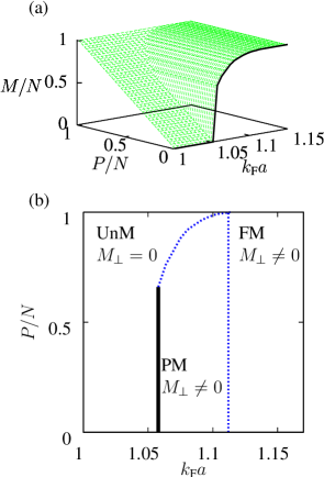
Figure 1: (a) shows the magnetization $M$ as a function of population imbalance, $P$ and interaction strength $k_{\text{F}}a=\sqrt[3]{3\pi^{2}(n_{\uparrow}+n_{\downarrow})}$ in the canonical ensemble at $T=0$ at fixed species populations. The thick line traces system variation at $P=0$ which corresponds to trap profile ($P/N=0$) in Fig. 3. (b) shows the phase boundary between “unmagnetized” (UnM) and partially magnetized (PM) region and the line of saturation before the fully-magnetized (FM) region. Note that, by unmagnetized, we refer to the not in-plane magnetization. The solid line denotes first order transitions, the dashed second order and saturation.

With the formal part of the analysis complete, we will now apply these results to explore the implications of ferromagnetism in the atomic Fermi gas. To begin, let us consider the phase behavior of the system in the canonical ensemble working at fixed particle number. The variation of the total magnetization, $|M|$, as a function of interaction strength and particle imbalance can be found by minimizing the free energy at fixed particle number. The results are shown in Fig. 1. To ensure that the free energy is locally minimized rather than just being at a stationary value Sheehy and Radzihovsky (2007b), the curvature was examined numerically. In the balanced Fermi gas, $P=0$, the results shown in Fig. 1(a) recapitulate those discussed by Duine and MacDonald (2005). In particular at zero temperature, when the interaction strength is small, $k_{\text{F}}a\lesssim 1.05$, there is no net magnetization. As the interaction strength is increased, at $k_{\text{F}}a\approx 1.05$ there is a first order phase transition into a magnetized phase with $M/N\approx 0.6$. As $k_{\text{F}}a$ is increased further the magnetization rises until it is saturated at $k_{\text{F}}a\approx 1.11$.

With increasing population imbalance, $P$, at $k_{\text{F}}a\lesssim 1.05$, where it is not energetically favorable for a spontaneous magnetization to develop, the magnetization is forced to stay pinned to the minimum value set by the imbalance. With increasing interaction strength, at $k_{\text{F}}a\approx 1.05$ there is a first order transition and the magnetization jumps to $M/N\approx 0.6$. This feature is consistent with the findings of the Stoner mean-field theory that the transition interaction strength found is independent of population imbalance. If the population imbalance is greater than $P/N\gtrsim 0.6$ then the magnetization takes the value of the spontaneous magnetization projected onto the sheet of minimum magnetization caused by the population imbalance.

From these results, one can infer the corresponding zero temperature phase diagram Fig. 1(b). Characterizing the phase behavior by the strength of the in-plane magnetization and the degree of polarization, the phase diagram divides into three distinct regions. At low interaction strength the system is not spontaneously unmagnetized, though there can be a magnetization fixed by the population imbalance. Then, at increased interaction strength the system become partially magnetized either through a first order (at low population imbalance) or a second order phase transition. At interaction strength above $k_{\text{F}}a\gtrsim 1.11$ the magnetization saturates.

To address the properties of the population imbalanced system in the grand canonical regime, we will divide our discussion between the uniform and trap geometries. In Sec. III.1 we will address the properties of a uniform system where the chemical potential $\mu$ and shift $\Delta\mu$ are held constant (allowing the species populations to effectively interchange). Drawing on these results, we will then discuss the phase behavior in a harmonic trap in Sec. III.2.

III.1 Uniform system

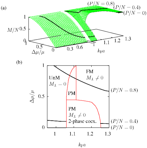
Figure 2: (Color online) (a) shows the variation of magnetization $M$ as a function of chemical potential shift $\Delta\mu$ and interaction strength $k_{\text{F}}a$ in the grand canonical ensemble at $T=0$. The thick lines correspond to trap profiles at $P/N=0$, $P/N=0.4$, and $P/N=0.8$ in Fig. 3. In the region where magnetization is undefined there is phase separation. The lower set of diagrams show the phase boundaries (and saturation line) between “unmagnetized” (UnM), partially magnetized (PM) and fully-magnetized (FM) regions, as well as the region of phase separation.

In the spatially uniform system, when the chemical potentials of the two species are fixed, for each value of the interaction strength $k_{\text{F}}a$ and relative shift in chemical potential $\Delta\mu/\mu$, from the free energy one can obtain the phase corresponding to minimal thermodynamic potential. Applying this procedure, the resulting phase behavior is shown in Fig. 2. For $\Delta\mu/\mu=0$ and small interaction strength $k_{\text{F}}a\lesssim 1.05$ there is no magnetization. As the interaction strength is increased, at $k_{\text{F}}a\approx 1.05$ in the canonical regime Fig. 1 there is a first order phase transition into a fully-magnetized state. Working at fixed chemical potential [Fig. 2(a)], the phase transition straight into a saturated state increases the number of particles, which in turn increases the effective interaction strength to $k_{\text{F}}a\approx 1.25$ (calculated using the chemical potential for a non-interacting system with the same total number of particles). This leads to an intermediate region of phase separation in the grand canonical regime. At $k_{\text{F}}a\lesssim 1.05$ as the chemical potential shift is increased up to $\Delta\mu/\mu=1$, the magnetization increases up to its maximum saturated value as the Fermi surfaces become more unbalanced. At $\Delta\mu/\mu>1$ the chemical potential of the minority spin species is negative so only the majority spin species remain and the system is fully magnetized. With a chemical potential shift the region of phase separation corresponds to the first order phase transition in Fig. 1. The corresponding phase diagram showing the regime of two-phase coexistence is shown in Fig. 2(b).

Finally, if the system has an imposed density and population imbalance, and the chemical potentials are free to vary, then there are two possibilities: Firstly, the spontaneous ferromagnetism is sufficient to provide the population imbalance and any excess magnetization lies in the plane. This corresponds to a point on the line $\Delta\mu=0$ in Fig. 2. The second possibility is that spontaneous ferromagnetism is not sufficient, and so there is an additional chemical potential shift $\Delta\mu\neq 0$. In this case the magnetization then points along the direction of population imbalance. This is consistent with the findings in Sec. II.4. For a given interaction strength, the magnetization increases with chemical potential shift to saturation, so there is always a chemical potential shift that will give a suitable population imbalance.

III.2 Trapped system

Using the insight gained from the study of the uniform system, we can now explore an atomic Fermi gas in the physical system — a potential trap. Without loss of generality we take $\uparrow$ ($\downarrow$) to represent the majority (minority) species of atoms. We focus on a harmonic trap, with rescaled spatial coordinates to ensure a spherically symmetric trapping potential, $V(\mathbf{r})\sim r^{2}$. Furthermore, we make use of the local density approximation in which the chemical potential of both species $\mu_{\text{eff},\sigma}(\mathbf{r})=\mu_{0,\sigma}-V(\mathbf{r})$ are renormalized by the same trapping potential. Although there is some experimental evidence Partridge et al. (2006a, b) that the local density approximation might not be valid De Silva and Mueller (2006); Imambekov et al. (2006) in some setups, we believe that its application here will correctly address the qualitative phase structure. The chemical potentials are regarded to be locally fixed, therefore the local phase is that of the uniform system in the grand canonical regime examined in Sec. III.1. With a constant chemical potential shift $\Delta\mu$ and interaction strength $g$, but varying effective chemical potential $\mu$, the system follows the trajectory $k_{\text{F}}a\propto\sqrt{\mu}$ and $\Delta\mu/\mu\propto 1/\mu$ in the grand canonical regime shown in Fig. 2. If the chemical potential is large, the system spontaneously becomes ferromagnetic, and the magnetization is saturated; if the chemical potential is small, the relative chemical potential shift is large ensuring the magnetization is again near saturation. The locus in Fig. 2 shows that, in the intermediate region, the magnetization can develop a minimum depending on the degree of population imbalance.

Figure 3: The density of particles at radius $r$ in a trap potential profile at three different values of total population imbalance. The variation in the local particle density $N$ is shown by the solid line, and the variation in the local magnetization $M$ is shown by the dashed line. The plot densities are renormalized by their central density, $N_{0}$, radii by the outer radius, $r_{0}$, of non-interacting particles with the same average inner chemical potential, $\mu_{0}$. The upper panel shows the effective $k_{\text{F}}a$ in the $P/N=0$ case.

To understand the behavior in the trap geometry, one should note the following: If the degree of equilibrium pseudo-spin magnetization is in excess of that imposed by total population imbalance alone, the analysis of Sec. II.4 tells us that some component of the spontaneous magnetization lies along the z-axis with the remainder oriented in the x-y plane. If, however, net population imbalance is large, then $\Delta\mu\neq 0$ and no in-plane magnetization develops. Here one may identify three characteristic behaviors with radial density profiles shown in Fig. 3. The first ($P/N=0$) has in-plane magnetization, and the others do not. The second ($P/N=0.4$) has a first order transition and non-zero phase separation whereas the third ($P/N=0.8$) is always fully magnetized due to strong interactions. The three plots all have the same central chemical potential.

The first possibility shown in Fig. 3($P/N=0$) is at small population imbalance, involving the development of a spontaneous magnetization which is in excess of what can be absorbed by population imbalance alone, in this case $\Delta\mu=0$ and some magnetization lies in the plane. At small radii, where the interaction strength $k_{\text{F}}a>1.25$ is greater than the limit for ferromagnetism, the results of the uniform system (Sec. III.1) show that there is saturated ferromagnetism in the plane and a normal component that provides the fixed population imbalance. Following this there is a region of phase separation and then at $k_{\text{F}}a\approx 1.05$ there are equal particle densities and no magnetization. The outer edge of the particle distribution of both species is where $\mu_{0}=V(r_{0})$.

In the second scenario shown in Fig. 3($P/N=0.4$) the spontaneous magnetization is not sufficient to provide population imbalance alone, in this case we require $\Delta\mu\neq 0$, and all magnetization is oriented along the axis of population imbalance. From the trap center the population imbalance is first fully saturated, followed by a region of phase separation, into a region of partial magnetization. This causes the minority spin particles to have a sharp maximum number density at $r/r_{0}\approx 0.6$, and the magnetization to have a corresponding minimum; this counters the intuitive expectation that number density should rise towards the trap center due to the increasing effective chemical potential. As the effective chemical potential continues to fall with increasing radius, the minority spin species population falls more rapidly than the majority and magnetization increases. At a large radius, the chemical potential of the minority spin particles reaches zero before the majority spin so there is a thin shell containing only majority spin particles at the outside and so is fully magnetized.

The third possibility shown in Fig. 3($P/N=0.8$) is that the locus in Fig. 2 does not cross the first order transition and region of phase separation. At $\Delta\mu/\mu<1$ the system is fully magnetized due to the strong interactions between particles. At $\Delta\mu/\mu>1$ the system is fully magnetized due to there being no minority spin particles. In the intermediate regime there is a narrow band where the system is partially polarized. The majority spin species exists out to greater radius than in cases ($P/N=0$) and ($P/N=0.4$) because $\Delta\mu$ is larger so a greater potential at a larger radius is required to give the majority spin species zero effective chemical potential.

IV Discussion

To conclude, let us now consider four methods of how spin magnetization could be detected experimentally. Firstly, the interaction energy can be estimated by studying the expansion of the gas Bourdel et al. (2003). Time of flight measurements of the expanding cloud with no external magnetic field $B=0$ are ballistic and so can provide the initial kinetic energy. If the magnetic field is present, $B\neq 0$, then interactions are significant during the expansion. Collisions ensure that all of the interaction energy is converted into kinetic energy so the measurements reflect the total released energy. Taking the difference between the $B\neq 0$ and $B=0$ measurements therefore probes the interaction energy. An unmagnetized gas has interaction energy whereas the fully magnetized gas has zero interaction energy so time of flight measurements should allow the ferromagnetic state to be detected.

Radio frequency spectroscopy Ketterle and Zwierlein (2008) allows one to probe the spatial variations of scattering lengths by exciting the atoms from one spin state $|1\rangle$ into some other state $|3\rangle$ whilst leaving the atoms in the second spin state $|2\rangle$ unaffected. The presence of atoms in state $|2\rangle$ shifts the resonance $\nu_{13}$ by $\Delta\nu_{13}=2n_{2}(a_{23}-a_{21})$, where $a_{ij}$ is the scattering length between states $|i\rangle$ and $|j\rangle$. Measurement of the resonance shift could allow the spatial distribution of the individual species to be probed. The presence of the ferromagnetic state could be inferred by looking for the characteristic density profiles outlined in Sec. III.1.

A third simple method of detecting a ferromagnetic transition could be to monitor the size of the atomic cloud. In a harmonic trap the cloud size is proportional to the square root of the Fermi energy. Therefore, the size of the fully-magnetized state is $2^{1/3}$ larger than the unmagnetized.

On the repulsive side of the Feshbach resonance three-body collisions can result in the formation of a molecular bound state of two atoms that might destroy the atomic gas before it has time to undergo ferromagnetic ordering. To overcome this obstacle an atomic gas spin could be polarized along the magnetic field direction and an RF $\pi/2$ pulse applied to rotate all the spins into the plane Ketterle and Zwierlein (2008). The rate of precession of the spins is set by the magnetic field strength, which varies across the atomic gas due to field inhomogeneities. The precession rate of the atoms would however be kept locked together by the ferromagnetic interaction. Furthermore the ferromagnetic phase has an antisymmetric wave function which inhibits collisions and so prevents the formation of molecular bound states. A signature of ferromagnetism is therefore the absence of molecular bound state formation.

We now outline two possible ways to further our analysis. The first order phase transition leads to discontinuities in the density and magnetization leading to phase separation. Such behavior could lead to a breakdown of the local density approximation, a potential source of inaccuracy in our analysis. This could be fixed through inclusion of a surface energy.

The second is to investigate the possibility that magnetic texture could develop. Textured modes may have been seen via the possible formation of a CDW/SDW in experimental results on the analogous solid state systems of itinerant electron ferromagnets $\text{UGe}_{2}$ Huxley et al. (2001); Watanabe and Miyake (2002), $\text{Ca}_{3}\text{Ru}_{2}\text{O}_{7}$ Baumberger et al. (2006), and MnSi Pfleiderer et al. (2001). Our general formalism should be able to be extended to include the possibility of a textured phase which lies beyond the first order line in the putative paramagnetic regime.

In conclusion we have developed a general formalism to describe itinerant ferromagnetic transitions in two-component fermionic cold atom systems with repulsive interactions, and potential population imbalance. At low population imbalance, we predict that the first order transition that characterizes the balanced system persists. However, when the imbalance is large the transition becomes continuous. In the trap geometry we found the first order phase transition led to discontinuities in density and magnetization. Up to a critical total population imbalance, set by the possible total magnetization following a first order transition, the phases in the trap had the same density and magnetization profiles with increasing population imbalance, but in-plane magnetization fell. With population imbalance above this level, the system requires a chemical potential shift to generate a population imbalance; however there is still a small range over which a first order phase transition is seen. In the two latter cases the local population imbalance displayed a characteristic minimum with radius.

Appendix A Computational analysis of momentum space integral

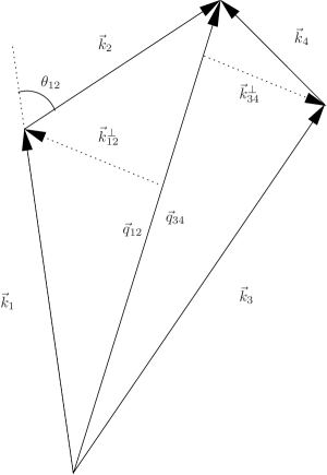
Figure 4: The re-parameterization of momenta used to ensure momentum conservation. $\mathbf{k}_{1,2,3,4}$ represent the momenta appearing in the original integral, whose separate sums are $\mathbf{q}_{12}=\mathbf{k}_{1}+\mathbf{k}_{2}$ and $\mathbf{q}_{34}=\mathbf{k}_{3}+\mathbf{k}_{4}$, which the Dirac delta function in Eq. (A) will ensure that $\mathbf{q}_{12}=\mathbf{q}_{34}$. $\theta_{12}$ represents the angle between $\mathbf{k}_{1}$ and $\mathbf{k}_{2}$, $\mathbf{k}_{12}^{\perp}$ is the vector perpendicular from $\mathbf{q}_{12}$ to $\mathbf{k}_{1}$ and $\mathbf{k}_{2}$, and $\mathbf{k}_{34}^{\perp}$ is similarly defined.

An important integral Eq. (II.3) encountered in this paper has the form

$$\iiiint F(|\mathbf{k}_{1}|,|\mathbf{k}_{2}|,|\mathbf{k}_{3}|,|\mathbf{k}_{4}|)\delta(\mathbf{k}_{1}+\mathbf{k}_{2}-\mathbf{k}_{3}-\mathbf{k}_{4})$$

$$\times d\mathbf{k}_{1}d\mathbf{k}_{2}d\mathbf{k}_{3}d\mathbf{k}_{4}\,.$$ (10)

To evaluate this integral one could substitute $\mathbf{k}_{4}=\mathbf{k}_{1}+\mathbf{k}_{2}-\mathbf{k}_{3}$, and then integrate over three parameters representing the lengths of vectors $\mathbf{k}_{1}$, $\mathbf{k}_{2}$, and $\mathbf{k}_{3}$, and a minimum of three relative angles between these vectors, giving a total of six integration parameters. However, numerical integration generally becomes more prohibitive with increasing number of dimensions. Since the function $F$ depends only on the magnitude of the momentum, the scheme outlined below allows us to perform the angular integration separately of the function and leave a numerical integral over just the four dimensions of the vector lengths.

The integral is re-parameterized according to Fig. 4, $\mathbf{q}_{12}=\mathbf{k}_{1}+\mathbf{k}_{2}$ and $\mathbf{q}_{34}=\mathbf{k}_{3}+\mathbf{k}_{4}$, the vector perpendicular from $\mathbf{q}_{12}$ to $\mathbf{k}_{1}$ and $\mathbf{k}_{2}$ is $\mathbf{k}_{12}^{\perp}$, and $\mathbf{k}_{34}^{\perp}$ is similarly defined. The vector $\mathbf{k}_{12}^{\perp}$ has length given by

$$k_{12}^{\perp}=\frac{1}{2q}\sqrt{2q^{2}\left(k_{1}^{2}+k_{2}^{2}\right)-q^{4}-\left(k_{1}^{2}-k_{2}^{2}\right)^{2}}\,.$$ (11)

We first concentrate on calculating the angular component just of the integral over $\mathbf{k}_{1}$ and $\mathbf{k}_{2}$, the angle between these vectors is $\theta_{12}$. The phase space volume of the angular integral is

$$\sin\theta_{12}d\theta_{12} \!\!=\!\!\!\! \frac{k_{12}^{\perp}}{k_{1}k_{2}}\left(\!2\!+\!\sqrt{\frac{k_{1}^{2}-k_{12}^{\perp 2}}{k_{2}^{2}-k_{12}^{\perp 2}}}+\sqrt{\frac{k_{2}^{2}-k_{12}^{\perp 2}}{k_{1}^{2}-k_{12}^{\perp 2}}}\right)dk_{12}^{\perp}$$ (12)

$$\!\!=\!\! -\frac{q_{12}}{k_{1}k_{2}}dq_{12}\,,$$

where $|k_{1}-k_{2}|\leq q_{12}\leq k_{1}+k_{2}$. The total number density integrated over two momenta can then be found using

$$\int_{0}^{\pi}4\pi k_{1}^{2}2\pi k_{2}^{2}\sin\theta_{12}d\theta_{12}$$

$$=\int_{|k_{1}-k_{2}|}^{k_{1}+k_{2}}4\pi k_{1}2\pi k_{2}q_{12}dq_{12}=4\pi k_{1}^{2}4\pi k_{2}^{2}\,,$$ (13)

which is the expected result. A similar procedure is used to parameterize the separate integral over the angular components of $\mathbf{k}_{3}$ and $\mathbf{k}_{4}$ into $\mathbf{q}_{34}$.

The original integral Eq. (A) is now re-written in terms of the parameters $q_{12}$ and $q_{34}$ using Eq. (A). Momentum conservation is required by the presence of the Dirac delta function $\delta(\mathbf{k}_{1}+\mathbf{k}_{2}-\mathbf{k}_{3}-\mathbf{k}_{4})=\delta(\mathbf{q}_{12}-\mathbf{q}_{34})$, however the $q_{12}$ and $q_{34}$ parameters introduced are just scalar quantities. The momentum conservation requirement is implemented by demanding that the two scalar integration parameters are equal, which sets the two integration parameters equal, $q_{12}=q_{34}=q$ so there is just one integral over parameter $q$ remaining. However, this introduces an extra angular degree of freedom (the angle between $\mathbf{q}_{12}$ and $\mathbf{q}_{34}$). In order to compensate the integrand is divided by the extra phase space volume of the angular integration, $4\pi q^{2}$. We then obtain

$$16\pi^{3}\iiiint F(k_{1},k_{2},k_{3},k_{4})k_{1}k_{2}k_{3}k_{4}$$

$$\times\max[0,\min(k_{1}+k_{2},k_{3}+k_{4})$$

$$-\max(|k_{1}-k_{2}|,|k_{3}-k_{4}|)]dk_{1}dk_{2}dk_{3}dk_{4}\,.$$ (14)

This integral is better suited to computational evaluation since it is four-dimensional [rather than the six-dimensional Eq. (A)], and the term introduced to compensate for the angular integral has a relatively simple form.

References

- Stwalley (1976) W. C. Stwalley, Phys. Rev. Lett. 37, 1628 (1976).
- Tiesinga et al. (1993) E. Tiesinga, B. J. Verhaar, and H. T. C. Stoof, Phys. Rev. A 47, 4114 (1993).
- Strecker et al. (2003) K. E. Strecker, G. B. Partridge, and R. G. Hulet, Phys. Rev. Lett. 91, 080406 (2003).
- Gupta et al. (2003) S. Gupta, M. W. Hadzibabic, Z. Zwierlein, C. A. Stan, . K. Dieckmann, C. H. Schunck, E. G. M. van Kempen, B. J. Verhaar, and W. Ketterle, Science 300, 1723 (2003).
- Chin et al. (2004) C. Chin, M. Bartenstein, A. Altmeyer, S. Riedl, S. Jochim, J. Hecker Denschlag, and R. Grimm, Science 305, 1128 (2004).
- Regal et al. (2004) C. A. Regal, M. Greiner, and D. S. Jin, Phys. Rev. Lett. 92, 040403 (2004).
- Stoner (1937) E. C. Stoner, Proc. R. Soc. London 165, 372 (1937).
- Wohlfarth and Rhodes (1962) E. P. Wohlfarth and P. Rhodes, Philos. Mag. 7, 1817 (1962).
- Ziman (1979) J. M. Ziman, Principles of the Theory of Solids (Cambridge University Press, 1979).
- Shimizu (1964) M. Shimizu, Proc. Phys. Soc. London 84, 397 (1964).
- Belitz et al. (1997) D. Belitz, T. R. Kirkpatrick, and T. Vojta, Phys. Rev. B 55, 9452 (1997).
- Belitz et al. (1999) D. Belitz, T. R. Kirkpatrick, and T. Vojta, Phys. Rev. Lett. 82, 4707 (1999).
- Vojta (2000) T. Vojta, Ann. Phys. 9, 403 (2000).
- Belitz and Kirkpatrick (2002) D. Belitz and T. R. Kirkpatrick, Phys. Rev. Lett. 89, 247202 (2002).
- Belitz et al. (2005) D. Belitz, T. R. Kirkpatrick, and J. Rollbühler, Phys. Rev. Lett. 94, 247205 (2005).
- Uhlarz et al. (2004) M. Uhlarz, C. Pfleiderer, and S. M. Hayden, Phys. Rev. Lett. 93, 256404 (2004).
- Uhlarz et al. (2005) M. Uhlarz, C. Pfleiderer, and S. M. Hayden, Physica B 359-361, 1174 (2005).
- Huxley et al. (2000) A. Huxley, I. Sheikin, and D. Braithwaite, Physica B 284-288, 1277 (2000).
- Pfleiderer et al. (2001) C. Pfleiderer, S. R. Julian, and G. G. Lonzarich, Nature (London) 414, 427 (2001).
- Yu et al. (2004) W. Yu, F. Zamborszky, J. D. Thompson, J. L. Sarrao, M. E. Torelli, Z. Fisk, and S. E. Brown, Phys. Rev. Lett. 92, 086403 (2004).
- Uemura et al. (2007) Y. Uemura, T. Goko, I. Gat-Malureanu, J. Carlo, P. Russo, A. Savici, A. Acze, G. MacDougall, J. Rodriguez, G. Luke, et al., Nature (London) 3, 29 (2007).
- Otero-Leal et al. (2009) M. Otero-Leal, F. Rivadulla, S. S. Saxena, K. Ahilan, and J. Rivas, Phys. Rev. B 79, 060401(R) (2009).
- Petrova et al. (2009) A. E. Petrova, V. N. Krasnorussky, T. A. Lograsso, and S. M. Stishov, Phys. Rev. B 79, 100401(R) (2009).
- Otero-Leal et al. (2008) M. Otero-Leal, F. Rivadulla, M. Garcia-Hernandez, A. Pineiro, V. Pardo, D. Baldomir, and J. Rivas, arXiv:cond-mat/0806.2819v1 [cond-mat.str-el] (2008).
- Misawa et al. (2008) T. Misawa, Y. Yamaji, and M. Imada, J. Phys. Jpn. 77, 093712 (2008).
- Hamlin et al. (2007) J. J. Hamlin, S. Deemyad, J. S. Schilling, M. K. Jacobsen, R. S. Kumar, A. L. Cornelius, G. Cao, and J. J. Neumeier, Phys. Rev. B 76, 014432 (2007).
- Liu and Hui (2006) X.-J. Liu and H. Hui, Europhys. Lett. 75, 364 (2006).
- Combescot (2007) R. Combescot, in Ultra-cold Fermi Gases, edited by M. Inguscio, W. Ketterle, and C. Salomon (IOS Press, 2007), vol. 164, p. 697.
- Sheehy and Radzihovsky (2007a) D. E. Sheehy and L. Radzihovsky, Ann. Phys. 322, 1790 (2007a).
- Sogo and Yabu (2002) T. Sogo and H. Yabu, Phys. Rev. A 66, 043611 (2002).
- Duine and MacDonald (2005) R. A. Duine and A. H. MacDonald, Phys. Rev. Lett. 95, 230403 (2005).
- Zhang et al. (2008) S. Zhang, H.-h. Hung, and C. Wu, arXiv:cond-mat/0805.3031v5 [cond-mat.str-el] (2008).
- Huxley et al. (2001) A. Huxley, I. Sheikin, E. Ressouche, N. Kernavanois, D. Braithwaite, R. Calemczuk, and J. Flouquet, Phys. Rev. B 63, 144519 (2001).
- Watanabe and Miyake (2002) S. Watanabe and K. Miyake, J. Phys. and Chem. Solids 63, 1465 (2002).
- Kitagawa et al. (2005) K. Kitagawa, K. Ishida, R. S. Perry, T. Tayama, T. Sakakibara, and Y. Maeno, Phys. Rev. Lett. 95, 127001 (2005).
- Berdnikov et al. (2008) I. Berdnikov, P. Coleman, and S. H. Simon, arXiv:0805.3693v1 [cond-mat.str-el] (2008).
- Keiter (1970) H. Keiter, Phys. Rev. B 2, 3777 (1970).
- Evenson et al. (1970) W. E. Evenson, J. R. Schrieffer, and S. Q. Wang, J. Appl. Phys. 41, 1199 (1970).
- Morandi et al. (1974) G. Morandi, E. Galleani d’Agliano, F. Napoli, and C. F. Ratto, Adv. Phys. 23, 867 (1974).
- Hubbard (1979) J. Hubbard, Phys. Rev. B 19, 2626 (1979).
- Prange and Korenman (1979a) R. E. Prange and V. Korenman, Phys. Rev. B 19, 4691 (1979a).
- Kanamori (1963) J. Kanamori, Prog. Theor. Phys. 30, 275 (1963).
- Hubbard (1963) J. Hubbard, Proc. R. Soc. London 276, 238 (1963).
- Abrikosov and Khalatnikov (1958) A. A. Abrikosov and I. M. Khalatnikov, Soviet Phys. JETP 6, 888 (1958).
- Prange and Korenman (1979b) R. E. Prange and V. Korenman, Phys. Rev. B 19, 4698 (1979b).
- Pathria (1996) R. K. Pathria, Statistical Mechanics (Butterworths, London, 1996).
- Sheehy and Radzihovsky (2007b) D. E. Sheehy and L. Radzihovsky, Phys. Rev. B 75, 136501 (2007b).
- Partridge et al. (2006a) G. B. Partridge, W. Li, R. I. Kamar, Y. Liao, and R. G. Hulet, Science 311, 503 (2006a).
- Partridge et al. (2006b) G. B. Partridge, W. Li, Y. A. Liao, R. G. Hulet, M. Haque, and H. T. C. Stoof, Phys. Rev. Lett. 97, 190407 (2006b).
- De Silva and Mueller (2006) T. N. De Silva and E. J. Mueller, Phys. Rev. A 73, 051602(R) (2006).
- Imambekov et al. (2006) A. Imambekov, C. J. Bolech, M. Lukin, and E. Demler, Phys. Rev. A 74, 053626 (2006).
- Bourdel et al. (2003) T. Bourdel, J. Cubizolles, L. Khaykovich, K. M. F. Magalhaes, S. J. J. M. F. Kokkelmans, G. V. Shlyapnikov, and C. Salomon, Phys. Rev. Lett. 91, 020402 (2003).
- Ketterle and Zwierlein (2008) W. Ketterle and M. W. Zwierlein, arXiv:cond-mat/0801.2500v1 [cond-mat.other] (2008).
- Baumberger et al. (2006) F. Baumberger, N. J. C. Ingle, N. Kikugawa, M. A. Hossain, W. Meevasana, R. S. Perry, K. M. Shen, D. H. Lu, A. Damascelli, A. Rost, et al., Phys. Rev. Lett. 96, 107601 (2006).