Aharonov-Bohm oscillations in disordered nanorings with quantum dots: Effect of electron-electron interactions

Abstract

We investigate the effect of electron-electron interactions on Aharonov-Bohm (AB) current oscillations in nanorings formed by a chain of metallic quantum dots. We demonstrate that electron-electron interactions cause electron dephasing thereby suppressing the amplitude of AB oscillations at all temperatures down to $T=0$. The crossover between thermal and quantum dephasing is found to be controlled by the ring perimeter. Our predictions can be directly tested in future experiments.

,

1 Introduction

Coherent electrons propagating along different paths in multiply connected conductors, such as, e.g., metallic rings, can interfere causing a specific quantum contribution to the system conductance $\delta G$. Threading the ring by an external magnetic flux $\Phi$ one can control the relative phase of the wave functions of interfering electrons, thus changing the magnitude of $\delta G$ as a function of $\Phi$. The dependence $\delta G(\Phi)$ turns out to be periodic with the fundamental period equal to the flux quantum $\Phi_{0}=hc/e$. These Aharonov-Bohm (AB) conductance oscillations represent one of the fundamental low temperature properties of meso- and nanoscale conductors [1].

In diffusive conductors electrons can propagate along numerous different paths picking up different phases. Averaging over such random phases usually washes out AB oscillations $\delta G(\Phi)$ with the period $\Phi_{0}$ in the presence of disorder [1]. There exists, however, a special class of electron trajectories which interference is not sensitive to averaging over disorder. These are pairs of time-reversed paths which are also responsible for the phenomenon of weak localization [2]. In disordered rings interference between these trajectories gives rise to non-vanishing AB oscillations with the principal period $\Phi_{0}/2$. Such oscillations will be analyzed below in this paper.

It is well established that interactions between electrons and other degrees of freedom can lead to their decoherence thus reducing electron’s ability to interfere. Hence, AB oscillations can be used as a tool to probe the fundamental effect of interactions on quantum coherence of electrons in nanoscale conductors. Recently it was demonstrated [3, 4, 5] that the effect of quantum decoherence by electron-electron interactions can be conveniently studied employing the model of a system of coupled quantum dots. This model embraces practically all types of disordered conductors and allows for a straightforward non-perturbative treatment of electron-electron interactions. Very recently we employed a similar model in order to study the effect of electron-electron interactions on AB oscillations in nanorings with two quantum dots [6]. In this paper we further extend the approach [6] to nanorings containing arbitrary number of quantum dots $N$. In the limit of large $N$ this system serves as a model for diffusive nanorings.

The structure of our paper is as follows. In Sec. 2 we will address nanorings with two quantum dots [6]. For this simpler example we will specify our general real time path integral formalism and recapitulate our main results [6]. In Sec. 3 we will generalize our analysis adopting it to nanorings consisting of many quantum dots. The paper is concluded by a brief discussion in Sec. 4.

2 Nanorings with two quantum dots

2.1 The model and basic formalism

In this section we will consider the system depicted in Fig. 1. The structure consists of two chaotic quantum dots (L and R) characterized by mean level spacing $\delta_{L}$ and $\delta_{R}$ which are the lowest energy parameters in our problem. These (metallic) dots are interconnected via two tunnel junctions J₁ and J₂ with conductances $G_{t1}$ and $G_{t2}$ forming a ring-shaped configuration as shown in Fig. 1. The left and right dots are also connected to the leads (LL and RL) respectively via the barriers J_L and J_R with conductances $G_{L}$ and $G_{R}$. We also define the corresponding dimensionless conductances of all four barriers as $g_{t1,2}=G_{t1,2}R_{q}$ and $g_{L,R}=G_{t1,2}R_{q}$, where $R_{q}=2\pi/e^{2}$ is the quantum resistance unit.

Following [6] we will assume that dimensionless conductances $g_{L,R}$ are much larger than unity, while the conductances $g_{t1}$ and $g_{t2}$ are small as compared to those of the outer barriers, i.e.

$$g_{L},g_{R}\gg 1,g_{t1},g_{t2}.$$ (1)

The whole structure is pierced by the magnetic flux $\Phi$ through the hole between two central barriers in such way that electrons passing from left to right through different junctions acquire different geometric phases. Applying a voltage across the system one induces the current which shows AB oscillations with changing the external flux $\Phi$.

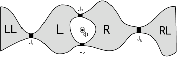
Figure 1: The ring-shaped quantum dot structure under consideration.

The system depicted in Fig. 1 is described by the effective Hamiltonian:

$$\hat{H} = \sum_{i,j=L,R}\frac{C_{ij}\hat{\bm{V}}_{i}\hat{\bm{V}}_{j}}{2}+\hat{\bm{H}}_{LL}+\hat{\bm{H}}_{RL}$$ (2)

$$+\sum_{j=L,R}\hat{\bm{H}}_{j}+\hat{\bm{T}}_{L}+\hat{\bm{T}}_{R}+\hat{\bm{T}},$$

where $C_{ij}$ is the capacitance matrix, $\hat{\bm{V}}_{L(R)}$ is the electric potential operator on the left (right) quantum dot,

$$\hat{\bm{H}}_{LL}=\sum\limits_{\alpha=\uparrow,\downarrow}\int\limits_{LL}d^{3}{\bm{r}}\hat{\Psi}^{\dagger}_{\alpha,LL}({\bm{r}})(\hat{H}_{LL}-eV_{LL})\hat{\Psi}_{\alpha,LL}({\bm{r}}),$$

$$\hat{\bm{H}}_{RL}=\sum\limits_{\alpha=\uparrow,\downarrow}\int\limits_{RL}d^{3}{\bm{r}}\hat{\Psi}^{\dagger}_{\alpha,RL}({\bm{r}})(\hat{H}_{RL}-eV_{RL})\hat{\Psi}_{\alpha,RL}({\bm{r}})$$

are the Hamiltonians of the left and right leads, $V_{LL,RL}$ are the electric potentials of the leads fixed by the external voltage source,

$$\hat{\bm{H}}_{j}=\sum\limits_{\alpha=\uparrow,\downarrow}\int\limits_{j}d^{3}{\bm{r}}\hat{\Psi}^{\dagger}_{\alpha,j}({\bm{r}})(\hat{H}_{j}-e\hat{\bm{V}}_{j})\hat{\Psi}_{\alpha,j}({\bm{r}})$$

defines the Hamiltonians of the left ($j=L$) and right ($j=R$) quantum dots and

$$\hat{H}_{j}=\frac{(\hat{p}_{\mu}-\frac{e}{c}A_{\mu}(r))^{2}}{2m}-\mu+U_{j}(r)$$

is the one-particle Hamiltonian of electron in $j$-th quantum dot with disorder potential $U_{j}(r)$. Electron transfer between the left and the right quantum dots will be described by the Hamiltonian

$$\hat{\bm{T}}=\sum_{\alpha=\uparrow,\downarrow}\int_{J_{1}+J_{2}}d^{2}{\bm{r}}\,\big{[}t({\bm{r}})\hat{\Psi}^{\dagger}_{\alpha,L}({\bm{r}})\hat{\Psi}_{\alpha,R}({\bm{r}})+{\rm c.c.}\big{]}.$$

The Hamiltonian $\hat{\bm{T}}_{L(R)}$ describing electron transfer between the left dot and the left lead (the right dot and the right lead) is defined analogously.

Following [6] we will describe the time evolution of the density matrix of our system by means of the standard equation

$$\hat{\rho}(t)=e^{-i\hat{H}t}\hat{\rho}_{0}\,e^{i\hat{H}t},$$ (3)

where $\hat{H}$ is given by Eq. (2). Let us express the operators $e^{-i\hat{H}t}$ and $e^{i\hat{H}t}$ via path integrals over the fluctuating electric potentials $V_{j}^{F,B}$ defined respectively on the forward and backward parts of the Keldysh contour:

$$e^{-i\hat{H}t} = \int DV_{j}^{F}\;{\rm T}\,\exp\left\{-i\int_{0}^{t}dt^{\prime}\hat{H}\left[V_{j}^{F}(t^{\prime})\right]\right\},$$

$$e^{i\hat{H}t} = \int DV_{j}^{B}\;\tilde{\rm T}\,\exp\left\{i\int_{0}^{t}dt^{\prime}\hat{H}\left[V_{j}^{B}(t^{\prime})\right]\right\}.$$ (4)

Here ${\rm T}\,\exp$ ($\tilde{\rm T}\,\exp$) stands for the time ordered (anti-ordered) exponent.

Let us define the effective action of our system

$$iS[V^{F},V^{B}] = \ln\left({\rm tr}\left[{\rm T}\,\exp\left\{-i\int_{0}^{t}dt^{\prime}\hat{H}\left[V_{j}^{F}(t^{\prime})\right]\right\}\right.\right.$$ (5)

$$\times\,\left.\left.\hat{\rho}_{0}\tilde{\rm T}\,\exp\left\{i\int_{0}^{t}dt^{\prime}\hat{H}\left[V_{j}^{B}(t^{\prime})\right]\right\}\right]\right)$$

Integrating out the fermionic variables we rewrite the action in the form

$$iS=iS_{C}+iS_{ext}+2\bf Tr\ln\left[\check{G}^{-1}\right].$$ (6)

Here $S_{C}$ is the standard term describing charging effects, $S_{ext}$ accounts for an external circuit and

$${\bf\check{G}^{-1}}=\left(\begin{array}[]{cccc}\hat{G}^{-1}_{LL}&\hat{T}_{L}&0&0\\ \hat{T}^{\dagger}_{L}&\hat{G}^{-1}_{L}&\hat{T}&0\\ 0&\hat{T}^{\dagger}&\hat{G}^{-1}_{R}&\hat{T}_{R}\\ 0&0&\hat{T}^{\dagger}_{R}&\hat{G}^{-1}_{RL}\end{array}\right).$$ (7)

is the inverse Green-Keldysh function of electrons propagating in the fluctuating fields. Here each quantum dot as well as two leads is represented by the 2x2 matrix in the Keldysh space:

$$\hat{G}^{-1}_{i}=\left(\begin{array}[]{cc}i\partial_{t}-\hat{H}_{i}+eV^{F}_{i}&0\\ 0&-i\partial_{t}+\hat{H}_{i}-eV^{B}_{i}\end{array}\right)$$ (8)

2.2 Effective action

Let us expand the exact action $iS$ (6) in powers of $\hat{T}$. Keeping the terms up to the fourth order in the tunneling amplitude, we obtain

$$iS\approx iS_{C}+iS_{ext}+iS_{L}+iS_{R}-2{\bf tr}\left[\hat{G}_{L}\hat{T}\hat{G}_{R}\hat{T}^{\dagger}\right]$$

$$-{\bf tr}\left[\hat{G}_{L}\hat{T}\hat{G}_{R}\hat{T}^{\dagger}\hat{G}_{L}\hat{T}\hat{G}_{R}\hat{T}^{\dagger}\right].$$ (9)

Here $iS_{L,R}$ are the contributions of isolated dots, the terms $\propto t^{2}$ yield the Ambegaokar-Eckern-Schön (AES) action [7] $iS^{AES}$ described by the diagram in Fig. 2a, and the fourth order terms $\propto t^{4}$ account for the weak localization correction to the system conductance [4, 5].

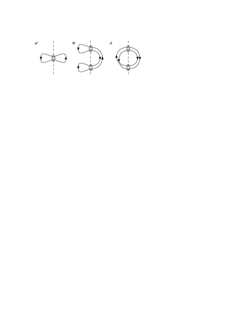
Figure 2: Diagrammatic representation of different contributions originating from expansion of the effective action in powers of the central barrier transmissions: second order (AES) terms (a) and different fourth order terms (b,c).

It is easy to demonstrate [6] that after disorder averaging $iS^{AES}$ becomes independent of $\Phi$ and, hence, it does not account for the AB effect investigated here. Averaging the last term in Eq. (9) over realizations of transmission amplitudes and over disorder one can show [6] that only the contribution generated by the diagram (c) depends on the magnetic flux. It yields [6]

$$iS^{WL}_{\Phi}=-\frac{ig_{t1}g_{t2}}{4\pi^{2}N_{L}N_{R}}\sum\limits_{m,n=1,2}e^{2i(\varphi_{g}^{(n)}-\varphi_{g}^{(m)})}$$

$$\times\int d\tau_{1}d\tau_{2}\int dt_{1}...dt_{4}C_{L}(\tau_{1})C_{R}(\tau_{2})\qquad\qquad$$

$$\times e^{i(\varphi^{+}(t_{2})-\varphi^{+}(t_{3})+\varphi^{+}(t_{4})-\varphi^{+}(t_{1}))}\sin\frac{\varphi^{-}(t_{1})}{2}$$

$$\times\left[h(t_{1}-t_{2}-\tau_{1})e^{i\frac{\varphi^{-}(t_{2})}{2}}+\right.\qquad\qquad\qquad\qquad$$

$$\left.+f(t_{1}-t_{2}-\tau_{1})e^{-i\frac{\varphi^{-}(t_{2})}{2}}\right]$$

$$\times\left[h(t_{2}-t_{3}-\tau_{2})e^{-i\frac{\varphi^{-}(t_{3})}{2}}f(t_{3}-t_{4}+\tau_{1})-\right.\quad$$

$$\left.-f(t_{2}-t_{3}-\tau_{2})e^{i\frac{\varphi^{-}(t_{3})}{2}}h(t_{3}-t_{4}+\tau_{1})\right]$$

$$\times\left[e^{i\frac{\varphi^{-}(t_{4})}{2}}f(t_{4}-t_{1}+\tau_{2})+\right.\qquad\qquad\qquad\qquad$$

$$\left.+e^{-i\frac{\varphi^{-}(t_{4})}{2}}h(t_{4}-t_{1}+\tau_{2})\right]$$

$$+\{L\leftrightarrow R,\varphi^{\pm}\rightarrow-\varphi^{\pm}\},$$ (10)

where $C_{L,R}(t)$ the Cooperons in the left and right dots, $f(t)=\int f(E)dE/2\pi$ is the Fourier transform of the Fermi function $f(E)=(\exp(E/T)+1)^{-1}$ and $h(t)=\delta(t)-f(t)$. Here we also introduced the geometric phases $\varphi_{g}^{(1,2)}=\frac{e}{c}\int\limits_{L}^{R}dx_{\mu}A_{\mu}(x)$, where the integration contour starts in the left dot, crosses the first ($\varphi_{g}^{(1)}$) or the second ($\varphi_{g}^{(2)}$) junction and ends in the right dot. The difference between these two geometric phases is $\varphi_{g}^{(1)}-\varphi_{g}^{(2)}=2\pi\Phi/\Phi_{0}$. In addition, we defined the “classical” and the “quantum” components of the fluctuating phase: $\varphi^{+}(t)=(\varphi_{F}(t)+\varphi_{B}(t))/2$, $\varphi^{-}(t)=\varphi_{F}(t)-\varphi_{B}(t)$ where the phases $\varphi_{F,B}(t)=e\int^{t}d\tau(V^{F,B}_{R}(\tau)-V^{F,B}_{L}(\tau))$ are defined on the forward and backward parts of the Keldysh contour.

The above expression for the action $S^{WL}_{\Phi}$ (10) fully accounts for coherent oscillations of the system conductance in the lowest non-vanishing order in tunneling.

2.3 Aharonov-Bohm conductance

Let us now evaluate the current $I$ through our system. This current can be split into two parts, $I=I_{0}+\delta I$, where $I_{0}$ is the flux-independent contribution and $\delta I$ is the quantum correction to the current sensitive to the magnetic flux $\Phi$. This correction is determined by the action $iS^{WL}_{\Phi}$, i.e.

$$\delta I=-e\int\mathcal{D}^{2}\varphi^{\pm}\frac{\delta S^{WL}_{\Phi}[\varphi^{+},\varphi^{-}]}{\delta\varphi^{-}(t)}e^{iS[\varphi^{+},\varphi^{-}]}.$$ (11)

Below we will only be interested in finding the quantum correction (11).

In order to evaluate the path integral over the phases $\varphi^{\pm}$ in (11) we note that in the interesting for us metallic limit (1) phase fluctuations can be considered small down to exponentially low energies [8, 9] in which case it suffices to expand both contributions up to the second order $\varphi^{\pm}$. Moreover, this Gaussian approximation becomes exact [10, 11, 12] in the limit of fully open left and right barriers with $g_{L,R}\gg 1$. Thus, in the metallic limit (1) the integral (11) remains Gaussian at all relevant energies and can easily be performed.

This task can be accomplished with the aid of the following correlation functions

$$\langle\varphi^{+}(t)\rangle=eVt,\qquad\langle\varphi^{-}(t)\rangle=0,$$ (12)

$$\langle(\varphi^{+}(t)-\varphi^{+}(0))\varphi^{+}(0)\rangle=-F(t),$$ (13)

$$\langle\varphi^{+}(t)\varphi^{-}(0)+\varphi^{-}(t)\varphi^{+}(0)\rangle=2iK(|t|),$$ (14)

$$\langle\varphi^{+}(t)\varphi^{-}(0)-\varphi^{-}(t)\varphi^{+}(0)\rangle=2iK(t),$$ (15)

$$\langle\varphi^{-}(t)\varphi^{-}(0)\rangle=0,$$ (16)

where the last relation follows directly from the causality principle [13]. Here and below we define $V=V_{RL}-V_{LL}$ to be the transport voltage across our system.

Note that the above correlation functions are well familiar from the so-called $P(E)$-theory[7, 15] describing electron tunneling in the presence of an external environment which can also mimic electron-electron interactions in metallic conductors. They are expressed in terms of an effective impedance $Z(\omega)$ “seen” by the central barriers J₁ and J₂

$$F(t)=e^{2}\int\frac{d\omega}{2\pi}\coth\frac{\omega}{2T}\Re[Z(\omega)]\frac{1-\cos(\omega t)}{\omega},$$ (17)

$$K(t)=e^{2}\int\frac{d\omega}{2\pi}\Re[Z(\omega)]\frac{\sin(\omega t)}{\omega}.$$ (18)

Further evaluation of these correlation functions for our system is straightforward and yields

$$F(t)\simeq\frac{4}{g}\left(\ln\left|\frac{\sinh(\pi Tt)}{\pi T\tau_{RC}}\right|+\gamma\right),$$ (19)

$$K(t)\simeq\frac{2\pi}{g}{\rm sign}(t),$$ (20)

where we defined $g=4\pi/e^{2}Z(0)$ and $\gamma\simeq 0.577$ is the Euler constant. Neglecting the contribution of external leads and making use of the inequality (1) we obtain $g\simeq 2g_{L}g_{R}/(g_{L}+g_{R})$. We observe that while $F(t)$ grows with time at any temperature including $T=0$, the function $K(t)$ always remains small and it can be safely ignored in the leading order in $1/g\ll 1$. After that the Fermi function $f(E)$ drops out from the final expression for the quantum correction to the current [4, 5, 6]. Hence, the amplitude of AB oscillations is affected by the electron-electron interaction only via the correlation functions for the “classical” component of the Hubbard-Stratonovich phase $\varphi^{+}$.

The expression for the current takes the form

$$\delta I(\Phi)=-I_{AB}\cos(4\pi\Phi/\Phi_{0})-I_{WL1}-I_{WL2},$$ (21)

where the first – flux dependent – term in the right-hand side explicitly accounts for AB oscillations, while the terms $I_{WL1,2}$ represent the remaining part of the quantum correction to the current [4] which does not depend on $\Phi$.

Let us restrict our attention to the case of two identical quantum dots with volume $\mathcal{V}$, dwell time $\tau_{D}$ and dimensionless conductances $g_{L}=g_{R}\equiv g=4\pi/\delta\tau_{D}$, where $\delta=1/\mathcal{V}\nu$ is the dot mean level spacing and $\nu$ is the electron density of states. In this case the Cooperons take the form $C_{L}(t;{\bf x},{\bf y})=C_{R}(t;{\bf x},{\bf y})=(\theta(t)/\mathcal{V})e^{-t/\tau_{D}}$. We obtain [6]

$$I_{AB}=\frac{e^{2}g_{t1}g_{t2}\delta^{2}V}{4\pi^{3}}\int\limits_{0}^{\infty}d\tau_{1}d\tau_{2}e^{-\frac{\tau_{1}+\tau_{2}}{\tau_{D}}-\mathcal{F}(\tau_{1},\tau_{2})}.$$ (22)

where $\mathcal{F}=2F(\tau_{1})+2F(\tau_{2})-F(\tau_{1}-\tau_{2})-F(\tau_{1}+\tau_{2})$.

In the absence of electron-electron interactions this formula yields $I_{AB}^{(0)}=4e^{2}g_{t1}g_{t2}V/(\pi g^{2})$. In order to account for the effect of interactions we substitute Eq. (19) into Eq. (22). Performing time integrations at high enough temperatures we obtain

$$\frac{I_{AB}}{I_{AB}^{(0)}}=\left\{\begin{array}[]{lc}e^{-\frac{8\gamma}{g}}\frac{(2\pi T\tau_{RC})^{8/g}}{1+4\pi T\tau_{D}/g},&\tau_{D}^{-1}\lesssim T\lesssim\tau_{RC}^{-1},\\ \frac{1}{2\tau_{D}}\left(\frac{g\tau_{RC}}{T}\right)^{1/2},&\tau_{RC}^{-1}\lesssim T,\end{array}\right.$$ (23)

while in the low temperature limit we find

$$\frac{I_{AB}}{I_{AB}^{(0)}}=e^{-\frac{8\gamma}{g}}\left(\frac{2\tau_{RC}}{\tau_{D}}\right)^{8/g},\qquad T\lesssim\tau_{D}^{-1}.$$ (24)

The above results demonstrate that interaction-induced suppression of AB oscillations in metallic dots with $\tau_{RC}\ll\tau_{D}$ persists down to $T=0$. The fundamental reason for this suppression is that the interaction of an electron with an effective environment (produced by other electrons) effectively breaks down the time-reversal symmetry and, hence, causes both dissipation and dephasing for interacting electrons down to $T=0$ [13]. In this respect it is also important to point out a deep relation between interaction-induced electron decoherence and the $P(E)$-theory [7, 15] which we already emphasized elsewhere [4, 5].

3 Ring composed of a chain of quantum dots

Let us now turn to the central part of the present work, i.e. to the analysis of AB oscillations in nanorings composed of a chain of quantum dots, as shown in Fig. 3. In the previous section we already demonstrated that the dominant effect of electron-electron interactions is electron dephasing fully determined by fluctuations of the phase $\varphi^{+}$. At the same time fluctuations of the phase $\varphi^{-}$ turn out to be essentially irrelevant for the whole issue. This conclusion is general being independent of the number of quantum dots in the ring. Hence, in order address the problem in the many-dot configuration of Fig. 3 it suffices to ignore the fluctuating field $\varphi^{-}$ and account only for the phase $\varphi^{+}$. This observation yields significant simplifications in our calculation to be presented below.

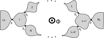
Figure 3: Ring composed of $N$ quantum dots

For simplicity we will consider the case of identical quantum dots (with mean level spacing $\delta$ and dwell time $\tau_{D}=2\pi/(g\delta)$) coupled by junctions with conductances $g_{t}$ and the Fano-factor $\beta_{t}$. Leads are coupled to the ring at the dots with numbers $1$ and $L+1$ by junctions with conductance $g$. Interference correction to the conductance of n-th junction was derived by means of the non-linear sigma-model approach [3] which yields

$$\delta G_{1}=-\frac{e^{2}g_{t}\delta}{4\pi^{2}}\int\limits_{0}^{\infty}dt[\beta_{t}C_{n,n+1}(t)e^{\frac{4\pi i\Phi}{N\Phi_{0}}}+$$

$$+(1-\beta_{t})(C_{n,n}(t)+C_{n+1,n+1}(t))+$$

$$+\beta_{t}C_{n+1,n}(t)e^{-\frac{4\pi i\Phi}{N\Phi_{0}}}],$$ (25)

where $C_{m,n}(t)$ is the Cooperon. The quantum correction to conductance of the whole system can be obtained with the aid of the Kirchhoff’s law. For the case $Ng\ll g_{t}$ considered here one finds

$$\delta G=\frac{NL(N-L)g^{2}}{(2Ng_{t}+L(N-L)g)^{2}}\delta g\approx\frac{L(N-L)g^{2}}{4Ng_{t}^{2}}\delta G_{1}.$$ (26)

In the absence of electron-electron interactions $C_{m,n}(t)$ satisfies the diffusion-like equation which reads

$$\frac{\partial C_{n,m}(t)}{\partial t}+\frac{2C_{n,m}(t)-C_{n+1,m}(t)e^{-\frac{4\pi i\Phi}{N\Phi_{0}}}}{2\tau_{D}}-$$

$$-\frac{C_{n-1,m}(t)e^{\frac{4\pi i\Phi}{N\Phi_{0}}}}{2\tau_{D}}=\delta_{n,m}\delta(t)$$ (27)

in the case $n\neq 1,L+1$ and

$$\frac{\partial C_{n,m}(t)}{\partial t}+\frac{2C_{n,m}(t)-C_{n+1,m}(t)e^{-\frac{4\pi i\Phi}{N\Phi_{0}}}}{2\tau_{D}}-$$

$$-\frac{C_{n-1,m}(t)e^{\frac{4\pi i\Phi}{N\Phi_{0}}}}{2\tau_{D}}+\frac{g\delta}{4\pi}C_{n,m}(t)=\delta_{n,m}\delta(t)$$ (28)

for $n=1$ or $n=L+1$. The solution of the above diffusion equation can be represented in the form of the “functional integral”, which has the following form:

$$C_{n,m}^{(0)}(t)=\sum\limits_{k=|n-m|}^{\infty}\sum\limits_{\nu(0)=n}^{\nu(t)=m}e^{\frac{4\pi i(n-m+NW[\nu(t)])\Phi}{N\Phi_{0}}}\times$$

$$\times\int\limits_{0}^{t}dt_{k}\int\limits_{0}^{t_{k}}dt_{k-1}...\int\limits_{0}^{t_{2}}dt_{1}\frac{e^{-\frac{t}{\tau_{D}}}}{(2\tau_{D})^{k}}.$$ (29)

Here the summation is performed over all discrete trajectories with fixed endpoints and $W[\nu(t)]$ denotes the winding number for a given trajectory.

Let us now include electron-electron interactions. Taking into account only the $V^{+}$-component of the fluctuating field one can easily incorporate the effect of interactions into the above expression for the Cooperon. One finds

$$C_{n,m}(t)=\sum\limits_{k=|n-m|}^{\infty}\sum\limits_{\nu(0)=n}^{\nu(t)=m}e^{\frac{4\pi i(n-m+NW[\nu(t)])\Phi}{N\Phi_{0}}}\times$$

$$\times\int\limits_{0}^{t}dt_{k}...\int\limits_{0}^{t_{2}}dt_{1}\frac{e^{-\frac{t}{\tau_{D}}+ie\int\limits_{0}^{t}d\tau(V^{+}_{\nu(\tau)}(\tau)-V^{+}_{\nu(\tau)}(t-\tau))}}{(2\tau_{D})^{k}},$$ (30)

i.e. the fluctuating field $V^{+}$ just modifies the phases of the electron wave functions. Averaging over Gaussian fluctuations of $V^{+}$ we get

$$\Bigl{\langle}\exp\Bigl{[}ie\int\limits_{0}^{t}d\tau(V_{\nu(\tau)}(\tau)-V_{\nu(\tau)}(t-\tau))\Bigl{]}\Bigr{\rangle}_{V^{+}}=$$

$$=\exp\Bigl{[}-e^{2}\int\limits_{0}^{t}d\tau_{1}d\tau_{2}(F_{\nu(\tau_{1}),\nu(\tau_{2})}(\tau_{1}-\tau_{2})-$$

$$-F_{\nu(\tau_{1}),\nu(\tau_{2})}(t-\tau_{1}-\tau_{2}))\Bigr{]}.$$ (31)

Here $F_{m,n}(t)=\langle V^{+}_{m}(t)V^{+}_{n}(0)\rangle_{V^{+}}$ defines the correlator for fluctuating voltages.

In order to evaluate the Cooperon in the presence of interactions let us first expand the exponent in Eq. (31) in Taylor series, then perform the summation over all trajectories and after that re-exponentiate the result. This procedure is equivalent to the substitution $\langle\langle e^{F}\rangle\rangle\rightarrow e^{\langle\langle F\rangle\rangle}$ which – although not exact – is known to provide sufficiently accurate results for the problem in question at all time scales (cf., e.g., Ref. [16]).

Averaging over diffusive pathes is performed with the aid of the diffuson $D_{m,n}(t)$:

$$\langle\langle F_{\nu(\tau_{1}),\nu(\tau_{2})}(\tau_{1}-\tau_{2})\rangle\rangle=\qquad\qquad\qquad\qquad$$

$$=\frac{1}{N}\sum\limits_{m,n=1}^{N}F_{m,n}(\tau_{1}-\tau_{2})D_{m,n}(|\tau_{1}-\tau_{2}|)$$ (32)

As a result one finds [5]

$$C_{m,n}(t)=C_{m,n}^{(0)}(t)e^{-\mathcal{F}(t)},$$ (33)

where

$$\mathcal{F}(t)=\frac{e^{2}}{N}\sum\limits_{n,m=1}^{N}\int\limits_{0}^{t}d\tau_{1}d\tau_{2}F_{m,n}(\tau_{1}-\tau_{2})\times$$

$$\times\left(D_{m,n}(|\tau_{1}-\tau_{2}|)-D_{m,n}(|t-\tau_{1}-\tau_{2}|)\right).$$ (34)

The correlator for fluctuating voltages can be derived, e. g., by means of the non-linear sigma model [3] which yields

$$F_{m,n}(t)=\frac{\tau_{D}}{N}\sum\limits_{q=1}^{N}\int\frac{d\omega}{2\pi}e^{-i\omega t}\omega\coth\frac{\omega}{2T}\frac{f(q)e^{\frac{2\pi iq}{N}(m-n)}}{\omega^{2}\tau_{D}^{2}+\varepsilon^{2}(q)}$$ (35)

where

$$f(q)=\frac{g_{t}\tau_{D}e^{2}}{\pi}\frac{\epsilon(q)}{(4C\epsilon(q)+C_{g})^{2}},$$ (36)

$$\varepsilon(q)=\epsilon(q)+\frac{g_{t}\tau_{D}e^{2}}{\pi}\frac{\epsilon(q)}{4C\epsilon(q)+C_{g}}$$ (37)

and $\epsilon(q)=1-\cos\frac{2\pi q}{N}$. As above, here $C$ and $C_{g}$ denote respectively the junction and the dot capacitances.

Finally we specify the expressions for the diffuson and the Cooperon in the absence of electron-electron interactions. They read

$$D_{m,n}(t)=\frac{\tau_{D}}{N}\sum\limits_{q=1}^{N}\int\frac{d\omega}{2\pi}\frac{e^{-i\omega t+\frac{2\pi iq}{N}(m-n)}}{-i\omega\tau_{D}+\epsilon(q)}.$$ (38)

$$C_{m,n}^{(0)}(t)=\frac{\tau_{D}}{N}\sum\limits_{q=1}^{N}\int\frac{d\omega}{2\pi}\frac{e^{-i\omega t+\frac{2\pi iq}{N}(m-n)}}{-i\omega\tau_{D}+\epsilon(q-2\Phi/\Phi_{0})}.$$ (39)

The above equations are sufficient to evaluate the function $\mathcal{F}(t)$ in a general form. Here we are primarily interested in AB oscillations and, hence, we only need to account for the flux-dependent contributions determined by the electron trajectories which fully encircle the ring at least once. Obviously, one such traverse around the ring takes time $t\geq N^{2}\tau_{D}$. Hence, the behavior of the function $\mathcal{F}(t)$ only at such time scales needs to be studied for our present purposes. In this long time limit $\mathcal{F}(t)$ is a linear function of time with the corresponding slope

$$\mathcal{F}^{\prime}(t\geq N^{2}\tau_{D})\approx\qquad\qquad\qquad\qquad\qquad\qquad\qquad$$

$$\approx\frac{2e^{2}\tau_{D}^{2}}{N}\sum\limits_{q=1}^{N-1}\int\frac{d\omega}{2\pi}\frac{f(q)\epsilon(q)\omega\coth\frac{\omega}{2T}}{(\omega^{2}\tau_{D}^{2}+\epsilon^{2}(q))(\omega^{2}\tau_{D}^{2}+\varepsilon^{2}(q))}$$ (40)

This observation implies that at such time scales electron-electron interactions yield exponential decay of the Cooperon in time

$$C_{m,n}(t)\approx C_{m,n}^{(0)}(t)e^{-\frac{t}{\tau_{\phi}}}$$ (41)

where

$$\frac{1}{\tau_{\phi}}=\mathcal{F}^{\prime}(t\geq N^{2}\tau_{D})$$ (42)

is the effective dephasing time for our problem. In the case $C_{g}\gg C$ and $\tau_{D}\gg\tau_{RC}\equiv 2\pi C_{g}/(e^{2}g_{t})$ from Eq. (43) we obtain

$$\frac{1}{\tau_{\phi}}=\left\{\begin{array}[]{cc}\frac{\delta}{\pi}\ln\frac{4E_{C}}{\delta}&\qquad\qquad T\ll 1/N\tau_{D},\\ \frac{\pi NT}{3g_{t}}&\qquad\qquad T\gg 1/N\tau_{D},\end{array}\right.$$ (43)

where $E_{C}=e^{2}/(2C_{g})$. These expressions are fully consistent with recent results [4, 5] derived for chains of quantum dots (or scatterers). It is also important to emphasize that in the case of weakly disordered diffusive conductors the expression for $\tau_{\phi}$ (43) in the limit of low $T$ coincides with that obtained earlier within different theoretical approaches [13, 14]. For further discussion of this point we refer the reader to Ref. [5].

Let us emphasize again that the above results for $\mathcal{F}(t)$ apply at sufficiently long times which is appropriate in the case of AB conductance oscillations. At the same time, other physical quantities, such as, e.g., weak localization correction to conductance can be determined by the function $\mathcal{F}(t)$ at shorter time scales. Our general results allow to easily recover the corresponding behavior as well. For instance, at $T\gg\tau_{D}$ and $t\ll N^{2}\tau_{D}$ we get

$$\mathcal{F}(t)\approx\frac{4T}{3g_{t}}\left(\frac{2\pi}{\tau_{D}}\right)^{1/2}t^{3/2}+...$$ (44)

in agreement with the results [5]. This expression yields the well known dependence $\tau_{\phi}\propto T^{-2/3}$ which – in contrast to Eq. (43) – does not depend on $N$ and remains applicable in the high temperature limit.

To proceed further let us integrate the expression for the Cooperon over time. We obtain

$$\int\limits_{0}^{\infty}C_{m,n}(t)dt=\qquad\qquad\qquad\qquad\qquad\qquad$$

$$=\frac{\tau_{D}}{N}\sum\limits_{q=1}^{N}\frac{e^{\frac{2\pi iq}{N}(m-n)}}{\epsilon(q-2\Phi/\Phi_{0})+\tau_{D}/\tau_{\phi}+g/(g_{t}N)},$$ (45)

where the term $g/(g_{t}N)$ in the denominator accounts for the effect of external leads and remains applicable as long as $Ng\ll g_{t}$. Combining Eqs. (25), (26) and (45) after summation over $q$ we arrive at the final result

$$\delta G^{AB}=\frac{e^{2}L(N-L)g^{2}}{2\pi Ng_{t}^{2}}\qquad\qquad\qquad\qquad$$

$$\times\frac{(\beta_{t}\alpha+1-\beta_{t})(z^{-N}-\cos(4\pi\Phi/\Phi_{0}))}{\sqrt{\alpha^{2}-1}(z^{N}+z^{-N}-2\cos(4\pi\Phi/\Phi_{0}))},$$ (46)

where $\alpha=1+\frac{\tau_{D}}{\tau_{\phi}}+\frac{g}{g_{t}N}$ and $z=\alpha+\sqrt{\alpha^{2}-1}$.

Eq. (46) is the central result of the present paper. Together with Eq. (43) it fully determines AB oscillations of conductance in nanorings composed of metallic quantum dots in the presence of electron-electron interactions.

Expanding Eq. (46) in Fourier series we obtain

$$\delta G^{AB}=\sum\limits_{k=1}^{\infty}\delta G^{(k)}\cos\left(4\pi k\Phi/\Phi_{0}\right)$$ (47)

where

$$\delta G^{(k)}=-\frac{e^{2}L(N-L)g^{2}(\beta_{t}\alpha+1-\beta_{t})}{2\pi Ng_{t}^{2}\sqrt{\alpha^{2}-1}}z^{-N|k|}$$ (48)

In the limit $\tau_{\phi}\gg\tau_{D}$ we have $z\approx 1+\sqrt{2\tau_{D}/\tau_{\phi}}+...$, hence $\delta G^{(k)}$ behaves as

$$\delta G^{(k)}\propto e^{-N|k|\sqrt{\frac{2\tau_{D}}{\tau_{\phi}}}},$$ (49)

i.e. at hight temperatures $\log|\delta G|$ scales with $N$ as $N^{3/2}$ while at low temperatures it scales as $N$. The temperature dependence of the first three harmonics of AB conductance in the presence of electron-electron interactions is depicted in Fig. 4.

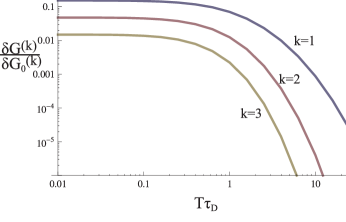
Figure 4: Temperature dependence of the first three harmonics of AB conductance for $g_{t}=500$, $g=30$, $N=10$, $\beta_{t}=1$ and $\tau_{D}/\tau_{RC}=120$.

4 Discussion

The results obtained here allow to formulate quantitative predictions regading the effect of electron-electron interactions on Aharonov-Bohm oscillations of conductance for a wide class of disordered nanorings embraced by our model. Of particular interest is the situation of large number of dots $N\gg 1$ which essentially mimics the behavior of diffusive nanostructures. In order to establish a direct relation to this important case it is instructive to introduce the diffusion coefficient $D=d^{2}/(2\tau_{D})$ and define the electron density of states $\nu=1/(d^{3}\delta)$, where $d$ is a linear dot size. Then we obtain with exponential accuracy:

$$\delta G^{(k)}\sim\left\{\begin{array}[]{lc}e^{-|k|(\mathcal{L}/\mathcal{L}_{\phi})}&\qquad\qquad T\ll D/(\mathcal{L}d),\\ e^{-|k|(\mathcal{L}/\mathcal{L}_{\phi})^{3/2}}&\qquad\qquad T\gg D/(\mathcal{L}d).\end{array}\right.$$

Here we introduced the ring perimeter $\mathcal{L}=Nd$ and the effective decoherence length

$$\mathcal{L}_{\phi}=\left\{\begin{array}[]{lc}\left(\frac{\pi\nu d^{3}D}{\ln\frac{4E_{C}}{\delta}}\right)^{1/2}&\qquad\qquad T\ll D/(\mathcal{L}d),\\ \left(\frac{12\nu d^{2}D^{2}}{T}\right)^{1/3}&\qquad\qquad T\gg D/(\mathcal{L}d).\end{array}\right.$$

Note in the high temperature limit $T\gg D/(\mathcal{L}d)$ the above results match with those derived earlier for metallic nanorings with the aid of different approaches [16, 17]. On the other hand, at lower $T$ our results are different. This difference is due to low temperature saturation of $\tau_{\phi}$ which was not accounted for in Refs. [16, 17]. A non-trivial feature predicted here is that – in contrast to weak localization [13] – the crossover from thermal to quantum dephasing is controlled by the ring perimeter $\mathcal{L}$. This is because only sufficiently long electron paths fully encircling the ring are sensitive to the magnetic flux and may contribute to AB oscillations of conductance.

We believe that the quantum dot rings considered here can be directly used for further experimental investigations of quantum coherence of interacting electrons in nanoscale conductors at low temperatures.

References

- [1] A.G. Aronov, Yu.V. Sharvin, Rev. Mod. Phys. 59 (1987) 755.
- [2] S. Chakravarty, A. Schmid, Phys. Rep. 140 (1986) 193.
- [3] D.S. Golubev, A.D. Zaikin, Phys. Rev. B 74 (2006) 245329.
- [4] D.S. Golubev, A.D. Zaikin, New J. Phys. 10 (2008) 063027.
- [5] D.S. Golubev, A.D. Zaikin, Physica E 40 (2007) 32.
- [6] A.G. Semenov, D.S. Golubev, A.D. Zaikin, Phys. Rev. B 79 (2009) 115302.
- [7] G. Schön, A.D. Zaikin, Phys. Rep. 198 (1990) 237.
- [8] S.V. Panyukov, A.D. Zaikin, Phys. Rev. Lett. 67 (1991) 3168.
- [9] Yu.V. Nazarov, Phys. Rev. Lett. 82 (1999) 1245.
- [10] D.S. Golubev, A.V. Galaktionov, A.D. Zaikin, Phys. Rev. B 72 (2005) 205417.
- [11] D.S. Golubev, A.D. Zaikin, Phys. Rev. Lett. 86 (2001) 4887; Phys. Rev. B 69 (2004) 075318.
- [12] D.A. Bagrets, Yu.V. Nazarov, Phys. Rev. Lett. 94 (2005) 056801.
- [13] D.S. Golubev, A.D. Zaikin, Phys. Rev. Lett. 81 (1998) 1074; Phys. Rev. B 59 (1999) 9195; Phys. Rev. B 62 (2000) 14061; Physica B 255 (1998) 164.
- [14] D.S. Golubev, A.D. Zaikin, J. Low Temp. Phys. 132 (2003) 11.
- [15] G.L. Ingold, Yu.V. Nazarov, Single Charge Tunneling, (Plenum Press, New York) NATO ASI Series B 294 (1992) p. 21.
- [16] C. Texier, G. Montambaux, Phys. Rev. B 72 (2005) 115327.
- [17] T. Ludwig, A.D. Mirlin, Phys. Rev. B 69 (2004) 193306.