Unidirectional Emission from Circular Dielectric Microresonators with a Point Scatterer

Abstract

Circular microresonators are micron sized dielectric disks embedded in material of lower refractive index. They possess modes of extremely high Q-factors (low lasing thresholds) which makes them ideal candidates for the realization of miniature laser sources. They have, however, the disadvantage of isotropic light emission caused by the rotational symmetry of the system. In order to obtain high directivity of the emission while retaining high Q-factors, we consider a microdisk with a pointlike scatterer placed off-center inside of the disk. We calculate the resulting resonant modes and show that some of them possess both of the desired characteristics. The emission is predominantly in the direction opposite to the scatterer. We show that classical ray optics is a useful guide to optimizing the design parameters of this system. We further find that exceptional points in the resonance spectrum influence how complex resonance wavenumbers change if system parameters are varied.

I Introduction

Thin dielectric microcavities of different shapes are widely used as microresonators in laser physics and integrated optics (see Vahala (2003); Ilchenko and Matsko (2006) and references therein). The new directions in microcavity laser research have been recently reviewed in Nosich et al. (2007). Microresonators are open systems coupled to the external world, and therefore do not have bound states. Instead, their eigenmodes (resonances) are characterized by complex wavenumbers $k=k_{r}+ik_{i}=\omega/c-i/(c\tau)$. Here $\tau$ is the lifetime of the resonance and $c$ denotes the speed of light. The so-called resonance quality factor ($Q$ factor for short) is then defined as $Q=k_{r}/2\,|k_{i}|$, and is a measure of the suitability of a mode for lasing.

The resonances of any passive (no active lasing particles) microcavity filled with nonmagnetic (${\bf B}={\bf H}$) dielectric material are the solutions of the time-independent Maxwell equations

$$\nabla\times{\bf E}=ik\,{\bf H},\quad\nabla\times{\bf H}=-ik\,\varepsilon\left({\bf r}\right){\bf E}$$ (1)

when appropriate boundary conditions on the fields $H$ and $E$ are imposed. When the fields are independent of $z$, which is strictly speaking only the case for a cylindrical microcavity of infinite length (see below), the above equations in cylindrical coordinates ($r,\varphi,z$) reduce to

$$\begin{split}\frac{1}{r}\frac{{\partial E_{z}}}{{\partial\varphi}}=ik\,H_{r},\quad-\frac{{\partial E_{z}}}{{\partial r}}=ik\,H_{\varphi},\\ \frac{1}{r}\left[{\frac{{\partial\left({rE_{\varphi}}\right)}}{{\partial r}}-\frac{{\partial E_{r}}}{{\partial\varphi}}}\right]=ik\,H_{z},\end{split}$$ (2)

and

$$\begin{split}\frac{1}{r}\frac{{\partial H_{z}}}{{\partial\varphi}}=-ik\,\varepsilon\left(r,\varphi\right)E_{r},\,\,\,\,-\frac{{\partial H_{z}}}{{\partial r}}=-ik\,\varepsilon\left(r,\varphi\right)E_{\varphi},\\ \frac{1}{r}\left[{\frac{{\partial\left({rH_{\varphi}}\right)}}{{\partial r}}-\frac{{\partial H_{r}}}{{\partial\varphi}}}\right]=-ik\,\varepsilon\left(r,\varphi\right)E_{z}.\end{split}$$ (3)

The solutions can be separated into TM waves ’transverse magnetic, i.e. $H_{z}=0$) and TE waves ‘transverse electric’, i.e. $E_{z}=0$). Introducing the position dependent refractive index $n(r,\varphi)\equiv\sqrt{\varepsilon(r,\varphi)}$, we get for TM modes a scalar wave equation for $E_{z}$,

$$\frac{{\partial^{2}E_{z}}}{{\partial r^{2}}}+\frac{1}{r}\frac{{\partial E_{z}}}{{\partial r}}+\frac{1}{{r^{2}}}\frac{{\partial^{2}E_{z}}}{{\partial\varphi^{2}}}+k^{2}n^{2}\left({r,\varphi}\right)E_{z}=0\,.$$ (4)

The magnetic field $H$ is then recovered from

$$H_{r}=-\displaystyle\frac{i}{{kr}}\frac{{\partial E_{z}}}{{\partial\varphi}},\quad H_{\varphi}=\frac{i}{{k\,}}\frac{{\partial E_{z}}}{{\partial r}}\,.$$ (5)

For TE modes, it is advantageous to introduce the new field $h_{z}(r,\varphi)\equiv H_{z}(r,\varphi)/n(r,\varphi)$. This field satisfies again a scalar wave equaton,

$$\frac{{\partial^{2}h_{z}}}{{\partial r^{2}}}+\frac{1}{r}\frac{{\partial h_{z}}}{{\partial r}}+\frac{1}{{r^{2}}}\frac{{\partial^{2}h_{z}}}{{\partial\varphi^{2}}}+k^{2}n^{2}(r,\varphi)\,h_{z}(r,\varphi)$$

$$+\left[\frac{\nabla^{2}n}{n(r,\varphi)}-2\left(\frac{\nabla n}{n(r,\varphi)}\right)^{2}\right]h_{z}(r,\varphi)=0\,,$$ (6)

and the electric field $E$ can be recovered in this case from

$$\begin{split}E_{r}=\frac{i}{{krn(r,\varphi)}}\left[{\frac{{\partial h_{z}}}{{\partial\varphi}}+\frac{1}{{\,n(r,\varphi)}}\frac{{\partial n}}{{\partial\varphi}}\,h_{z}(r,\varphi)}\right],\\ E_{\varphi}=-\frac{i}{{k\,n(r,\varphi)}}\left[{\frac{{\partial h_{z}}}{{\partial r}}+\frac{1}{{\,n(r,\varphi)}}\frac{{\partial n}}{{\partial r}}\,h_{z}(r,\varphi)}\right].\end{split}$$ (7)

The applicability of these equations can be extended from infinitely long cylindrical microcavities to flat microcavities for which the cavity thickness is only a fraction of the mode wavelength. The refractive index has then to be replaced by an effective refractive index $n_{{\rm eff}}(r,\varphi)$ which takes into account the material as well as the thickness of the cavity. We note that it is in general a difficult problem to explicitly compute $n_{{\rm eff}}(r,\varphi)$ for a given material and thickness (see, e.g., Ref. Lebental et al. (2007)), and one therefore typically resorts to using an experimentally determined effective refractive index instead.

The simplest microcavity shape is a thin circular microdisk. The technological progress in recent years has made possible the construction of microdisks in the $\mu$m-domain. They are natural candidates for the construction of lasers since some of their modes have extremely high $Q$-factor (low thresholds) McCall et al. (1992); Levi et al. (1993a). In those modes, which are called ‘whispering gallery modes’, light is trapped by total internal reflection and circulates along the circumference of the disk. As a consequence of the rotational symmetry the light emission of microdisks is isotropic. For many applications, however, a directional light emission is required. To obtain a directional emission we recently proposed to break the symmetry of a microdisk by placing a point scatterer inside but not at the center of the microdisk (see Ref. Dettmann et al. (2008a)). We have demonstrated that such a geometry leads to a significant enhancement of the directivity of some TM modes in outgoing light while preserving their high $Q$-factors. Other attempts to breaking the symmetry include the introduction of some other defects inside the microdisk like a linear defect Apalkov and Raikh (2004); Tulek and Vardeny (2007) or a hole Wiersig and Hentschel (2006). Another approach is to deform the boundary of the cavity Levi et al. (1993b); Nöckel et al. (1996); Lebental et al. (2006); Lee et al. (2007), or to couple light into and out of a microdisk with the aid of an optical fiber taper waveguide Srinivasan and Painter (2007). However, the advantage of our method is the analytic tractability which allows for a systematic optimization of the design parameters (location and strength of the scatterer) with only modest numerical efforts.

The purpose of this paper is to extend the theory in Dettmann et al. (2008a) to TE modes, and give a systematic study of the appearance of both highly directional TM and TE modes and its dependence on the distance of a point scatterer from the disk center. In particular, we provide arguments based on geometric optics to explain this dependence. This paper is organized as follows. In the following section, Sec. II, we use a Green’s function method to calculate the positions of the resonant modes of a microdisk with a point scatterer in the complex wavenumber plane. In Sec. III we discuss in some detail the physical interpretation of the parameter that describes the strength of the point scatterer. In Sec. IV we investigate in detail the directivity of the resonance modes for the microdisk with point scatterer, and in Sec. V we show that classical ray optics is a useful guide to optimizing the design parameters of the system. In Sec. VI we investigate the role of exceptional points in our system, and we finish with some concluding remarks in Sec. VII.

II Theory of Microdisk Cavities with a Point Scatterer

Let $\Psi$ stand for $E_{z}$ in the case of TM polarization and for $h_{z}$ in the case of TE polarization. For a homogeneous dielectric microdisk of radius $R$ and effective refractive index $n$ in a medium of refractive index $1$, Eqs. (4) and (6) take the form

$$\frac{{\partial^{2}\Psi}}{{\partial r^{2}}}+\frac{1}{r}\frac{{\partial\Psi}}{{\partial r}}+\frac{1}{{r^{2}}}\frac{{\partial^{2}\Psi}}{{\partial\varphi^{2}}}+k^{2}n^{2}\Psi\left({r,\varphi}\right)=0,$$ (8)

inside the microdisk ($r<R$) and the same form with $n$ replaced by $1$ outside the microdisk ($r>R$). The resonances are obtained by imposing outgoing boundary conditions at infinity, i.e. we require that $\Psi\left(r\right)\propto{{e^{ikr}}\mathord{\left/{\vphantom{{e^{ikr}}{\sqrt{r}}}}\right.\kern-1.2pt}{\sqrt{r}}}$, $r\rightarrow\infty$. Moreover, for physical reasons the value of the EM field at the disk center must be finite. At the boundary of the microdisk, $r=R$, the electric field component $E_{z}$ and its derivative has to be continuous for TM modes. Similarly, for TE modes, the field $h_{z}$ multiplied by the refractive index and its derivative divided by the refractive index has to be continuous at $r=R$. These boundary conditions lead to the ‘whispering gallery’ (WG) modes

$$\Psi^{m}=\left\{{\begin{array}[]{*{20}c}{N_{m}J_{m}\left({knr}\right)\left({\begin{array}[]{*{20}c}{\cos m\varphi}\\ {\sin m\varphi}\\ \end{array}}\right),\quad r<R,\vspace{8pt}}\\ {H_{m}\left({kr}\right)\left({\begin{array}[]{*{20}c}{\cos m\varphi}\\ {\sin m\varphi}\\ \end{array}}\right),\quad r>R,}\\ \end{array}}\right.$$ (9)

where for TM modes, the complex wavenumbers $k$ are solutions of

$$A_{m}^{\rm TM}\equiv J_{m}(knR)H_{m}^{\,\,\,{}^{\prime}}(kR)-n\,J_{m}^{\,\,\,{}^{\prime}}(knR)H_{m}(kR)=0,$$ (10)

and for TE modes, the complex wavenumbers $k$ are solutions of

$$A_{m}^{\rm TE}\equiv n\,J_{m}(knR)H_{m}^{\,\,\,{}^{\prime}}(kR)-J_{m}^{\,\,\,{}^{\prime}}(knR)H_{m}(kR)=0.$$ (11)

Here $J_{m}$ and $H_{m}$ are Bessel and Hankel functions of the first kind respectively, $m=0,1,2,...$ is the azimuthal modal index. The constants $N_{m}$ are given by

$$N_{m}=\begin{cases}H_{m}(kR)/J_{m}(knR)&\text{for TM modes}\\ H_{m}(kR)/(nJ_{m}(nkR))&\text{for TE modes}\,.\end{cases}$$ (12)

Physically, the azimuthal modal index $m=0,1,2,\ldots$ characterizes the field variation along the disk circumference, with the number of intensity hotspots being equal to $2m$. The wavenumbers, $k$, are twofold degenerate for $m>0$, and nondegenerate for $m=0$. The radial modal index $q=1,2,...$ will be used to label different resonances with the same azimuthal modal index $m$. For resonances which are relatively close to the real axis of the the complex wavenumber plane (so called ‘internal’ or ‘Feshbach’ resonances), the index $q$ gives in general the number of intensity spots in the radial direction. As discussed in detail in Dettmann et al. (2008b) there are exceptions to this rule for some TE internal resonances.

We note that for each fixed $m$, there exist further solutions of Eqs. (10,11) (so called ‘external’ or ‘shape’ resonances) which are typically located deeper in the lower half of the complex wavenumber planes compared to internal resonances (see Refs. Dubertrand et al. (2008); Ryu et al. (2008)). The external resonances are very leaky (low $Q$-factors) and, as a result, can not be directly used for lasing. However, they are of theoretical interest in their own right. To properly distinguish between external and internal resonances one needs to trace the resonances as a function of the refractive index $n$ to the values they obtain in the limit $n\rightarrow\infty$. As discussed in detail in Dettmann et al. (2008b) this limiting value is real for internal resonances, and complex (not real) for external resonances. The procedure of tracing the resonances in the complex wavenumber plane is especially important for TE modes for which some of the external resonances lie in the same domain of the complex wavenumber plane as the internal resonances. For an example of this phenomenon, we refer to Sec. IV.

In Dettmann et al. (2008a) we derived the Green’s function for the TM modes of a microdisk. Following Ref. Morse and Feshbach (1953) it is given by a sum over all angular harmonics $e^{\mathrm{i}m(\varphi-\varphi_{0})}$ multiplied by the corresponding radial parts. Using the same method it is not difficult to derive the Green’s function also for TE waves. In fact, both functions can be written as

$$G^{\text{TM/TE}}\left({{\bf r},{\bf r}_{0},k}\right)=\left\{{\begin{array}[]{*{20}c}{-\displaystyle\frac{\mathrm{i}}{4}H_{0}\left({kn\left|{{\bf r}-{\bf r}_{0}}\right|}\right)+\displaystyle\frac{\mathrm{i}}{4}\displaystyle\sum\limits_{m=0}^{\infty}{\displaystyle\frac{{C^{\text{TM/TE}}_{m}}}{{A^{\text{TM/TE}}_{m}}}\epsilon_{m}\cos\left[m\left({\varphi-\varphi_{0}}\right)\right]J_{m}\left({knr_{<}}\right)J_{m}\left({knr_{>}}\right)},}&{r_{<},r_{>}\,<\,R,}\\ {\displaystyle\frac{1}{2\pi kR}\displaystyle\sum\limits_{m=0}^{\infty}{\displaystyle\frac{1}{{A^{\text{TM/TE}}_{m}}}\epsilon_{m}\cos\left[m\left({\varphi-\varphi_{0}}\right)\right]J_{m}\left({knr_{<}}\right)H_{m}\left({kr_{>}}\right)},}&{r_{<}<R<r_{>},}\\ {-\displaystyle\frac{\mathrm{i}}{4}H_{0}\left({k\left|{{\bf r}-{\bf r}_{0}}\right|}\right)+\displaystyle\frac{\mathrm{i}}{4}\displaystyle\sum\limits_{m=0}^{\infty}{\displaystyle\frac{{B^{\text{TM/TE}}_{m}}}{{A^{\text{TM/TE}}_{m}}}\epsilon_{m}\cos\left[m\left({\varphi-\varphi_{0}}\right)\right]H_{m}\left({kr_{<}}\right)H_{m}\left({kr_{>}}\right)},}&{r_{<},r_{>}\,>\,R,}\\ \end{array}}\right.$$ (13)

where $r_{<}$ ($r_{>}$) is the smaller (larger) of $r$ and $r_{0}$. The coefficients are $\epsilon_{m}=2$ if $m\neq 0$, $\epsilon_{m}=1$ if $m=0$, and

$$\begin{split}B_{m}^{\rm TM}&=J_{m}\left({knR}\right)J_{m}^{\,\,\,{}^{\prime}}\left({kR}\right)-n\,J_{m}^{\,\,\,{}^{\prime}}\left({knR}\right)J_{m}\left({kR}\right),\\ C_{m}^{\rm TM}&=H_{m}\left({knR}\right)H_{m}^{\,\,\,{}^{\prime}}\left({kR}\right)-n\,H_{m}^{\,\,\,{}^{\prime}}\left({knR}\right)H_{m}\left({kR}\right),\\ B_{m}^{\rm TE}&=n\,J_{m}\left({knR}\right)J_{m}^{\,\,\,{}^{\prime}}\left({kR}\right)-J_{m}^{\,\,\,{}^{\prime}}\left({knR}\right)J_{m}\left({kR}\right),\\ C_{m}^{\rm TE}&=n\,H_{m}\left({knR}\right)H_{m}^{\,\,\,{}^{\prime}}\left({kR}\right)-H_{m}^{\,\,\,{}^{\prime}}\left({knR}\right)H_{m}\left({kR}\right).\end{split}$$

The resonances of the microdisk are then determined by the poles of the Green’s function i.e. by $A^{\text{TM/TE}}_{m}=0$. This agrees with resonance conditions (10) and (11). We note that the resonance wavefunctions are exponentially increasing as $r\rightarrow\infty$, and hence cannot be normalized. However any constant multiplying the resonance wavefunctions can be fixed by comparing the wavefunctions to the residues of the Green’s function.

Using methods of self-adjoint extension theory Zorbas (1980); Shigehara (1994), we showed in Ref. Dettmann et al. (2008a) that the presence of a point scatterer, which is located at a point ${\bf d}$ on the $x$-axis ($\varphi=0$), leaves the resonances of the unperturbed disk (WG modes) with the angular part $\sin(m\varphi)$ unchanged, while the complex wavenumbers $k_{\rm res}$ of the resonances with the angular part $\cos(m\varphi)$ become solutions of the transcendental equation

$$1-\lambda G_{\mathrm{reg}}({\bf d},{\bf d},k)=0\,.$$ (14)

Here $G_{\mathrm{reg}}$ is the regularized Green’s function which is obtained by subtracting the logarithmically divergent term $\ln(k_{0}|{\bf r}-{\bf r_{0}}|)/2\pi$ from the Green’s function (13) in the limit ${\bf r}$, ${\bf r_{0}}\rightarrow{\bf d}$. The two parameters $\lambda$ and $k_{0}$ can be absorbed in a single new parameter $a$ defined by $2\pi\equiv-\lambda\ln k_{0}a$. Then the condition for resonances (14) becomes

$$\begin{split}0=&-\frac{\mathrm{i}}{4}+\frac{{1}}{2\pi}\big{(}{\ln\frac{{k_{\,\rm{res}}na}}{{2}}+\gamma}\big{)}\\ &+\frac{\mathrm{i}}{4}\sum_{m=0}^{\infty}{\frac{C_{m}(k_{\rm res})}{A_{m}(k_{\rm res})}}\,\epsilon_{m}{J^{2}_{m}\left({k_{\,\rm{res}}nd}\right)}\,,\end{split}$$ (15)

where $\gamma\approx 0.5772$ is the Euler-Mascheroni constant. The parameter $a$ then determines the “strength” of the point scatterer located at the distance $d=|{\bf d}|<R$ from the center.

The corresponding resonance wavefunction is given by

$$\Psi({\bf r})=NG({\bf r},{\bf d},k_{\rm res})\,,$$ (16)

where $G$ is the Green’s function in Eq. (13), and $N$ is a normalization factor. Outside of the microdisk, i.e. in the region $r>R$, the field takes the form

$$\Psi=\frac{N}{{2\pi k_{\rm res}R}}\sum\limits_{m=0}^{\infty}{\frac{{\epsilon_{m}\cos\left(m{\varphi}\right)J_{m}\left({k_{\rm res}nd}\right)}}{{A_{m}}}}H_{m}\left({k_{\rm res}r}\right).$$ (17)

In principle, the normalization factor can be obtained again from the residue of the Green’s function of the perturbed system (see Eq. (19) in the next section).

From Eq. (15) we see that in the limit $a=0$ and $a\rightarrow\infty$ we recover the resonances of the unperturbed microdisk (without a point scatterer). For $a$ close to 0 or infinity, the approximate solutions of Eq. (15) can be found perturbatively. In leading order one finds

$$k_{{\rm res}}\cong k-{\mathrm{i}}\,\pi\frac{{C_{m}(k)\,}}{{D_{m}(k)\,}}\frac{{\epsilon_{m}J_{m}^{2}\left({knd}\right)}}{{2R\ln a}}\,,$$ (18)

where $D_{m}=(\mathrm{d}A_{m}/\mathrm{d}k)/R$ is given by

$$\begin{split}D_{m}^{{\rm TM}}&=J_{m}(knR)H_{m}^{\,\,{}^{\prime\prime}}(kR)-n^{2}J_{m}^{\,\,{}^{\prime\prime}}(knR)H_{m}(kR),\\ D_{m}^{{\rm TE}}&=n\left[J_{m}(knR)H_{m}^{\,\,{}^{\prime\prime}}(kR)-J_{m}^{\,\,{}^{\prime\prime}}(knR)H_{m}(kR)\right]\\ &\qquad+(n^{2}-1)\,\,J_{m}^{\,\,{}^{\prime}}(knR)H_{m}^{\,\,{}^{\prime}}(kR),\end{split}$$

and $k$ is a resonance wavenumber of the unperturbed disk, with azimuthal modal index $m$.

III Relation to a Finite Size Scatterer

Before we investigate the solutions of Eq. (15) and the corresponding resonance wave functions numerically, let us discuss the physical interpretation of the parameter $a$. This parameter can be related to that of a small but finite size scatterer as long as this scatterer can be treated in the $s$-wave approximation. The Green’s function of the system with a point scatterer follows from self-adjoint extension theory Zorbas (1980); Shigehara (1994), and is given by

$$G^{a}({\bf r},{\bf r_{0}},k)=G({\bf r},{\bf r_{0}},k)+\frac{G({\bf r},{\bf d},k){\cal D}G({\bf d},{\bf r_{0}},k)}{1-{\cal D}G^{\mathrm{sc}}({\bf d},{\bf d},k)}\;.$$ (19)

Here $G^{\mathrm{sc}}({\bf d},{\bf d},k)$ is the Green’s function in (13) for both arguments less than $R$ and without the term $-\mathrm{i}H_{0}(nk|{\bf r}-{\bf r}_{0}|)/4$ (i.e. without the free Green’s function). The quantity ${\cal D}$ is the so-called diffraction coefficient

$${\cal D}=\frac{2\pi}{\mathrm{i}\pi/2-\gamma-\log(nka/2)}\;.$$ (20)

One can easily check that the resonance wavenumbers in (15) coincide with the poles of the Green’s function (19).

The form of the Green’s function in (19) is identical to that of a system perturbed by a small $s$-wave scatterer within the Geometrical Theory of Diffraction Keller (1962); Vattay et al. (1994). The optical theorem imposes a restriction on the diffraction coefficient given by $|{\cal D}|^{2}=-4\operatorname{Im}{\cal D}$ if $k\in\mathbb{R}$. It is a consequence of the conservation of energy. The condition for ${\cal D}$ is equivalent to $\operatorname{Im}{\cal D}^{-1}=1/4$. In order to find a physical interpretation for the parameter $a$ one has to compare the diffraction coefficient (20) with that of a small but finite size scatterer in the $s$-wave approximation. In fact, our parameter $a$ was chosen in such a way that the coefficient (20) agrees with that of a small $s$-wave scatterer of radius $a$ with Dirichlet boundary conditions $\Psi=0$ along its circumference (see Rosenqvist et al. (1996)).

Let us now perturb the microdisk by a small hole of radius $b$ placed at a distance $d$ from the center, and filled with a material of refractive index $n_{b}$. The diffraction coefficient depends only on local properties near the perturbation and can be obtained from the Green’s function for a small circular disk of radius $b$ with refractive index $n_{b}$ embedded within material of refractive index $n$ (i.e. one can neglect the outside region with refractive index 1). But this Green’s function can be obtained in exactly the same manner as the Green’s function in Eq. (13). The only differences are the corresponding radius and the refractive indices. In particular, the new coefficients are

$$\begin{split}{\cal A}_{m}^{\rm TM}&=n\,J_{m}(kn_{b}R)H_{m}^{\,\,\,{}^{\prime}}(knR)-n_{b}\,J_{m}^{\,\,\,{}^{\prime}}(kn_{b}R)H_{m}(nkR),\\ {\cal A}_{m}^{\rm TE}&=n_{b}\,J_{m}(kn_{b}R)H_{m}^{\,\,\,{}^{\prime}}(knR)-n\,J_{m}^{\,\,\,{}^{\prime}}(kn_{b}R)H_{m}(nkR),\\ {\cal B}_{m}^{\rm TM}&=n\,J_{m}(kn_{b}R)J_{m}^{\,\,\,{}^{\prime}}(knR)-n_{b}\,J_{m}^{\,\,\,{}^{\prime}}(kn_{b}R)J_{m}(nkR),\\ {\cal B}_{m}^{\rm TE}&=n_{b}\,J_{m}(kn_{b}R)J_{m}^{\,\,\,{}^{\prime}}(knR)-n\,J_{m}^{\,\,\,{}^{\prime}}(kn_{b}R)J_{m}(nkR).\end{split}$$

We are interested in the Green’s function outside the small disk. If that disk is small enough to be treated in the $s$-wave approximation we need to keep only the term $m=0$ in the sum over modal indices

$$G^{b}({\bf r},{\bf r_{0}},k) =-\frac{\mathrm{i}}{4}H_{0}(kn|{\bf r}-{\bf r_{0}}|)$$

$$\qquad+\frac{\mathrm{i}}{4}\frac{{\cal B}_{0}}{{\cal A}_{0}}H_{0}(kn|{\bf r}|)H_{0}(kn|{\bf r_{0}}|)\,.$$ (21)

This function has the form of (19) with $G({\bf r},{\bf r_{0}},k)=-\mathrm{i}H_{0}(kn|{\bf r}-{\bf r_{0}}|)/4$, $G^{\mathrm{sc}}({\bf r},{\bf r_{0}},k)=0$, and we can read off the diffraction coefficient as ${\cal D}=-4\mathrm{i}{\cal B}_{0}/{\cal A}_{0}$. One can check that the optical theorem is satisfied. Using the asymptotic forms of Bessel and Hankel functions for small arguments, we obtain that ${\cal D}^{-1}\approx\mathrm{i}/4-[\pi b^{2}k^{2}(n_{b}^{2}-n^{2})]^{-1}$. The comparison with the diffraction coefficient for a point scatterer (20) gives the condition on the parameter $a$ of the point scatterer for modelling the finite size scatterer

$$\ln\frac{nka}{2}+\gamma\approx\frac{2}{b^{2}k^{2}(n_{b}^{2}-n^{2})}\;.$$ (22)

In this equation $k$ is real, i.e. its imaginary part which is small for resonances with high $Q$ factor is neglected. Finally, we should note that the $s$-wave approximation itself is valid if the small but finite size scatterer is located not too close to the circumference of the disk, i.e. for $|nk(R-d)|\gg 1$, and if

$$\frac{{\cal A}_{0}}{{\cal B}_{0}}\ll\frac{{\cal A}_{1}}{{\cal B}_{1}}\;.$$ (23)

IV Far Field Directivity

In order to quantify the far-field behavior of the field $\Psi$ we consider its asymptotics for $r\rightarrow\infty$ which has the form

$$\Psi\left({\bf r},k_{{\rm res}}\right)=\Psi\left(r,\varphi,k_{{\rm res}}\right)\propto\frac{{\exp(ik_{{\rm res}}r)}}{{\sqrt{r}}}f\left(\varphi\right).$$ (24)

Then, the directionality of the emission can be characterized with the directivity $D$ which is defined as the ratio of the power emitted into the main beam direction $\varphi_{\text{max}}$ to the total power averaged over all possible directions,

$$D=\frac{2\pi\,|f_{{\rm max}}(\varphi_{{\rm max}})|^{2}}{{\int\limits_{0}^{2\pi}{\left|{f(\varphi)}\right|^{2}d\varphi}}}\,.$$ (25)

Note that the resonances of the disk without a scatterer have $D=1$ for $m=0$ and $D=2$ for $m\neq 0$.

For the disk with a point scatterer, we investigate the level dynamics of the resonances as a function of the parameter $a$ by numerically solving Eq. (15) for TM and TE modes, respectively. As mentioned in Sec. II and discussed in more detail in Dettmann et al. (2008a), the perturbed resonances reduce to the unperturbed resonances (microdisk without scatterer) in the limits $a\to 0$ and $a\to\infty$. The wavenumbers of the perturbed disk thus evolve a long line segments in the complex wavenumber plane which start and end at unperturbed resonances when $a$ is varied from 0 to infinity. In our numerical procedure which consists of a Newton method to solve Eq. (15) we vary $a$ from $10^{-30}$ to $10^{\,30}$ and use Eq. (18) to obtain starting points for the numerics in these limits. For each resonance wavenumber found this way, the corresponding wavefunction is obtained from Eq. (16). In particular, in the outside region the wavefunction takes the form of (17) from which we can compute the directivity $D$.

In fact, because of the relation between wavefunction and the Green’s function (16) we can formally associate a directivity $D$ to any point in the complex $kR$ plane (for a fixed choice of ${\bf d}$). This directivity has only a direct physical interpretation if the $kR$ value corresponds to a resonance of the disk with a point scatterer. For general $k$, $D(k)$ is rather a characterization of the Green’s function (13). It is helpful to consider also this formal directivity because it enables one to clearly identify the regions in the $kR$ plane where a perturbation of the circular disk by a scatterer (at position ${\bf d}$) should lead to highly directional modes.

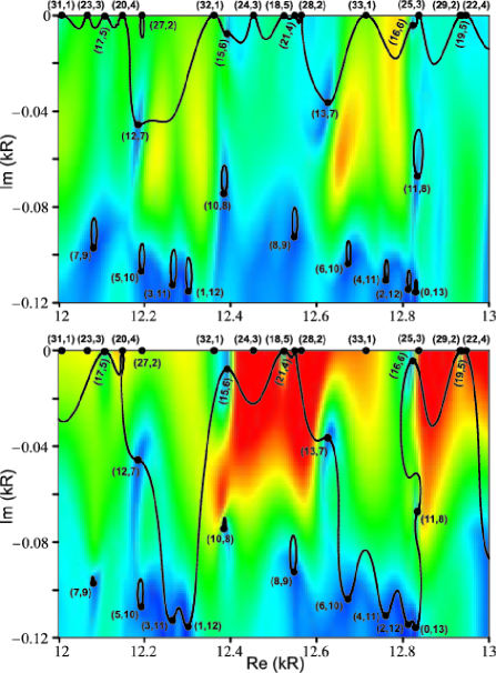
Figure 1: (color online). Level dynamics (black curves) of the TM resonances in the complex wave number plane for a dielectric disk with $n=3.0$ and $R=1.0\,\mu$m and a point scatterer of varying coupling parameter $a$. The solid circles mark the unperturbed resonances with azimuthal and radial modal indices $(m,q)$. For the upper panel the scatterer is placed at distance $d=0.9$ $\mu\text{m}$ from the centre, for the lower panel $d=0.5$ $\mu$m. The color code in the $kR$ plane indicates the directivity $D$ of the emission as explained in the text (blue marks small values of $D$, red marks high values of $D$).

As a first example, we study the level dynamics of TM resonances in the range $12<{\rm Re}(kR)<13$ for a disk of effective refractive index $n=3.0$ and radius $R=1\,\mu$m (these parameters are close to the ones in Ref. Peter et al. (2005)) with a point scatterer placed at two different distances ($d=0.9\,\mu$m and $d=0.5\,\mu$m) from the center of the disk. The results are shown in Fig. 1. The background color in Fig. 1 indicates the directivity $D$ for any point of the $kR$ plane computed as mentioned above. Low values of $D$ correspond to the color blue, and high values of $D$ correspond to deep red. Superimposing the curves of the wavenumber level dynamics we can immediately see in which region of the $kR$ plane the highly directional modes are located.

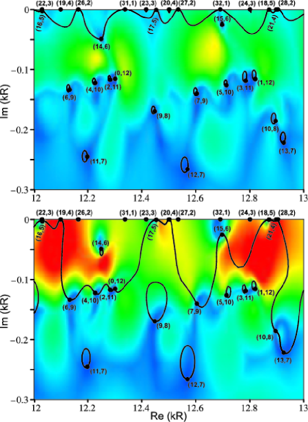
Figure 2: (color online). Analogue of Fig. 1 for TE resonances. The parameters are the same as in Fig. 1.

Figure 2 shows the corresponding plot for TE modes in the same parameter range as in Figure 1. Like in the case of TM polarization there are highly directional TE modes for a wide range of $Q$-factors. From the figures one sees that for both TM and TE resonant modes, placing the point scatterer at a distance $d=0.5\,\mu$m from the center yields a better directivity than for $d=0.9\,\mu$m. We will explain this observation in Sec. V. The directivity reaches values as high as $D\approx 15$ for some specific TM modes and $D\approx 13$ for some specific TE modes.

Figure 3: The far-field intensities of the unperturbed TM resonance with modal indices $(21,4)$ (thin curve), and of the highly directional TM resonance (thick curve) that is obtained from the unperturbed mode by perturbing a dielectric disk with $n=3.0$ and $R=1.0\,\mu$m with a point scatterer of strength $a=10^{-6}$ placed at distance $d=0.5\,\mu$m from the disk center.

Figure 4: The field intensity in the far-field of the unperturbed TE resonance with modal indices $(21,4)$ (thin curve), and of the highly directional TE resonance (thick curve) that is obtained from the unperturbed mode by perturbing a dielectric disk with $n=3.0$ and $R=1.0\,\mu$m with a point scatterer of strength $a=10^{-6}$ placed at distance $d=0.5\,\mu$m from the disk center.

In Fig. 3 we show the field intensity at the distance $r=500~{}\mu$m (far-field region) for a highly directional TM resonance mode which is obtained by a small perturbation of the unperturbed TM resonance mode with modal indices $(21,4)$. It has directivity ($D\cong 13$) and complex wavenumber $kR=12.54929-{\mathrm{i}}\,0.000045$, and is compared to the unperturbed mode with directivity $D=2$ and complex wavenumber $kR=12.54876-{\mathrm{i}}\,0.000001$. The highly directional mode is obtained from the unperturbed mode if a very weak point scatterer of strength $a\cong 10^{-6}$ is placed at a distance $d=0.5\,\mu$m from the centre of the disk. Indeed, we expect this from Fig. 1, because the unperturbed mode lies in a highly red region in the $kR$ plane where a small perturbation should lead to a highly directional mode. According to Eq. (22) the perturbation is comparable to that of a finite size scatterer of radius $b\approx 0.01\mu m$ and refractive index $n_{b}=1$.

In Fig. 4 we show the far field intensity of the analogous TE mode. It is again obtained by a perturbation of the mode $(21,4)$ of the circular disk by placing a point scatterer of strength $a\cong 10^{-6}$ at distance $d=0.5\,\mu$m from the centre of the disk. For this polarization the unperturbed mode $(21,4)$ is located at $kR=12.90089-{\mathrm{i}}\,0.000001$ in the complex wave number plane while the perturbed mode is located at $kR=12.90187-{\mathrm{i}}\,0.000087$. Their directivities are $D=2$ and $D\cong 11$ respectively. Both of the above highly directional modes are good candidates for lasing since their $Q$-factors are large. In fact, $Q\approx 1.4\cdot 10^{5}$ for the highly directional TM resonance and $Q\approx 7.4\cdot 10^{4}$ for the highly directional TE resonance. Moreover, they have unidirectional emission at an angular direction of 180 degrees.

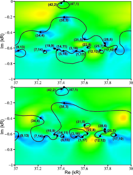
Figure 5: (color online). Level dynamics of the TM resonances in the complex wave number plane for a dielectric disk with $n=1.4$ and $R=10.51$ mm and a point scatterer of varying coupling parameter $a$. The solid circles mark the unperturbed resonances with azimuthal and radial modal indices $(m,q)$. For the upper panel the scatterer is placed at distance $d=9.585$ mm from the centre, for the lower panel $d=9.385$ mm. As before, the color code indicates the directivity $D$ of the emission.

As a second example, we study the level dynamics of TM and TE resonances in the range $37<{\rm Re}(kR)<38$ for a disk of effective refractive index $n=1.4$ and radius $R=10.51$ mm (these parameters are close to the ones of the experimental setup of Schwefel and Preu, Schwefel and Preu (2008)) with a point scatterer placed at two close distances $d=9.585$ mm and $d=9.385$ mm from the centre of the disk, see figs. 5 and 6. From these two figures one can see that even a relatively small change in the position of a point scatterer can lead to a significant change in the level dynamics. The directivity of some perturbed TM modes reaches values as high as $D\cong 10$ for a point scatterer located at $d=9.385$ mm, see the lower panel of Fig. 5, and the directivity of some TE modes reaches values as high as $D\cong 8$ for a point scatterer located at $d=9.585$ mm, see the upper panel of Fig. 6. In general, however, the directivity is lower than for $n=3$ in Figs. 1 and 2. This will be explained in the next section.

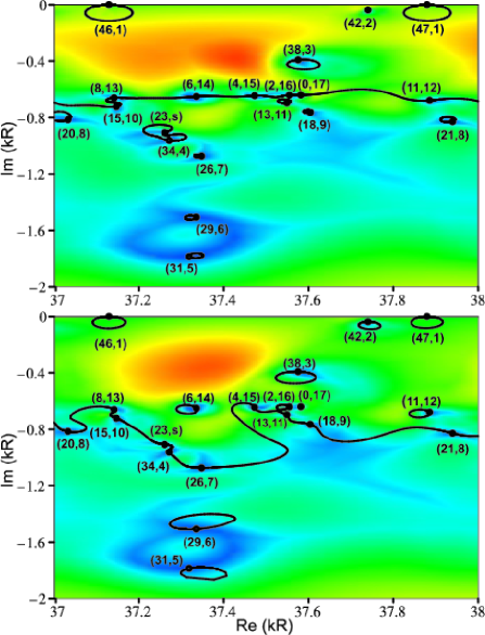
Figure 6: (color online). Analogue of Fig. 5 for TE resonances. The parameters are the same as in Fig. 5. The label $(23,s)$ indicates a shape resonance with azimuthal model index $m=23$.

Another interesting feature is the appearance of the unperturbed shape (external) TE resonance denoted by $(23,s)$ in Fig. 6 which is located in the region of the complex wave number plane where one would expect to have internal resonances only. This is related to a peculiar behaviour of some of the unperturbed external TE resonances that was observed in Ref. Dettmann et al. (2008b). For large refractive indices $n$, the external resonances are located much deeper in the complex wavenumber plane than the internal resonance. This clear separation by the magnitude of the imaginary part of the wavenumbers ceases to exist for small $n$ in the case of TE modes where some external resonances mix with the internal resonances. The wavefunctions of such external resonances acquire similar features as the wavefunctions of internal resonances. In particular they can spoil the interpretation of the radial modal index $q$ as the number of peaks of the wavefunction in the radial direction (see Dettmann et al. (2008b)) for internal resonances with the same azimuthal modal index. Furthermore for the disk with a point scatterer, the external resonance (23, s) in Fig. 6 illustrates the fact that unperturbed external resonances also serve as starting and end points of the line segments that result from the level dynamics of perturbed resonances in the complex wavenumber plane upon varying $a$ from 0 to $\infty$.

Figure 7: The far-field intensities ($r=5000$ mm) of the unperturbed TM resonance with $kR=37.599462-{\mathrm{i}}\,0.488553$, $m=31$, $q=5$ (thin curve), and of the highly directional perturbed TM resonance with $kR=37.621007-{\mathrm{i}}\,0.523645$, $d=9.385$ mm, $a\cong 0.07$ (thick curve) in a dielectric disk with $n=1.4$ and $R=10.51$ mm.

Figure 8: The far-field intensities ($r=5000$ mm) of the unperturbed TE resonance with $kR=37.129055-{\mathrm{i}}\,0.000177$, $m=46$, $q=1$ (thin curve), and of the directional perturbed TE resonance with $kR=37.142373-{\mathrm{i}}\,0.001832$, $d=9.585$ mm, $a\cong 4\cdot 10^{-5}$ (thick curve) in a dielectric disk with $n=1.4$ and $R=10.51$ mm.

In Fig. 7 we show the field intensities at the distance $r=5000$ mm (far-field region) for the unperturbed resonant TM mode with modal indices $(31,5)$, complex wavenumber $kR=37.599462-{\mathrm{i}}\,0.488553$, and directivity $D=2$ as well as for the highly directional ($D\cong 10$) TM resonant mode with complex wavenumber $kR=37.621007-{\mathrm{i}}\,0.523645$. The unperturbed mode $(31,5)$ transforms to the highly directional mode with the above complex wavenumber if we place a point scatterer of strength $a\cong 0.07$ at distance $d=9.385$ mm from the centre of the disk. We note that despite of the high directivity this mode is not suitable for lasing because it has only a small $Q$ factor of about $36$.

In Fig. 8 we show the field intensities at the distance $r=5000$ mm (far-field region) for the unperturbed resonant TE mode with modal indices $(46,1)$, complex wavenumber $kR=37.129055-{\mathrm{i}}\,0.000177$, and directivity $D=2$ as well as for the directional ($D\cong 6$) TE resonant mode with complex wavenumber $kR=37.142373-{\mathrm{i}}\,0.001832$. The unperturbed mode $(46,1)$ transforms to the directional mode with the above complex wavenumber if we place a point scatterer of strength $a\cong 4\cdot 10^{-5}$ at distance $d=9.585$ mm from the centre of the disk. This mode has $Q\cong 10^{4}$ and, therefore, is suitable for lasing.

V Directivity and Geometric Optics

To systematically study the appearance of highly directional modes, we calculate the average directivity for a region in the complex wavenumber plane as a function of the distance, $d$, of the point scatterer from the center. To this end we define the average directivity

$$D_{{\rm av}}=\frac{1}{\Delta k_{r}\Delta k_{i}}\int_{k_{r}^{-}}^{k_{r}^{+}}\text{d}k_{r}\int_{k_{i}^{-}}^{k_{i}^{+}}\text{d}k_{i}\,{D\left(k\right)}\,,$$ (26)

where $[k^{-}_{r},k^{+}_{r}]\times[k^{-}_{i},k^{+}_{i}]$ is a rectangular region in the complex wavenumber plane of side lengths $\Delta k_{r}=k^{+}_{r}-k^{-}_{r}$ and $\Delta k_{i}=k^{+}_{i}-k^{-}_{i}$ . Note that the integration is over all $k$ in the rectangular region where $D\left(k\right)$ is formally defined using formulas (17), (24), and (25), for general $k$ rather than just for the resonant $k_{\rm res}$ (see Sec. IV). In Figs. 9 and 10. we show $D_{{\rm av}}$ computed for the region $12<{\rm Re}(kR)<13$, $-0.1<{\rm Im}(kR)<0$ as a function of $d$ for four microdisks of radius $R=1\,\mu$m and effective refractive indices of $n=3.0$, $n=2.6$, $n=2.25$, and $n=1.4$, and for the region $37<{\rm Re}(kR)<38$, $-1<{\rm Im}(kR)<0$ for four disks of radius $R=10.51\,$mm with the same effective refractive indices, respectively.

Figure 9: The average directivity, $D_{{\rm av}}$, of TM (thick curves) and TE (thin curves) polarized light in the range $12<{\rm Re}(kR)<13$, $-0.1<{\rm Im}(kR)<0.0$ for each position, $d$, of a point scatterer in microdisks of radius $R=1\,\mu$m and various effective refractive indices as shown.

Figure 10: The average directivity, $D_{{\rm av}}$, of TM (thick curves) and TE (thin curves) polarized light in the range $37<{\rm Re}(kR)<38$, $-1<{\rm Im}(kR)<0.0$ for each position, $d$, of a point scatterer in microdisks of radius $R=10.51\,\mu$m and various effective refractive indices as shown.

Remarkably, a rough approximation of the values for $d$ which lead to high $D_{{\rm av}}$ can be found from geometric optics. To this end let us consider parallel rays that come in from infinity and enter a dielectric disk of radius $R$ and effective refractive index $n$. There is one ray which goes through the center of the disk, the central ray. The rays that are infinitesimally close to this central ray will cross the central ray at the point with distance

$$d_{o}=\frac{R}{n-1}$$ (27)

to the center of the disk located on the opposite side of the center of the disk. So, conversely, putting a point scatterer at this focal point leads to a strongly directional light emission in the an angular direction of 180^∘ which also agrees with the observation in the previous section.

The value of $d_{o}$ is indicated by the vertical lines in Figs. 9 and Fig. 10. One can see that in most cases $d_{o}$ is close to the optimal value range for the point scatterer positions in the figures. Taking into account the finite size of the disk, we note that formula (27) is valid only for refractive indices greater than $2$. For smaller refractive indexes the optimal position should be as close as possible to the boundary of the disk.

VI Exceptional points

The line segments that connect unperturbed resonances as the parameter $a$ varies from zero to infinity can change considerably if the distance, $d$, of the point scatterer to the center is changed. This can be seen already in Figures 5 and 6 which are for two different but close values of $d$. The connections between the unperturbed resonances are very different there, i.e. the line segments connect different unperturbed resonances if $d$ is varied only slightly. In the present section we want to look at this in more detail.

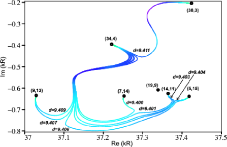
Figure 11: (color online). Level dynamics of the TM resonances in the complex wave number plane for a dielectric disk with $n=1.4$ and $R=10.51$mm and a point scatterer of varying coupling parameter $a$ for several positions $d$ of the scatterer. All start from the unperturbed resonance $(34,4)$. The solid circles mark the unperturbed resonances with modal indices $(m,q)$. The color code indicates the directivity $D$ of the emission (green marks small values of $D$, red marks high values of $D$).

As a first example we investigate the perturbation of one particular resonance of the microdisc. We choose the TM resonance with modal indices $(34,4)$ of the dielectric disk with $n=1.4$ and $R=10.51$. We then place a point scatterer at distance $d$ from the center of the disk. For different values of $d$ we vary the strength of the scatterer $a$ from $0$ to infinity. This yields a family of line segments in the complex wavenumber plane which all start at the unperturbed resonance $(34,4)$ but, depending on $d$, end at different unperturbed resonances. This is shown in Fig. 11. It is remarkable that the connections between the different unperturbed resonances depend so sensitively on the value of $d$. In the small range from $d=9.400$ to $d=9.411$ shown in Fig. 11 the unperturbed resonance $(34,4)$ is connected to five different unperturbed resonances.

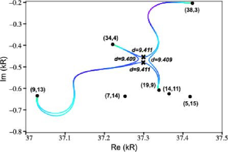
Figure 12: (color online). Level dynamics of the TM resonances in the complex wave number plane for a dielectric disk with $n=1.4$ and $R=10.51$mm and a point scatterer of varying coupling parameter $a$ for two positions $d$ of the scatterer. The solid circles mark the unperturbed resonances with azimuthal and radial modal indices $(m,q)$. As the position of the scatterer changes from $d=9.409$ to $d=9.411$ the connections of the unperturbed resonances change.

Next we investigate how the connections are rearranged. The connections between the unperturbed resonances can only change upon variation of $d$ if for one value of $d$ different line segments intersect tangentially at a point in the complex $kR$-plane. This point corresponds to a degenerate resonance. This mechanism is illustrated in Fig. 12. For $d=9.409$ the resonance $(34,4)$ is connected to the resonance $(9,13)$, while the resonance $(19,9)$ is connected to $(38,3)$. For the value $d=9.411$ the connections have changed. The resonance $(34,4)$ is now connected to $(38,3)$, while $(19,9)$ is connected to $(9,13)$. Although not shown in the figure, there is a value of $d$ for which two line segments touch each other at a point at which two perturbed resonances coallesce and become degenerate.

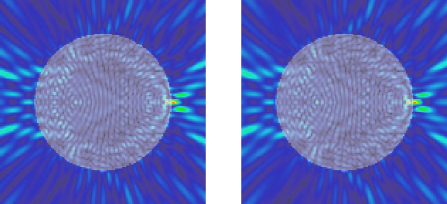
Figure 13: (color online). Two almost degenerate TM resonance states for a dielectric disk with $n=1.4$ and $R=10.51$mm. The corresponding wavenumbers are shown by crosses in Fig. 12.

For an open system like the dielectric disk degeneracies are generically of a special type which are called exceptional points Heiss (2000); Kato (1966). Exceptional points can be observed if at least two real-valued parameters of a non-hermitian operator are varied. In our case the non-hermitian operator is the differential operator acting on $\Psi$ in Eq. (8) which is non-hermitian due to the outgoing boundary condition. The two real parameters are the parameters $a$ and $d$. At an exceptional point two (or more) eigenvalues of the non-hermitian operator coallesce, and the corresponding eigenstates become identical. The pair of eigenstates which becomes degenerate at an exceptional point also show a characteristic behavior if the two parameters are changed along a closed loop about the exceptional points. Smoothly following the pair of eigenstates from a starting point of the loop upon one full traversal of the loop yields a pair of eigenstates in which the eigenstates started with are swapped and in which one member of the pair has a reversed sign. Exceptional points have recently received a lot of attention. For an example in the field of microlasers and more references see Ref. J. Wiersig (2008).

Figure 14: Far field of the two resonance states shown by crosses in Fig. 12.

To illustrate the coalescence of resonance states that is typical for exceptional points we show in Fig. 13 the fields of the two almost degenerate resonances marked in Fig. 12. Fig. 14 shows the corresponding far-field behaviour.

The numerical results in this section indicate that exceptional points are quite common for dielectric disks with point scatterers. They control the connections between the unperturbed resonances and can be easily found by noting when these connections change upon varying the position ${\bf d}$ of the scatterer.

VII Conclusion

We have shown that perturbations of a dielectric disk by a point scatterer can lead to highly directional resonance modes with large Q-factors. This is demonstrated in particular by the unidirectional modes in Figs. 3 and 4. To obtain modes with these properties is one of the main goals in the design of dielectric microcavities.

The system studied has the advantage that it is relatively simple and can be treated to a large extent analytically by a Green’s function method. This allows for a systematic investigation of the system over a large parameter range with only moderate numerical effort. We found that several numerical results can be understood with the help of a simple geometrical optics model. This model helps to find the optimal position of the scatterer, it explains why the directivity is in general higher for refractive index $n=3$ than for $n=1.4$, and also why the emission occurs predominantly in a direction opposite of the position of the point scatterer. It also suggests future investigation of an elliptical microcavity with a scatterer at one of the foci and refractive index inverse to the eccentricity, as in that case focusing in geometric optics is exact, i.e. the paraxial approximation is not required Boriskin et al. (2004).

The Green’s function method also allows one to associate a directivity with different regions of the complex $kR$ plane. This is very useful because it indicates in which regions of the $kR$ plane one can expect highly directional modes if one perturbs the dielectric disk by the scatterer. It would be helpful to find a semiclassical explanation for the dependence of the directivity on the wavenumber $k$.

Most interesting for applications we also discussed how the system studied can be realized physically by a small but finite sized scatterer. This connection can be made as long as the scatterer can be treated in the $s$-wave approximation, and is found to be valid for examples with high Q-factor and directivity. An important open question is how the directivity and $Q$-factor depend on the size and shape of a larger scatterer when corrections to the $s$-wave approximation are taken into account.

References

- Vahala (2003) K. Vahala, Nature 424, 839 (2003).
- Ilchenko and Matsko (2006) V. S. Ilchenko and A. B. Matsko, IEEE Journal of Selected Topics in Quantum Electronics 12, 15 (2006).
- Nosich et al. (2007) A. I. Nosich, E. I. Smotrova, S. V. Boriskina, T. M. Benson, and P. Sewell, Opt. Quant. Electron. 39, 1253 (2007).
- Lebental et al. (2007) M. Lebental, N. Djellali, C. Arnaud, J.-S. Lauret, J. Zyss, R. Dubertrand, C. Schmit, and E. Bogomolny, Phys. Rev. A 76, 023830 (2007).
- McCall et al. (1992) S. L. McCall, A. F. J. Levi, R. E. Slusher, S. J. Pearton, and R. A. Logan, Appl. Phys. Lett. 60, 289 (1992).
- Levi et al. (1993a) A. F. J. Levi, R. E. Slusher, S. L. McCall, S. J. Pearton, and R. A. Logan, Appl. Phys. Lett. 63, 1310 (1993a).
- Dettmann et al. (2008a) C. P. Dettmann, G. V. Morozov, M. Sieber, and H. Waalkens, Europhys. Lett. 82, 34002 (2008a).
- Apalkov and Raikh (2004) V. M. Apalkov and M. E. Raikh, Phys. Rev. B 70, 195317 (2004).
- Tulek and Vardeny (2007) A. Tulek and Z. V. Vardeny, Appl. Phys. Lett. 90, 161106 (2007).
- Wiersig and Hentschel (2006) J. Wiersig and M. Hentschel, Phys. Rev. A 73, 031802(R) (2006).
- Levi et al. (1993b) A. F. J. Levi, R. E. Slusher, S. L. McCall, J. L. Glass, S. J. Pearton, and R. A. Logan, Appl. Phys. Lett. 62, 561 (1993b).
- Nöckel et al. (1996) J. U. Nöckel, A. D. Stone, G. Chen, H. L. Grossman, and R. K. Chang, Opt. Lett. 21, 1609 (1996).
- Lebental et al. (2006) M. Lebental, J. S. Lauret, R. Hierle, and J. Zyss, Appl. Phys. Lett. 88, 031108 (2006).
- Lee et al. (2007) S. B. Lee, J. Yang, S. Moon, J. H. Lee, K. An, J. B. Shim, H. W. Lee, and S. W. Kim, Appl. Phys. Lett. 90, 041106 (2007).
- Srinivasan and Painter (2007) K. Srinivasan and O. Painter, Phys. Rev. A 75, 023814 (2007).
- Dettmann et al. (2008b) C. P. Dettmann, G. V. Morozov, M. Sieber, and H. Waalkens (2008b), arXiv:0903.5333.
- Dubertrand et al. (2008) R. Dubertrand, E. Bogomolny, N. Djellali, M. Lebental, and C. Schmit, Phys. Rev. A 77, 013804 (2008).
- Ryu et al. (2008) J.-W. Ryu, S. Rim, Y.-J. Park, C.-M. Kim, and S.-Y. Lee, Phys. Lett. A 372, 3531 (2008).
- Morse and Feshbach (1953) P. M. Morse and H. Feshbach, Methods of Theoretical Physics, Part I (McGraw-Hill, New York, 1953).
- Zorbas (1980) J. Zorbas, J. Math. Phys. 21, 840 (1980).
- Shigehara (1994) T. Shigehara, Phys. Rev. E 50, 4357 (1994).
- Keller (1962) J. B. Keller, J. Opt. Soc. Am. 52, 116 (1962).
- Vattay et al. (1994) G. Vattay, A. Wirzba, and P. E. Rosenqvist, Phys. Rev. Lett. 73, 2304 (1994).
- Rosenqvist et al. (1996) P. Rosenqvist, N. D. Whelan, and A. Wirzba, J. Phys. A 29, 5441 (1996).
- Peter et al. (2005) E. Peter, P. Senellart, D. Martrou, A. Lemaître, J. Hours, J. M. Gérard, and J. Bloch, Phys. Rev. Lett. 95, 067401 (2005).
- Schwefel and Preu (2008) H. Schwefel and S. Preu, private communication (2008).
- Heiss (2000) W. D. Heiss, Phys. Rev. E 61, 929 (2000).
- Kato (1966) T. Kato, Perturbation Theory of Linear Operators (Springer, Berlin, 1966).
- J. Wiersig (2008) M. H. J. Wiersig, S. W. Kim, Phys. Rev. A 78, 053809 (2008).
- Boriskin et al. (2004) A. V. Boriskin, A. I. Nosich, S. V. Boriskina, T. M. Benson, P. Sewell, and A. Altintas, Microw. Opt. Technol. Lett. 43, 515 (2004).