Quantum oscillations from Fermi arcs

Abstract

When a metal is subjected to strong magnetic field $B$ nearly all measurable quantities exhibit oscillations periodic in $1/B$. Such quantum oscillations represent a canonical probe of the defining aspect of a metal, its Fermi surface (FS). In this study we establish a new mechanism for quantum oscillations which requires only finite segments of a FS to exist. Oscillations periodic in $1/B$ occur if the FS segments are terminated by a pairing gap. Our results reconcile the recent breakthrough experiments showing quantum oscillations in a cuprate superconductor YBa₂Cu₃O_6.51, with a well-established result of many angle resolved photoemission (ARPES) studies which consistently indicate “Fermi arcs” – truncated segments of a Fermi surface – in the normal state of the cuprates.

In conventional metals superconductivity can be understood as a pairing instability of the Fermi surface bcs . Recent unambiguous identification of Shubnikov - de Haas taillefer1 ; bangura1 and de Haas - van Alphenjaudet1 oscillations in YBa₂Cu₃O_6.51 (YBCO) in high magnetic fields ushered a new era in the field by furnishing a long awaited proof that a Fermi surface exists in a high-temperature superconductor (SC). This important discovery, which according to the conventional paradigm implies a closed Fermi surface (FS), creates interesting new puzzles. The existence of such a closed FS contradicts the well-established result of many angle resolved photoemission (ARPES) studies which consistently indicate “Fermi arcs” – truncated segments of a Fermi surface – in the normal state of cupratesding1 ; kanigel1 ; shen1 . In this theoretical study we establish a new mechanism for quantum oscillations which requires only finite segments of the FS to exist. We present arguments that this new mechanism is relevant to the cuprates and show that it accounts for the quantum oscillations in a model that exhibits genuine Fermi arcs terminated by a pairing gap, consistent with the ARPES data.

Quantum oscillation experiments in YBCO taillefer1 ; bangura1 ; jaudet1 , when analyzed using the conventional Onsager-Lifshitz picture onsager1 ; lifshitz1 ; shoenberg1 , indicate small Fermi pockets each with an area covering approximately 1.9% of the first Brillouin zone (BZ). Such small Fermi pockets do not arise naturally from the band structure calculations and their total area is inconsistent with the nominal doping concentration. To explain these results proposals for various states with broken translational symmetry have been put forward millis1 ; kee1 ; rice1 ; sachdev-galitski ; podolski , leading to complicated band structures with multiple Fermi pockets. One would, however, expect to see signatures of such a Fermi surface reconstruction in other experiments, most notably the ARPES, which is capable of mapping out Fermi surfaces of metals with high accuracy. Yet, extensive ARPES studies on various cuprate materials show no evidence for Fermi pockets.

One can attempt to reconcile the quantum oscillation data with ARPES by postulating that Fermi pockets do exist but cannot be seen by ARPES for various reasons. Of these, the suppression of the photoemission intensity on the pocket’s back side due to the coherence factors is often citedstanescu .

In this study we adopt a radically different point of view – we assume that the Fermi arcs observed in ARPES are real and ask if such genuine Fermi arcs can give rise to quantum oscillations. With one additional experimentally motivated assumption norman3 , namely that the gap terminating the arcs is of the pairing origin, we find the answer to be affirmative. Our reasoning that underlies this conclusion is a natural extension of the conventional Onsager-Lifshitz picture supplemented by the analysis of what happens once the electron reaches the arc endpoint. These semiclassical considerations are then supplemented and confirmed by exact numerical diagonalizations of a fully quantum lattice model.

In what follows we advance two principal ideas. First, we formulate a simple, experimentally motivated model for a normal state of underdoped cuprate superconductors that exhibits genuine Fermi arcs terminated by a pairing gap. Second, we demonstrate that in an applied external magnetic field the low-energy density of states (DOS) in this model oscillates as a function of energy as well as magnetic field. The DOS is periodic in energy with frequency that is linear in $1/B$ and proportional to the Fermi arc length. At the Fermi level (or any other fixed low energy) the DOS oscillates with $1/B$. The frequency of oscillations is not related to any area in momentum space; instead it is proportional to the gap amplitude and the fraction of the FS that is gapped. The origin of the quantum oscillations in our model is the periodic appearance of low energy Andreev-type bound statesadagideli associated with the fermi arcs and is distinct from all mechanisms proposed to explain quantum oscillations in cuprates in the existing literaturemillis1 ; kee1 ; rice1 ; sachdev-galitski ; podolski ; varma ; vafek .

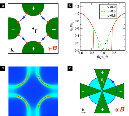
Figure 1: The Fermi-arc metal. a) The gap structure of the Fermi arc metal (FAM) in the shaded areas adjacent to the BZ faces the gap is nonzero while the excitations in the rest of the BZ are gapless. Blue lines represent the gapless segments of the Fermi surface known as the ‘Fermi arcs’. When a perpendicular magnetic field $B$ is applied to the system electrons in the gapless regions follow semiclassical orbits which coincide with contours of constant energy $\epsilon_{\bf k}$. b) The amplitude of the modified $d$-wave gap $\tilde{\Delta}_{\bf k}$, Eq. (2), with $\tau=0.01$ plotted along the line connecting points $(0,\pi)$ and $(\pi,0)$ of the BZ. c) Spectral intensity, $A({\bf k},\omega)=-\pi^{-1}{\rm Im}G({\bf k},\omega)$, of the Fermi-arc metal at $\omega=0$. Here $G({\bf k},\omega)=[\omega-\epsilon_{\bf k}+i\Gamma-\tilde{\Delta}_{\bf k}^{2}/(\omega+\epsilon_{\bf k}+i\Gamma)]^{-1}$ is the Green’s function of Hamiltonian (3), with additional impurity broadening represented by $\Gamma=25$meV. We use the tight-binding parametrization for $\epsilon_{\bf k}$ of Ref. norman0, and $\Delta_{0}=50$meV, $\nu=0.6$ and $\tau=0.01$. d) Simplified model of FAM with circular Fermi surface and piecewise constant gap used in semiclassical analysis. We denote the angular extent of the arcs and gapped regions as $\theta_{a}$ and $\theta_{g}=\pi/2-\theta_{a}$ respectively.

I Fermi-arc metal

We now provide a justification for the above claims. Our starting point is a simple phenomenological model for the ‘Fermi-arc metal’ (FAM) that we take to describe the non-superconducting state of underdoped cuprates with the quasiparticle excitation spectrum adiabatically connected to the ordinary $d$-wave superconductor. The latter is well-known to describe the superconducting ground state of cuprates. It has a pairing gap $\Delta_{\bf k}=\Delta_{0}\chi_{\bf k}$ with $\chi_{\bf k}={1\over 2}(\cos k_{x}-\cos k_{y})$ and quasiparticle excitation spectrum

$$E_{\bf k}=\sqrt{\epsilon_{\bf k}^{2}+\Delta_{\bf k}^{2}},$$ (1)

with $\epsilon_{\bf k}$ the band dispersion referenced to the Fermi level $\epsilon_{F}$. We assume that the excitations of the Fermi-arc metal have the same BCS form as Eq. (1) but with $\Delta_{\bf k}$ replaced by a modified $d$-wave gap $\tilde{\Delta}_{\bf k}$ which vanishes along the BZ diagonals as illustrated in Fig. 1a. Although the detailed form of $\tilde{\Delta}_{\bf k}$ is unimportant for the subsequent discussion we often find it useful to parameterize it as

$$\tilde{\Delta}_{\bf k}=\Delta_{0}{\chi_{\bf k}\over e^{(\nu^{2}-\chi_{\bf k}^{2})/\tau^{2}}+1}.$$ (2)

Here $\nu$ sets the length of the arc while $\tau$ controls the width of the step between the large-gap and zero-gap regions as illustrated in Fig. 1b. The ordinary $d$-wave superconductor is recovered in the limit $\nu,\tau\to 0$.

Several remarks are in order before we address quantum oscillations in this model. (i) We think of the above postulated Fermi-arc metal spectrum as originating from a BCS-type pairing Hamiltonian

$${\cal H}=\sum_{{\bf k}\sigma}\epsilon_{\bf k}c^{\dagger}_{{\bf k}\sigma}c_{{\bf k}\sigma}+\sum_{{\bf k}}(\tilde{\Delta}_{\bf k}\ c^{\dagger}_{{\bf k}\uparrow}c^{\dagger}_{-{\bf k}\downarrow}+{\rm h.c.})$$ (3)

where $c^{\dagger}_{{\bf k}\sigma}$ creates an electron with momentum ${\bf k}$ and spin $\sigma$. Although the microscopic Hamiltonian that would stabilize the mean-field state described by Eqs. (2,3) is presently not known, we see no fundamental reason why such a state could not occur for suitably chosen electron-electron interaction. We remark that Fermi arcs have been argued to appear in a phase-fluctuating SC fm1 ; altman1 and various more exotic quantum states such as the “algebraic charge liquid” kaul1 . (ii) A system described by Hamiltonian (3) would in fact be a superconductor, albeit with low superfluid density due to ungapped portions of the Fermi surface. We thus view this BCS Hamiltonian as an effective mean-field theory valid on intermediate length scales; at long length scales (compared to the magnetic length) phase fluctuations disrupt long-range superconducting order and render the system normal. (iii) The motivation for our phenomenological model comes primarily from experimental considerations. Indeed many experimental studies hint at the existence of the residual superconducting order in the pseudogap state uemura1 ; corson1 ; pasler1 ; ong1 ; ong2 ; lem1 . A Bogoliubov-type dispersion of quasiparticles in cuprates above $T_{c}$, observed very recently by ARPES norman3 , provides further direct evidence for the pairing nature of the pseudogap. The spectral intensity computed from our model and displayed in Fig. 1c is in detailed agreement with this data. Finally, (iv) we note that within the space of mean-field models the above construction appears to be the only way to construct genuine Fermi arcs. As mentioned above, particle-hole instabilities without exception produce closed Fermi surfaces which can only terminate at BZ boundaries.

II Semiclassical analysis

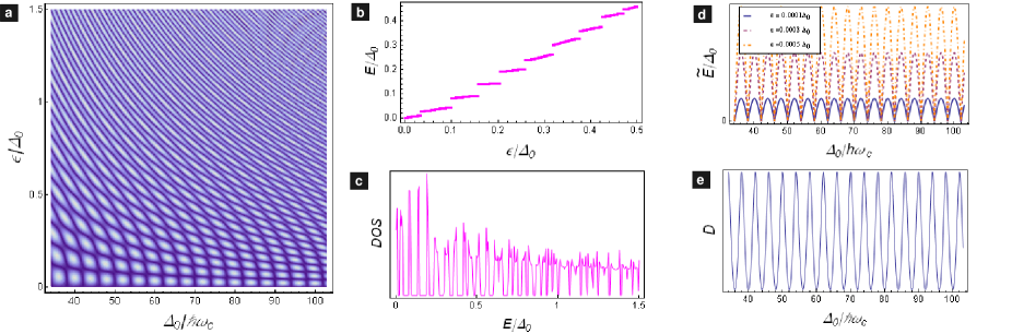
Figure 2: Semiclassical analysis. a) Density plot of the quasi-energy $\tilde{E}$ as a function of the inverse magnetic field (times $\Delta_{0}m_{c}c/e$) and the band energy (in units of the gap amplitude). $\tilde{E}$ is analytically obtained for the simplified Fermi-arc metal with a piecewise constant gap structure; it is scaled by $\hbar\omega_{c}$ and ranges between 0 (dark) and 1 (bright). b) Quasiparticle excitation energy, $E$, in the Fermi-arc metal as a function of the band energy $\epsilon$ at constant $B$. The quasi-particle energy is related to the quasi-energy $\tilde{E}$ as $E=\tilde{E}+n\hbar\omega_{c}$, where $n$, the unwinding index, is chosen to continuously match $E$ with $\epsilon$ for $\epsilon\gg\Delta_{0}$, and maintain $E$ as a piecewise continuous and monotonically increasing function of $\epsilon$. c) Density of states at a constant magnetic field $B\approx 40$T as a function of energy. d) The quasi-energy, $\tilde{E}$, for several low lying states with $\epsilon<\hbar\omega_{c}$ vs. $1/B$. e) The density of states at the Fermi energy vs. the magnetic field. In both plots the given field range corresponds to $20-60$T. The number of DOS oscillations found in this range is about 17, in good agreement with the experiments. In all panels $\theta_{a}=\pi/4$ corresponding to $\nu\sim 0.6$ in the numerical study.

In the absence of a gap, the classical equations of motion for an electron wave packet are

$$\hbar\dot{{\bf k}}=-{e\over c}({\bf v}_{\bf k}\times{\bf B}),\ \ \ \ \dot{{\bf r}}={\bf v}_{\bf k}={1\over\hbar}\nabla_{{\bf k}}\epsilon_{{\bf k}}.$$ (4)

Eqs. (4) imply that the electrons move on constant energy contours in momentum space. The time it takes to complete a cycle is $T=2\pi/\omega_{c}$ with $\omega_{c}=eB/m_{c}c$ the cyclotron frequency.

When constructing a wave packet to describe the semiclassical motion in the FAM, clearly the motion on the arcs is governed by Eq. (4). However, the evolution in momentum space drives the wave packet into the gapped region where its charge is no longer a good quantum number due to electron-hole mixing induced by the pairing gap. We therefore choose to construct our semiclassical wave packet out of ‘bogolons’ rather than electrons. These are Bogoliubov-de Gennes (BdG) quasiparticles of the underlying superconductor and can be thought of as coherent mixtures of electrons and holes. The bogolon wavefunction $\Psi_{\bf k}=(u_{{\bf k}},v_{{\bf k}})$ is an eigenstate of the BdG Hamiltonian

$${\cal H}_{\bf k}=\begin{pmatrix}\epsilon_{\bf k}&\tilde{\Delta}_{\bf k}\\ \tilde{\Delta}_{\bf k}&-\epsilon_{\bf k}\end{pmatrix}=\epsilon_{\bf k}\sigma_{3}+\Delta_{\bf k}\sigma_{1},$$ (5)

where $\sigma_{j}$ are the Pauli matrices acting in the particle-hole space.

The momentum ${{\bf k}}$ of the bogolon wavepacket continues to evolve according to Eq. (4) since both the velocity ${\bf v}_{{\bf k}}$ and the charge $e$ have opposite signs for the particle and the hole components. The real-space motion, however, is sensitive to the particle-hole mixing since the particle and the hole move in opposite directions. This leads to a modified real-space equation of motion

$$\dot{{\bf r}}=(|u_{{\bf k}}|^{2}-|v_{{\bf k}}|^{2}){\bf v}_{\bf k},$$ (6)

which represents the net center of mass motion of the bogolon wavepacket.

The semiclassical approximation amounts to introducing periodic time dependence in the Hamiltonian, in lieu of the magnetic field: ${\cal H}(t+T)={\cal H}(t)\equiv{\cal H}_{{\bf k}(t)}$. Unlike in the gapless case where ${\cal H}(t)=$const, here ${\cal H}(t)$ exhibits time dependence due to the momentum-dependent gap $\Delta(t)=\tilde{\Delta}_{{\bf k}(t)}$, while $\epsilon=\epsilon_{\bf k}$ remains a constant of motion. To find the solution of the time-dependent Schrödinger equation,

$$i\hbar\dot{\Psi}={\cal H}(t)\Psi,$$ (7)

we employ the Floquet theoremstockmann , which is the analog of the familiar Bloch theorem for time-periodic Hamiltonians; it states that solutions of Eq. (7) have the form $\Psi(t)=e^{-i\tilde{E}t/\hbar}f_{E}(t)$ with $f_{E}(t+T)=f_{E}(t)$. Here $e^{-i\tilde{E}T/\hbar}$ and $f_{E}(T)$ are the eigenvalue and the eigenstate, respectively, of the Floquet operator

$${\cal F}={\cal T}\exp\left[{-i\over\hbar}\int_{0}^{T}{\cal H}(t)dt\right],$$ (8)

and ${\cal T}$ represents the time-ordering operator. If we regard the two-component structure of $\Psi(t)$ as a pseudospin, then the Floquet states precess about a time dependent axis $\epsilon{\bf\hat{z}}+\Delta(t){\bf\hat{x}}$.

The quantity $\tilde{E}$ has dimensions of energy and is closely related to the quasiparticle energy of the original time-independent problem. Since the Floquet equation yields $e^{-i\tilde{E}T/\hbar}$ and $T=2\pi/\omega_{c}$ it is clear that $\tilde{E}$ is defined only modulo $\hbar\omega_{c}$. This is analogous to momentum being defined only modulo reciprocal lattice vectors in the Bloch theory. Henceforth we refer to $\tilde{E}$ as ‘quasi-energy’.

In order to obtain analytic results we simplify our model further. We assume a free-electron dispersion $\epsilon_{\bf k}=\hbar^{2}k^{2}/2m-\epsilon_{F}$ and that the FAM gap is piecewise constant and dependent only on the momentum direction. We take $\tilde{\Delta}_{\bf k}$ equal to zero on the arcs and $\pm\Delta_{0}$ elsewhere as illustrated in Fig. 1d. The details of the calculation of the Floquet quasi-energy are provided in the Methods. Here we present the results and discuss their implications.

The quasi-energy as a function of both the band energy $\epsilon$ and the magnetic field is shown in Fig. 2a. It contains most of the physics of this model. Fig. 2b shows a cut along the $\epsilon$ direction for constant $B$. The quasiparticle energy dispersion is obtained by a simple ‘unwinding’ procedure, described in Methods. Energy bands separated by small gaps result, in close analogy to the Bloch energy bands. The density of states in Fig. 2c displays clear periodic structure with frequency that can be estimated from Eq. (16) as

$$F_{\epsilon}={\theta_{a}\over\pi\hbar\omega_{c}}.$$ (9)

This is in agreement with the exact numerical results which are discussed in the next section.

We now turn our attention to the low-energy behavior of the FAM as a function of field $B$. Near the Fermi energy, $\epsilon\rightarrow 0$, the quasi-energy coincides with the quasi-particle energy, $E=\tilde{E}$, and no unwinding is necessary. When $\epsilon\to 0$ the quasi-energy vanishes, but the density of states, which is proportional to $dE/d\epsilon$, depends strongly on the magnetic field. In Fig. 2d we present the quasi-energy for a few different values of $\epsilon$ close to the Fermi energy as a function of $1/B$. In certain magnetic fields the density of lines is high and this translates to the sharp peaks in the DOS shown in Fig. 2e . This result is directly related to the experimentally observed oscillations. From Eq. (16) we may deduce that a peak in the Fermi energy DOS occurs whenever $\cos(\Delta_{0}\theta_{g}/\hbar\omega_{c})=0$, leading to oscillation frequency

$$F=\Delta_{0}{\theta_{g}m_{c}\over\pi\hbar e}.$$ (10)

Using $\Delta_{0}=80$meV, $\theta_{g}=\pi/4$ (Ref. damascelli1, ) and a cyclotron mass $m_{c}=3m_{e}$ (Ref. bangura1, ) we estimate $F=518$T, very close to the dominant experimental frequency 530-540T in YBCO.

Some intuitive understanding of the origin of the DOS oscillations can be gained by examining a typical low-energy Floquet state $f_{E}(t)$ and its associated real-space trajectory. This is illustrated in Fig. 3. The states contributing to high DOS are reminiscent of the Andreev bound states found on extended impurities and on sample edges in $d$-wave superconductorsadagideli . The periodicity in inverse magnetic field in this model is a consequence of the periodic appearance of these Andreev-type states on the Fermi arcs at low energies.

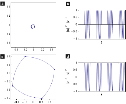
Figure 3: Semiclassical trajectories. Left column: Sample real-space trajectories. Right column: the quasi-particle group velocity relative to $v_{F}$, $|u|^{2}-|v|^{2}$, as a function of time along the trajectory. When $\epsilon\ll\Delta_{0}$ the bogolon pseudospin lies in the $y-z$ plane. Its projection on the $z$ axis is $|u|^{2}-|v|^{2}$. The states contributing to high DOS [panels (a) and (b) with $\hbar\omega_{c}={\Delta_{0}\theta_{g}/(4+{1\over 2})\pi}$] have their pseudospin pointing in the $y$-direction on the arc and are precessing in the $y-z$ plane in the gapped region. This means that on the arc the state is a perfect mixture of a particle and a hole, resembling a familiar Andreev bound state. The associated real-space trajectory encloses a particularly small area, since on the arc, the group velocity vanishes, $|u|^{2}-|v|^{2}=0$. On the other hand, the states near the DOS minimum [panels (c) and (d), $\hbar\omega_{c}={\Delta_{0}\theta_{g}/4\pi}$], point in the $z$ pseudo-spin direction and are thus either particles or holes. Their motion is dominated by the arc region, and the real-space trajectory encloses a large area. The DOS oscillations with $B$ may be understood as follows. In order to exhibit no real-space motion on the arc, Andreev states must point in the $y$ pseudospin direction. In the gapped region, the pseudospin precesses about the $x$-axis (assuming $\epsilon\ll\Delta_{0}$). If the magnetic field is such that the time to traverse the gapped region, $\theta_{g}/\omega_{c}$, allows exactly an integer plus one half cycles, the pseudospin will end up in the $-y$ direction and will continue to have zero motion on the next arc, thus giving a consistent Floquet state.

The quantum oscillation mechanism described above is dominant for quasiparticle energies much smaller than the gap amplitude $\Delta_{0}$, and does not involve the conventional Onsager-Lifshitz action considerations. Obviously, the action must be considered to obtain the normal-metal behavior in the limit of small gap or large arcs. The interplay of the two mechanisms then becomes complicated and we briefly discuss it in Methods.

III Lattice model

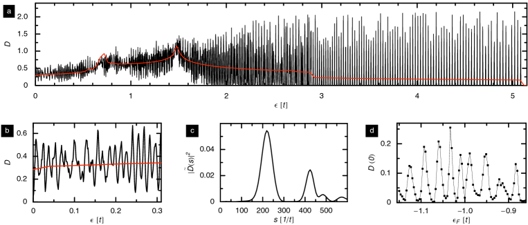
Figure 4: Exact diagonalization of the lattice model. a) DOS as a function of energy in the Fermi-arc metal in zero (red) and non-zero (black) magnetic field corresponding to two vortices in a $20\times 20$ magnetic unit cell. In YBCO with lattice constant $a_{0}\simeq 4$Å this corresponds to the physical field of about 64T. The parameters used are as follows, $\Delta_{0}/t=1$, $\epsilon_{F}/t=-1.3$, $\nu=0.6$ and $\tau=0.1$. b) The low-energy DOS for the same parameters, in detail. c) The power spectrum of the low-energy DOS showing dominant frequency of oscillations $210t^{-1}$ and its second harmonic. d) DOS at the Fermi level as a function of $\epsilon_{F}$.

In order to exemplify the validity of our semiclassical analysis we now consider a fully quantum-mechanical lattice model of the Fermi-arc metal and confirm the existence of quantum oscillations by exact numerical calculations. To this end, we study the real-space version of the Hamiltonian (3),

$${\cal H}=\sum_{ij\sigma}t_{ij}e^{i\theta_{ij}}c^{\dagger}_{i\sigma}c_{j\sigma}+\sum_{ij}\left[\tilde{\Delta}({\bf r}_{i},{\bf r}_{j})\ c^{\dagger}_{i\uparrow}c^{\dagger}_{j\downarrow}+{\rm h.c.}\right],$$ (11)

where $c^{\dagger}_{i\sigma}$ creates an electron with spin $\sigma$ at site ${\bf r}_{i}$ of the square lattice. The effect of magnetic field is described by the usual Peierls factors $\theta_{ij}=(2\pi/\Phi_{0})\int_{{\bf r}_{i}}^{{\bf r}_{j}}{\bf A}\cdot{\bf dl}$ and the SC order parameter $\tilde{\Delta}({\bf r}_{i},{\bf r}_{j})$ is correspondingly taken to contain a periodic lattice of Abrikosov vortices. This is achieved by adopting

$$\tilde{\Delta}({\bf r}_{1},{\bf r}_{2})=e^{i\Theta({\bf R})}\sum_{\bf k}e^{i{\bf r}\cdot{\bf k}}\tilde{\Delta}_{\bf k},$$ (12)

where ${\bf R}=({\bf r}_{1}+{\bf r}_{2})/2$ is the center of mass and ${\bf r}={\bf r}_{1}-{\bf r}_{2}$ the relative coordinate of the Cooper pair. The vortex lattice is reflected in the phase $\Theta({\bf R})$ winding by $2\pi$ around each vortex while the Fermi-arc structure in $k$-space follows from taking $\tilde{\Delta}_{\bf k}$ as described by Eq. (2). In order to keep subsequent calculations simple we limit ourselves to the nearest-neighbor electron hopping in the kinetic term: $t_{ii}=\epsilon_{F}$, $t_{ij}=-t$ for $(i,j)$ nearest neighbors and $t_{ij}=0$ otherwise.

We solve the problem posed by Eqs. (11,12) by employing the Franz-Tesanovic (FT) transformationft1 . This unitary transformation removes the non-trivial phase $\Theta({\bf R})$ from the pairing term and renders the transformed Hamiltonian translationally invariant with a unit cell containing two superconducting vortices. Eigenstates of this new Hamiltonian then can be conveniently found by appealing to the Bloch theorem. Ref. vft1, gives a detailed description of the implementation of the FT transformation to the lattice model of $s$-, $p$- and $d$-wave superconductors. The treatment of our modified $d$-wave SC follows as a straightforward generalization of this procedure.

The results of our numerical calculations are summarized in Fig. 4. The density of states $D(\epsilon)$ of the modified $d$-wave SC in the applied magnetic field shows the expected Landau level structurevft1 at energies exceeding about $3\Delta_{0}$. The surprising new result is the appearance of a clear periodic structure in $D(\epsilon)$ even at low energies inside the SC gap. This is unlike the ordinary $d$-wave SC where the Landau level type oscillations are known to be absent at low energies ft1 ; vft1 ; kita1 ; marinelli1 (we have confirmed this result by setting $\nu=0$ in our model). We attribute the low-energy oscillations to the gapless regions of the BZ implied by the modified $d$-wave order parameter Eq. (2) with $\nu\neq 0$.

The power spectrum of the low-energy DOS displayed in Fig. 4c confirms the periodic structure with a period that scales with $1/B$, in accordance with the semiclassical result Eq. (9). Physical observables, such as the specific heat and resistivity, depend on DOS at the Fermi level, $D(\epsilon_{F})$. Fig. 4d shows that $D(\epsilon_{F})$ exhibits similar oscillatory behavior.

The above exact numerical results show unambiguous evidence for quantum oscillations in FAM, a system that by construction exhibits genuine Fermi arcs terminated by a pairing gap. Although the exact diagonalization technique does not allow us to study these oscillations as a function of smoothly varying field $B$ (and thus compare directly to experiment), we have verified that oscillations in the energy variable are in qualitative as well as semi-quantitative agreement with the semiclassical picture presented in Sec. II. Specifically, we have analyzed the dependence of oscillation frequency $s$ on the gap amplitude $\Delta_{0}$ and the arc length $\nu$ and found these in agreement with the semiclassical predictions. This comparison is discussed more fully in the Methods.

IV Outlook

The original observation of quantum oscillations in YBCO taillefer1 has been interpreted as quantitatively consistent with the ARPES measurements shen1 by assuming that the Fermi arc observed in ARPES was a part of a Fermi pocket resulting from the Fermi surface reconstruction due to a symmetry breaking instability with wavevector $(\pi,\pi)$. Such a Fermi pocket would have an area of about 2% of the BZ, consistent with the observed oscillation frequency. The ARPES data used for this comparison however pertain not to YBCO but to a different high-$T_{c}$ compound Na_2-xCa_xCu₂O₂Cl₂ (NaCCOC). If one uses instead the ARPES data on YBCO that became available more recently damascelli1 , then the agreement disappears: the corresponding Fermi pocket would comprise about $5\%$ of the BZ, leading to the frequency more than twice that observed in experiment. The two experiments are easily reconciled by appealing to the Fermi arc picture advocated above, where the frequency of oscillations does not relate to any Fermi surface area but originates from the periodic appearance of Andreev-type states associated with Fermi arcs. The oscillation frequency (10) depends on the gap amplitude and the size of the gapped region in the Fermi-arc metal.

The above comparison illustrates some key differences between the conventional Onsager-Lifshitz picture of quantum oscillations in YBCO millis1 ; kee1 ; rice1 and the mechanism invoking genuine Fermi arcs terminated by a pairing gap proposed in this study. The latter relies only on the FS structure that is directly seen in ARPES while the former must make assumptions about unseen portions of the FS in the parts of the BZ where the ARPES indicates a large gapmillis1 ; kee1 ; rice1 . A direct observation of Fermi arcs at low temperatures in high magnetic fields would discriminate between the two pictures. Under such conditions ARPES experiments are not feasible but it should be possible to image the FS by means of the scanning tunneling probe using the technique of Fourier-transform interference spectroscopy hoffman1 ; mcelroy1 ; tami1 . Even if confirmed, the microscopic origin of the Fermi arc phenomenon remains an open question, the answer to which may pave the road towards the full solution of the cuprate mystery.

V Acknowledgments

The authors acknowledge illuminating discussions with D. Bonn, W. Hardy, B. Seradjeh, L. Taillefer, Z. Tesanovic, O. Vafek, M. Vojta and N-C. Yeh. The work was supported in part by NSERC, CIfAR (MF), DFG through SFB 608 (HW), the Packard Foundation, and the Research Corporation (GR).

VI Methods

VI.1 Experimental considerations

A crucial assumption we made in deducing the oscillatory behavior of $D(\epsilon)$ in Eqs. (9,10) is that the gap structure itself is field-independent. This is equivalent to assuming that magnetic field enters the underlying mean-field Hamiltonian via the usual minimum substitution but does not alter any of its parameters. This known to be true in ordinary metals but it is less obvious that this assumption applies to our Fermi-arc metal which relies on the existence of the residual SC gap. The amplitude and the $k$-space structure of the latter could be susceptible to magnetic field. Specifically, if the Fermi arc length depended on $B$ then the frequency of the quantum oscillations would itself become a function of $B$, in contradiction to experimental finding of constant frequency. Since there exist no independent measures of the Fermi arc length as a function of $B$, and since the microscopic theory underlying the Fermi arc phenomenon is also unknown, we must adopt the arc length independence on $B$ in the experimentally relevant interval 20-60T as an additional assumption of our phenomenological model.

VI.2 Floquet eigenstates

With a piecewise constant gap $\Delta(t)$ and a constant band energy $\epsilon$ the time ordered exponent of the Floquet operator (8) may be written as a product of 8 operators, ${\cal F}=U_{-}U_{0}U_{+}U_{0}U_{-}U_{0}U_{+}U_{0}$. These correspond to the time evolution operators on the eight segments of the Fermi surface (4 arcs and 4 gapped segments),

$$U_{0}=e^{-i\epsilon\sigma_{3}T_{0}/\hbar},\;\;\;\;U_{\pm}=e^{-i(\epsilon\sigma_{3}\pm\Delta_{0}\sigma_{1})T_{1}/\hbar}$$ (13)

where $T_{0}=\theta_{a}/\omega_{c}$ and $T_{1}=\theta_{g}/\omega_{c}$ are the times to traverse the arc and the gapped regions, respectively. The properties of the Pauli matrices allow us to write

$$U_{0} = \cos\left({\epsilon\theta_{a}\over\hbar\omega_{c}}\right)-i\sin\left({\epsilon\theta_{a}\over\hbar\omega_{c}}\right)\sigma_{3}$$ (14)

$$U_{\pm} = \cos\left({E_{{\bf k}}\theta_{g}\over\hbar\omega_{c}}\right)-i\sin\left({E_{{\bf k}}\theta_{g}\over\hbar\omega_{c}}\right){\epsilon\sigma_{3}\pm\Delta_{0}\sigma_{1}\over E_{{\bf k}}},$$

with $E_{{\bf k}}=\sqrt{\epsilon^{2}+\Delta_{0}^{2}}$. Since the motion on the first 4 segments is the same as on the last 4 segments we may define ${\cal F}_{1/2}^{2}\equiv{\cal F}$ and find the eigenstates of half the cycle. Multiplying the four operators yields

$${\cal F}_{1/2}=\begin{pmatrix}A&iB\\ iB^{*}&A^{*}\end{pmatrix}$$ (15)

with

$$A = \left({\Delta_{0}\over E_{{\bf k}}}\sin{\alpha_{1}}\right)^{2}+e^{-2i\alpha_{0}}\left(\cos{\alpha_{1}}-i{\epsilon\over E_{{\bf k}}}\sin{\alpha_{1}}\right)^{2}$$

$$B = {\Delta_{0}\over E_{{\bf k}}}e^{-i\alpha_{0}}\sin{\alpha_{1}}\left({\epsilon\over E_{{\bf k}}}\sin{\alpha_{1}}\cos{\alpha_{0}}+\cos{\alpha_{1}}\sin{\alpha_{0}}\right),$$

where $\alpha_{0}=\epsilon\theta_{a}/\hbar\omega_{c}$ and $\alpha_{1}=E_{{\bf k}}\theta_{g}/\hbar\omega_{c}$. Using the fact that ${\cal F}_{1/2}$ is unitary (and therefore $|A|^{2}+|B|^{2}=1$) we find the real part of its eigenvalue as cosine of the phase $\phi=(2\pi\tilde{E}/\hbar\omega_{c})$ and deduce the quasi-energy

$$\tilde{E}={\hbar\omega_{c}\over\pi}\arccos{[{\rm Re}(A)]}$$ (16)

This is presented in Fig. 2a.

VI.3 Energy unwinding

The full quasiparticle energy, $E$, is deduced from the quasienergy as a function of the band energy, $\tilde{E}(\epsilon)$, through the following unwinding procedure. First, since the inverse cosine function in the quasienergy gives angles between $0$ and $\pi$ we interpret decreasing segments of the quasienergy as resulting from angles between $\pi$ and $2\pi$. On these segments we replace: $\arccos[{\rm Re}(A)]\to 2\pi-\arccos[{\rm Re}(A)]$. The result are disconnected monotonically increasing segments of energy between $0$ and $\hbar\omega_{c}$, the energy bands. In analogy with Bloch bands, each band begins and ends with a flat dispersion. We are free to shift the energy by an integer multiple of $\hbar\omega_{c}$ and do so uniformly in each band, i.e., without ’breaking’ the bands. Different bands are shifted by different amounts in order to create a monotonically increasing function. We define $E=\tilde{E}+n\hbar\omega_{c}$ where $n$ is the band unwinding index. In the high energy region, $\epsilon\gg\Delta_{0}$, the SC gap is negligible and we expect the energy to converge to the band energy. Indeed, if we choose the band unwinding index to simply count the bands starting at zero for the first band, we obtain a monotonic function with small gaps separating the bands at low $\epsilon$. At high $\epsilon$ we recover the desired linear dependence with slope 1. However, a small offset between $E(\epsilon)$ and $\epsilon$ appears. We interpret this offset as requiring larger gaps at low energy. Usually steps of $2\hbar\omega_{c}$ or $3\hbar\omega_{c}$ are sufficient. We note that with the exception of vanishing arc length, the slope at $\epsilon=0$ is finite, meaning that the Fermi energy is a band midpoint where a gap does not open. In addition, we expect the energy to be antisymmetric with respect to $\epsilon$ and therefore $\tilde{E}(\epsilon=0)=0$. As a result, the lowest energy band is not shifted.

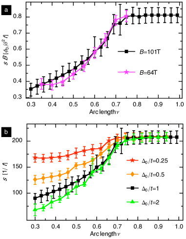
Figure 5: Oscillation frequency in the lattice model. The frequency $s$ is extracted from the power spectrum analysis of oscillations in the low-energy quasiparticle DOS as a function of the arc length $\nu$ with a fixed chemical potential. Panel (a) shows scaling with magnetic field, obtained by considering $16\times 16$ and $20\times 20$ magnetic unit cell. Panel (b) shows the dependence on the gap amplitude at constant field $B$.

VI.4 Action considerations

The quantum oscillations described in Sec. II do not originate from and are not affected by the action quantization. Nevertheless, the action plays an important role in the limit of small gap or large arcs, when Andreev bound states are rare. We use the circular momentum-space trajectory and the Floquet state pseudospin to determine the real-space paths and to calculate the associated action. At energies close to $\epsilon_{F}$ the action is proportional to the energy. To a good approximation $S/\hbar\propto l_{B}^{2}{\cal A}_{k}|\cos(\Delta_{0}\theta_{g}/\hbar\omega_{c})|$ with the magnetic length $l_{B}$ and ${\cal A}_{k}$ the area in $k$-space bounded by the trajectory. Thus, the linear dependence of the action on $1/B$ is modulated by $|\cos(\Delta_{0}\theta_{g}/\hbar\omega_{c})|$, the projection of the pseudospin on the $z$-direction while on the arc. Therefore, for magnetic fields with peaked DOS the action is zero. This means that the Andreev states are allowed by the action quantization. The action slope close to these points is very large (about 3.5 larger than the slope associated with the full Fermi surface area) so that many other states at near magnetic fields are allowed by the action quantization. The fact that more states are allowed does not change the DOS periodicity in $1/B$, however it may broaden the observed oscillation frequency range. When the gapped region shrinks (arc length increases) or the gap amplitude decreases the frequency of DOS modulations due to the Andreev states will decrease. The action quantization then becomes more important. A second frequency which reflects the full Fermi surface area will appear and eventually dominate when the gap closes (the cosine is simply 1 in this limit). In this way our model recovers the usual Onsager-Lifshitz quantization in the limit of vanishing gap.

VI.5 Frequency analysis

We have analyzed the behavior of the oscillation frequency $s$ in the lattice model of Sec. III as a function of magnetic field $B$, arc length $\nu$ and maximum gap size $\Delta_{0}$ (at a fixed chemical potential). Our results are summarized in Fig. 5. The oscillation frequency scales linearly with $1/B$ as expected on the basis of semiclassical Eq. (9). For small and intermediate arc length $\nu$ it increases linearly with $\nu$, also in accord with Eq. (9). Panel (b) shows that the frequency also exhibits dependence of the gap amplitude, not expected on the basis of Eq. (9). This dependence, however, is seen to saturate in the limit of large $\Delta_{0}$. This is consistent with the fact that Eq. (9) is valid only in the regime $\epsilon\ll\Delta_{0}$ and this condition is not fully met in the lattice model for small $\Delta_{0}/t$ since we must consider a finite energy window to extract the oscillation frequency. A more careful analysis of Eq. 16 indeed yields a weak gap dependence of the oscillation frequency $F_{\epsilon}$ with a trend resembling that displayed in Fig. 5b.

References

- (1) J. Bardeen, L.N. Cooper, and J.R. Schrieffer, Phys. Rev. B108, 1175 (1957).
- (2) N. Doiron-Leyraud et al., Nature 447, 565 (2007).
- (3) A. F. Bangura et al., Phys. Rev. Lett. 100, 047004 (2008).
- (4) C. Jaudet et al., Phys. Rev. Lett. 100, 187005 (2008).
- (5) H. Ding et al. Phys. Rev. Lett. 78, 2628 (1997).
- (6) A. Kanigel et al., Nature Phys. 2 447 (2006).
- (7) W.S. Lee et al., Nature 450, 81 (2007).
- (8) L. Onsager, Phil. Mag. 43, 1006 (1952).
- (9) I.M. Lifshitz and A.M. Kosevich, Dokl. Akad. Nauk SSR 96 963 (1954).
- (10) D. Shoenberg, Magnetic oscillations in metals, (Cambridge Univ. Press, 1984).
- (11) A. J. Millis, and M. Norman, Phys. Rev. B 76, 220503(R) (2007).
- (12) S. Chakravarty and H.-Y. Kee, Proc. Natl. Acad. Sci. USA 105, 8835 (2008).
- (13) W.-Q. Chen, K.-Y. Yang, T. M. Rice, and F. C. Zhang, Europhys. Lett. 82, 17004 (2008).
- (14) V. Galitski and S. Sachdev Phys. Rev. B79, 134512 (2009).
- (15) D. Podolsky and H-Y. Kee Phys. Rev. B78, 224516 (2008).
- (16) T. D. Stanescu, V. Galitski, H.D. Drew, Phys. Rev. Lett. 101, 066405 (2008).
- (17) A. Kanigel, U. Chatterjee, M. Randeria, M.R. Norman, G. Koren, K. Kadowaki, and J.C. Campuzano, Phys. Rev. Lett. 101, 137002 (2008).
- (18) A. F. Andreev, Zh. Eksp. Teor. Fiz. 46, 1823 (1964) [Sov. Phys. JETP 19, 1228 (1964)]; I. Adagideli et al. Phys. Rev. Lett. 83, 5571 (1999).
- (19) C. M. Varma Phys. Rev. B79, 085110 (2009).
- (20) A. Melikyan and O. Vafek, Phys. Rev. B78, 020502(R) (2008).
- (21) M.R. Norman, M. Randeria, H. Ding and J.C. Campuzano, Phys. Rev. B52, 615 (1995).
- (22) M. Franz and A.J. Millis, Phys. Rev. B58, 14572 (1998).
- (23) E.Berg and E. Altman, Phys. Rev. Lett. 99, 247001 (2007).
- (24) R.K. Kaul, Y.-B. Kim, S. Sachdev, and T. Senthil, Nature Phys. 4, 28 (2008).
- (25) Y.J. Uemura et al., Phys. Rev. Lett 62, 2317 (1989).
- (26) V. Pasler et al., Phys. Rev. Lett. 81, 1094 (1998).
- (27) J. Corson et al., Nature 398, 221 (1999).
- (28) Z.A. Xu et al., Nature 406, 486 (2000).
- (29) Y. Wang et al., Phys. Rev. Lett. 95, 247002 (2005).
- (30) I. Hetel, T.R Lemberger and M. Randeria, Nature Phys. 3, 700 (2007).
- (31) H. J. Stöckmann Quantum Chaos: an introduction (Cambridge University Press, 1999).
- (32) M.A. Hossain, et al. Nature Phys. 4, 527 (2008).
- (33) M. Franz and Z. Tesanovic, Phys. Rev. Lett. 84, 554 (2000).
- (34) O. Vafek, A. Melikyan, M. Franz and Z. Tešanović, Phys. Rev. B63, 134509 (2001).
- (35) K. Yasui and T. Kita, Phys. Rev. Lett. 83, 4168 (1999).
- (36) L. Marinelli, B. I. Halperin and S. H. Simon, Phys. Rev. B62, 3448 (2000).
- (37) J. Hoffman, K. McElroy, D.-H. Lee, K.M. Lang, H. Eisaki, S. Uchida, and J.C. Davis, Science 297, 1148 (2002).
- (38) K. McElroy, R.W. Simmonds, J.E. Hoffman, D.-H. Lee, J. Orenstein, H. Eisaki, S. Uchida, and J.C. Davis, Nature 422, 592 (2003).
- (39) T. Pereg-Barnea and M. Franz, Phys. Rev. B78, 020509 (2008).