COLLECTIVE FLAVOUR TRANSITIONS OF SUPERNOVA NEUTRINOS

When the neutrino density is very high, as in core-collapse supernovae, neutrino-neutrino interactions are not negligible and can appreciably affect the evolution of flavour. The physics of these phenomena is briefly highlighted, and their effects are shown on observable energy spectra from a future galactic supernova within $2\nu$ and $3\nu$ frameworks. Detection of such effects could provide a handle on two unknowns: the neutrino mass hierarchy, and the mixing angle $\theta_{13}$.

1 Introduction

Neutrino flavour eigenstates ($\nu_{e}$, $\nu_{\mu}$, $\nu_{\tau}$) are related to mass eigenstates ($\nu_{1}$, $\nu_{2}$, $\nu_{3}$) by means of an unitary matrix $U$, espressed in terms of three mixing angles $\theta_{ij}$ and one phase $\delta$ associated to possible CP violation.

We know rather precisely two squared mass differences ($\delta m^{2}$ and $\Delta m^{2}$, with $\delta m^{2}\ll\Delta m^{2}$) and two mixing angles ($\theta_{12}$ and $\theta_{23}$). However we do not know yet the sign of $\Delta m^{2}$ (i.e., if the mass hierarchy is normal or inverted), nor the value of $\theta_{13}$ or of $\delta$. Some hints about the mass hierarchy and the mixing angle $\theta_{13}$ could come from future core-collapse supernova events in our galaxy (estimated to occur at a rate of a few per century).

In ordinary matter, neutrinos of all flavours are subject to neutral current interactions, whereas $\nu_{e}$’s are also subject to charged current interactions on electrons. The $\nu_{e}-\nu_{\mu,\tau}$ interaction energy difference is described by the Mikheev-Smirnov-Wolfestein (MSW) matter potential

$$\lambda(r)=\sqrt{2}\,G_{F}\,N_{e}(r)\ ,$$ (1)

where $N_{e}(r)$ is the electron number density; see $\!{}^{{\bf?}}$ for a review.

When the neutrino density is very high, as in core-collapse supernovae, $\nu-\nu$ forward scattering may also become important  $\!{}^{{\bf?}}$. Such interactions induce large, non-linear and collective flavour conversions. Since neutrinos of different flavours are coupled during their evolution history, collective effects are very different from neutrino oscillations in matter, and they are described by means of the self-interaction potential $\mu$. For this purpose, for each species $\nu_{\alpha}$, it is useful to introduce the effective density $n_{\alpha}$ per unit of volume and of energy $\!{}^{{\bf?}}$. After energy integration, we get the total effective density of $\nu$ ($N=N_{e}+N_{\mu}+N_{\tau}$) and of $\bar{\nu}$ ($\overline{N}=\overline{N}_{e}+\overline{N}_{\mu}+\overline{N}_{\tau}$) per unit volume. The potential $\mu$, at any radius $r$, reads

$$\mu(r)=\sqrt{2}\,G_{F}\,[N(r)+\overline{N}(r)]\ .$$ (2)

Figure 1 $\!{}^{{\bf?}}$ shows the matter and self-interaction potentials ($\lambda$ and $\mu$), at a representative time $t=5$ s after the core-bounce, for a supernova spherically-symmetric bulb model $\!{}^{{\bf?}}$ with a neutrinosphere radius $R_{\nu}=10$ km.

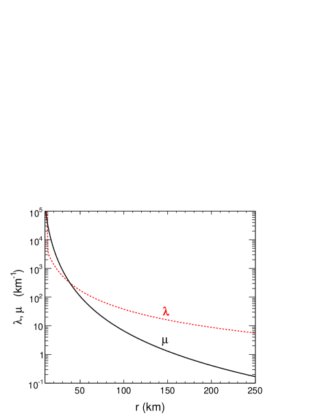
Figure 1: Radial profiles adopted for the matter ($\lambda$) and self-interaction ($\mu$) potentials, in the range $r\in[10,\,250]$ km, at $t=5$ s after the core-bounce.

The typical range for the vacuum oscillation frequency $\omega_{H}=\Delta m^{2}/2E$ is $\omega_{H}\in[0.1,5.1]$ km^-1 for $\Delta m^{2}=2\times 10^{-3}$ eV². Therefore, at small radii ($r\in[10,200]$ km) self-interactions are not negligible ($\mu\sim\omega$). Usual MSW effects take place later (when $\lambda\sim\omega$) and, finally, vacuum mixing must also be considered.

In our reference supernova scenario $\!{}^{{\bf?}}$, we assume a galactic core-collapse supernova releasing a binding energy $E_{B}=3\times 10^{53}$ erg, equally distributed among the six neutrino and antineutrino species, with luminosity decreasing with a time constant $\tau=3$ s. The unoscillated flux of the neutrino species $\nu_{\alpha}$, per unit of area, time and energy, is then

$$F^{0}_{\alpha}(E,\,t)=\frac{e^{-t/\tau}}{\tau}\frac{E_{B}}{24\pi R_{\nu}^{2}}\,\frac{\phi^{0}_{\alpha}(E)}{\langle E_{\alpha}\rangle}\ ,$$ (3)

where we assume normalized thermal energy spectra $\phi^{0}_{\alpha}(E)$ $\!{}^{{\bf?},{\bf?},{\bf?}}$ with average energy $\langle E_{\alpha}\rangle$. The numerical values used for the mean energies are $\langle E_{e}\rangle=10$ MeV, $\langle E_{\mu,\tau}\rangle=\langle\overline{E}_{\mu,\tau}\rangle=24$ MeV, $\langle\overline{E}_{e}\rangle=15$ MeV, where the bar labels antineutrinos.

2 Collective effects in a two-flavour scenario

In a core-collapse supernova, because of the typical neutrino energies [$E\sim O(10)$ MeV], $\nu_{\mu}$ and $\nu_{\tau}$ are both below the threshold for $\mu$ and $\tau$ production and have the same interactions. In a two-flavour approximation, we can neglect the small mass difference $\delta m^{2}$ and consider an effective two-family $(\nu_{e},\nu_{x})$ scenario where $\nu_{x}$ is either $\nu_{\mu}$ or $\nu_{\tau}$, and there are only two mass-mixing parameters, $\Delta m^{2}=2\times 10^{-3}$ eV² and $\sin^{2}\theta_{13}<$ few $\%$. We set $\sin^{2}\theta_{13}=10^{-4}$, but the precise value is not very important in this context.

In the flavour basis, the neutrino system is described by a $2\times 2$ density matrix for each energy mode. Decomposing the density matrix over the Pauli matrices, the evolution of the system can be explained in terms of the Bloch vectors $\mathbf{P}$ and $\overline{\mathbf{P}}$ ($|\mathbf{P}|=|\overline{\mathbf{P}}|=1$) , for $\nu$ and $\bar{\nu}$ respectively. After trajectory averaging (single-angle approximation $\!{}^{{\bf?}}$), the $\mathbf{P}$ and $\overline{\mathbf{P}}$ modes obey equations of motion which resemble precessions,

$$\dot{\mathbf{P}} = \left(+\omega_{H}\mathbf{B}+\lambda\mathbf{z}+\frac{\mu}{N+\overline{N}}\,{\int_{0}^{\infty}dE\,(n\,\mathbf{P}-\overline{n}\;\overline{\mathbf{P}})}\right)\times\mathbf{P}\ ,$$ (4)

$$\dot{\overline{\mathbf{P}}} = \left(-\omega_{H}\mathbf{B}+\lambda\mathbf{z}+\frac{\mu}{N+\overline{N}}\,{\int_{0}^{\infty}dE\,(n\,\mathbf{P}-\overline{n}\;\overline{\mathbf{P}})}\right)\times\overline{\mathbf{P}}\ ,$$ (5)

where $\mathbf{B}$ is a three-dimensional “magnetic field” vector embedding $\theta_{13}$ $\!{}^{{\bf?},{\bf?}}$. For each energy mode, the third component of $\mathbf{P}$ ($P_{z}$) is related to the survival probability at the time $t$:

$$P_{\nu_{e}\rightarrow\nu_{e}}(t)=\frac{1}{2}\left(1+\frac{P_{z}(t)}{P_{z}(0)}\right)\ .$$ (6)

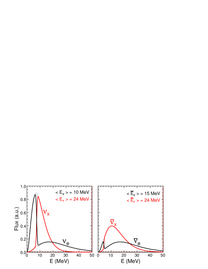
Figure 2: Single-angle simulation in inverted hierarchy: Fluxes at the end of collective effects (at $r=250$ km, in arbitrary units) for different neutrino species, as a function of energy. Initial fluxes ($r=10$ km) are shown as dotted lines to guide the eye, with average energies reported on top.

Figure 2 $\!{}^{{\bf?}}$ shows the fluxes $F_{\alpha}^{\prime}$ at the end of collective effects ($r\sim$ few $\times\ 100$ km) with respect to the unoscillated ones $F_{\alpha}^{0}$. In inverted hierarchy, a full flavour swap takes place at certain energies ($E_{c}\sim 7$ MeV for $\nu$ and $\overline{E}_{c}\sim 4$ MeV for $\bar{\nu}$, in our scenario) $\!{}^{{\bf?},{\bf?},{\bf?}}$. This full flavour conversion is called spectral split and is an important signature of collective effects $\!{}^{{\bf?},{\bf?},{\bf?},{\bf?}}$. It takes place only in inverted hierarchy, for any $\theta_{13}\neq 0$ $\!{}^{{\bf?}}$. If the hierarchy is normal or if $\theta_{13}\equiv 0$, then $F_{\alpha}^{\prime}\simeq F_{\alpha}^{0}$ for each $\nu_{\alpha}$ (i.e., there are no significant conversion effects).

3 Self-interactions in a three-flavour scenario

The two-flavour approximation captures several features of collective effects. Are these effects unchanged in a three-flavour analysis? For this purpose, we have developed a framework with three neutrino families $\!{}^{{\bf?}}$, using all three mixing angles ($\sin^{2}\theta_{13}=10^{-6}$, $\sin^{2}\theta_{12}=0.314$, $\sin^{2}\theta_{23}\in[0.5,0.36,0.64]$), both mass differences ($\delta m^{2}=8\times 10^{-5}$ eV² and $\Delta m^{2}=2\times 10^{-3}$ eV²) and including the one-loop $\nu_{\mu}-\nu_{\tau}$ matter potential correction $\!{}^{{\bf?}}$. We consider the evolution at four different times ($t=1,5,10,20$ s) after the core-bounce.

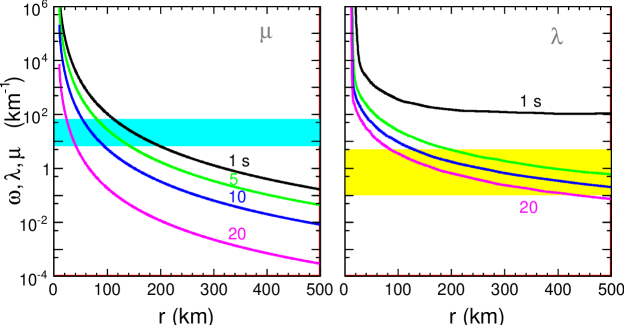
Figure 3: Radial profiles of the self-interaction potential $\mu$ (left) and of the matter potential $\lambda$ (right). The black, green, blue and magenta curves correspond to $t=1$, 5, 10, and 20 s, respectively. In the left panel, the shaded horizontal band marks the $\mu$ range where bipolar effects develop. In the right panel, the shaded band marks the range of $\omega_{H}$ for $E\in[1,\,50]$ MeV, where MSW effects may develop, if the $H$-resonance condition ($\lambda\sim\omega_{H}$) is satisfied and if $\sin^{2}\theta_{13}>10^{-5}$.

The self-interaction and matter potentials are plotted in Fig. 3. We expect that collective effects take place at different radii for different $t$, and MSW effects take place after collective ones. In this particular case, MSW oscillations are not relevant because of the tiny value of $\theta_{13}$ chosen. According to this choice, after collective effects, we have only to consider $\theta_{12}$ mixing to get the final $\nu$ fluxes to the Earth.

In three generations, the density operator is a $3\times 3$ matrix in flavour basis. Decomposition over Gell-Mann matrices provides eigth-dimensional Bloch vectors ($|\mathbf{P}|=|\overline{\mathbf{P}}|=2/\sqrt{3}$). For each energy mode, the evolution equations in inverted hierarchy are

$$\dot{\mathbf{P}} = \left[+(\omega_{L}\mathbf{B}_{L}-\omega_{H}\mathbf{B}_{H})+\lambda\mathbf{v}+\frac{\mu}{N+\overline{N}}\,{\int_{0}^{\infty}dE\,(n\,\mathbf{P}-\overline{n}\;\overline{\mathbf{P}})}\right]\times\mathbf{P}\ ,$$ (7)

$$\dot{\overline{\mathbf{P}}} = \left[-(\omega_{L}\mathbf{B}_{L}-\omega_{H}\mathbf{B}_{H})+\lambda\mathbf{v}+\frac{\mu}{N+\overline{N}}\,{\int_{0}^{\infty}dE\,(n\,\mathbf{P}-\overline{n}\;\overline{\mathbf{P}})}\right]\times\overline{\mathbf{P}}\ .$$ (8)

In the above equations, the first (vacuum) terms embed the squared mass splittings via $\omega_{L,H}$ (with $\omega_{L}=\delta m^{2}/2E$), and the mixing angles via two “magnetic fields”, $\mathbf{B}_{L,H}$ $\!{}^{{\bf?}}$. The second (matter interaction) term, $\lambda\mathbf{v}$, also includes the $\nu_{\tau}-\nu_{\mu}$ potential difference at one loop $\!{}^{{\bf?},{\bf?},{\bf?}}$, whose size is $\delta\lambda/\lambda\simeq 5\times 10^{-5}$; the vector $\mathbf{v}$ is a linear combination of the unitary vectors $\mathbf{u}_{3}$ and $\mathbf{u}_{8}$.

In the three-flavour scenario, the survival probability is a linear combination of the third and the eighth components $\!{}^{{\bf?}}$. In fact the analogous of the third component of $\mathbf{P}$ in the two-flavour approximation is, in the three-flavour case, a linear combination of the third and eighth ones:

$$P_{z}\rightarrow P_{3}+\frac{P_{8}}{\sqrt{3}}\ .$$ (9)

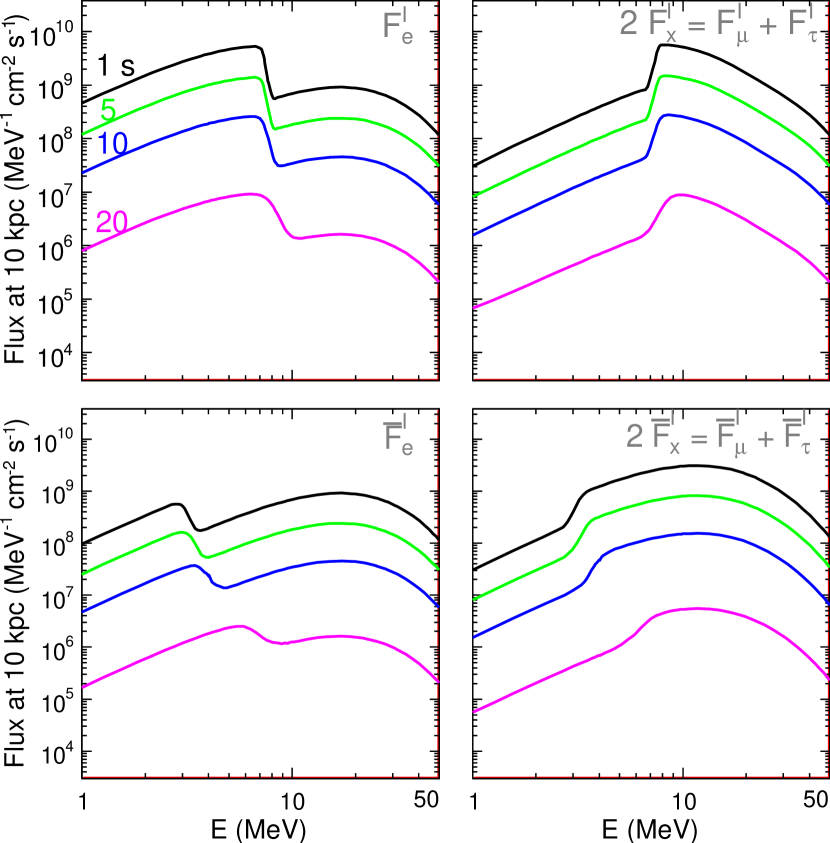
Figure 4: Single-angle simulation in inverted hierarchy: Fluxes of $\nu$ ($F^{\prime}_{\alpha}$) and $\bar{\nu}$ ($\overline{F}^{\prime}_{\alpha}$) for four different $t$ after the core-bounce and at the end of collective effects, rescaled to $d=10$ kpc.

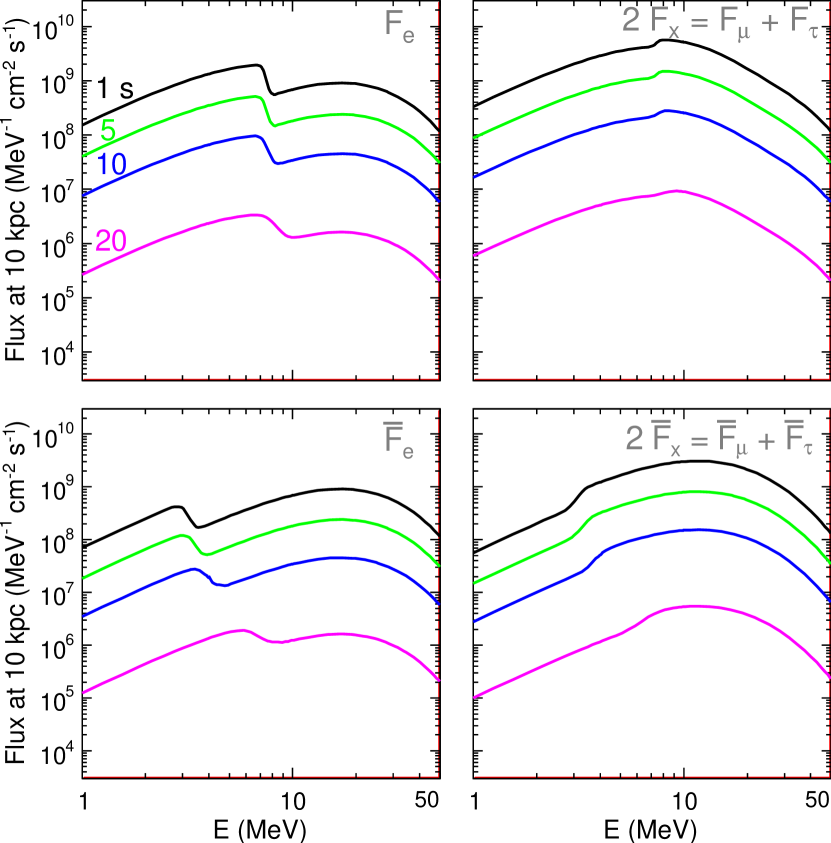
Figure 5: Single-angle simulation in inverted hierarchy: Final oscillated fluxes of $\nu$ ($F_{\alpha}$) and $\bar{\nu}$ ($\overline{F}_{\alpha}$) at $d=10$ kpc (collective effects + vacuum propagation).

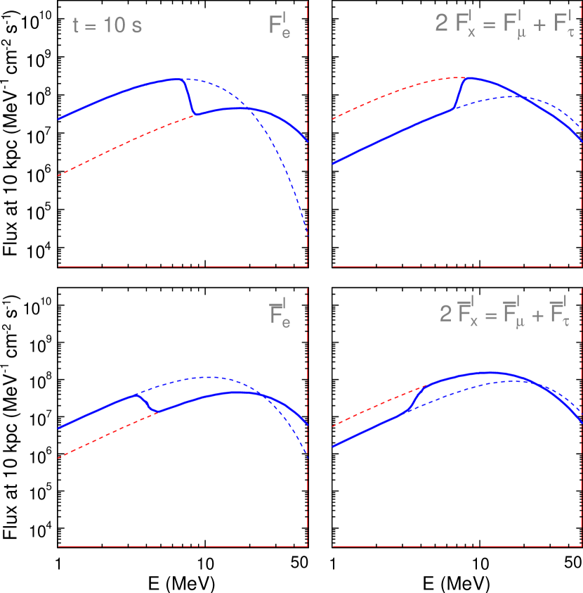
Figure 6: Single-angle simulation in inverted hierarchy: Fluxes of $\nu$ and $\bar{\nu}$ at the end of collective effects, for $t=10$ s. Solid curves: computed fluxes $F_{\alpha}^{\prime}$. Dashed blue and red curves: limiting behavior at low and high energies, respectively, in terms of unoscillated fluxes $F_{\alpha}^{0}$, according to Eqs. 10.

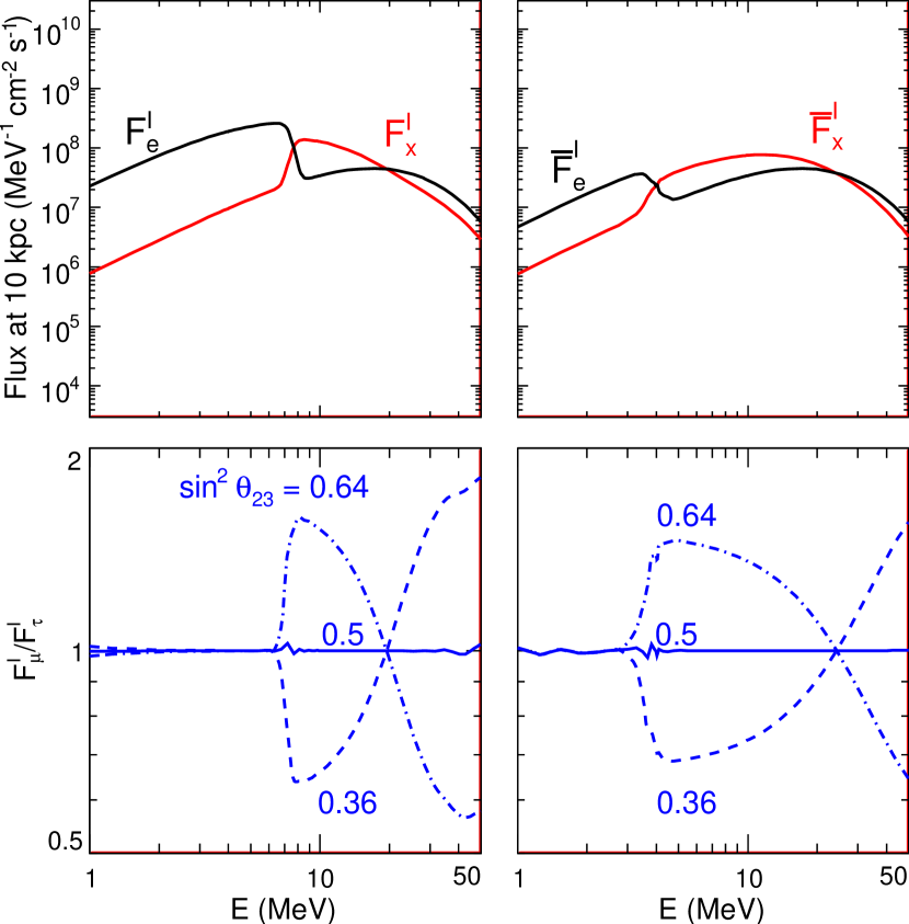
Figure 7: Single-angle simulation in inverted hierarchy: Neutrino and antineutrino fluxes $F^{\prime}_{\alpha}$ at the end of collective effects ($r<500$ km), for $t=10$ s. Upper panels: absolute fluxes. Lower panels: muonic-to-tauonic flux ratio for $\nu$ (left) and $\overline{\nu}$ (right), for $\sin^{2}\theta_{23}=0.36,\,0.5,\,0.64$.

Figure 5 shows the intermediate fluxes, $F^{\prime}_{\alpha}(E,t)$, at the end of collective effects ($r\simeq 500$ km) for four different times after the core-bounce. Figure 5 shows the corresponding fluxes $F_{\alpha}(E,\,t)$ at the Earth i.e., including final vacuum mixing effects. Split signatures of collective effects are still visible in $\nu_{e}$ and $\bar{\nu}_{e}$ fluxes of Fig. 5, and they are similar for different times after the core-bounce. In view of prospective observations of galactic supernova neutrino bursts, the persistence of similar stepwise features for several seconds is useful, because we may expect to see them also in time-integrated spectra. The $x$-flavour split features in Fig. 5 are suppressed by $\theta_{12}$ mixing with respect to Fig. 5.

In a two-flavour analysis a full flavour conversion ($\nu_{e},\nu_{x}$) takes place above certain energies ($E>E_{c}$ for $\nu$ and $E>\overline{E}_{c}$ for $\bar{\nu}$), while in the three-flavour framework one linear combination of $\nu_{\mu}$ and $\nu_{\tau}$ remains a “spectator”, so that:

$$F^{\prime}_{e}\simeq\left\{\begin{array}[]{ll}F^{0}_{e}&(E<E_{c})\\ F^{0}_{x}&(E>E_{c})\end{array}\right.~{}~{}~{}~{}~{}~{}~{}~{}~{}~{}~{}\mathrm{and}~{}~{}~{}~{}~{}~{}~{}~{}~{}~{}~{}~{}~{}~{}2F^{\prime}_{x}\simeq\left\{\begin{array}[]{ll}2F^{0}_{x}&(E<E_{c})\\ F^{0}_{e}+F^{0}_{x}&(E>E_{c})\end{array}\right.$$ (10)

and similarly is for antineutrinos. This limiting behavior is shown in Fig. 7: the solid curves (oscillated fluxes) exactly superimpose to the dashed ones (linear combinations of non-oscillated fluxes, as in Eqs. 10).

Supernova neutrino fluxes are, in principle, sensitive to the specific value of $\theta_{23}$. In fact if $\theta_{23}$ belongs to the first (second) octant, a leading $\nu_{e}\rightarrow\nu_{\tau}$ ($\nu_{e}\rightarrow\nu_{\mu}$) takes place, or if $\theta_{23}$ is maximal, $\nu_{\mu}$ and $\nu_{\tau}$ fluxes are exactly equal  $\!{}^{{\bf?}}$. This different behaviour in $\nu_{e}$ conversion (in $\nu_{\mu}$ or in $\nu_{\tau}$) according to the specific value of the mixing angle $\theta_{23}$ is shown in Fig. 7. Unfortunately, $\nu_{\mu}$ and $\nu_{\tau}$ fluxes cannot be separately detected.

Although collective split signatures are similar in two and three-flavour scenarios, it is worth stressing that the former is not a limit of the latter, because the $\nu-\nu$ interaction physics depends on the absolute luminosities (which are different, if shared among two or three flavours).

4 Conclusions

Neutrino-neutrino interactions are not negligible when the neutrino density is very high, as in core-collapse supernovae. $\nu-\nu$ interactions are sensitive to the mass hierarchy and $\theta_{13}$. In fact, if the hierarchy is inverted and $\theta_{13}\neq 0$, split features are observable in the spectra. Otherwise if $\theta_{13}=0$ or the hierarchy is normal, there are no significant conversion effects in general.

A two-flavour approximation is useful to analyze the qualitative behavior; however the total neutrino luminosity influences the evolution, and it changes if it is distributed on two or three families. As a consequence, three-generation analyses are important to validate the results.

References

References

- [1] T. K. Kuo, J. Pantaleone, Rev. Mod. Phys. 61, 937 (1989).
- [2] J. T. Pantaleone, Phys. Lett. B 287, 128 (1992).
- [3] H. Duan, G. M. Fuller, J. Carlson and Y. Z. Qian, Phys. Rev. D 74, 105014 (2006).
- [4] G. L. Fogli, E. Lisi, A. Marrone, A. Mirizzi and I. Tamborra, Phys. Rev. D 78, 097301 (2008).
- [5] R. C. Schirato and G. M. Fuller, arXiv:astro-ph/0205390.
- [6] G.L. Fogli, E. Lisi, A. Marrone, and A. Mirizzi, JCAP 12, 010 (2007).
- [7] G. L. Fogli, E. Lisi, A. Marrone, I. Tamborra, JCAP 0904, 030 (2009).
- [8] H. Duan, G. M. Fuller and Y. Z. Qian, Phys. Rev. D 76, 085013 (2007).
- [9] G.G. Raffelt and A.Y. Smirnov, Phys. Rev. D 76, 125008 (2007).
- [10] H. Duan, G.M. Fuller and Y.Z. Qian, Phys. Rev. D 74, 123004 (2006).
- [11] G.G. Raffelt and A.Y. Smirnov, Phys. Rev. D 76, 081301 (2007) [Err. 77, 029903 (2008)].
- [12] H. Duan, G.M. Fuller, J. Carlson and Y.-Z. Quian, Phys. Rev. Lett. 99, 241802 (2007).
- [13] A. Esteban-Pretel, S. Pastor, R. Tomas, G.G. Raffelt and G. Sigl, Phys. Rev. D 76, 125018 (2007).
- [14] S. Hannestad, G.G. Raffelt, G. Sigl and Y.Y.Y. Wong, Phys. Rev. D 74, 105010 (2006) [Err. 76, 029901 (2007)].
- [15] F.J. Botella, C.S. Lim and W.J. Marciano, Phys. Rev. D 35, 896 (1987).
- [16] A. Esteban-Pretel, S. Pastor, R. Tomas, G. G. Raffelt and G. Sigl, Phys. Rev. D 77, 065024 (2008).
- [17] H. Duan, G. M. Fuller and Y. Z. Qian, Phys. Rev. D 77, 085016 (2008).
- [18] B. Dasgupta and A. Dighe, Phys. Rev. D 77, 113002 (2008).