Tsallis statistics as a tool for studying interstellar turbulence

Abstract

We used magnetohydrodynamic (MHD) simulations of interstellar turbulence to study the probability distribution functions (PDFs) of increments of density, velocity, and magnetic field. We found that the PDFs are well described by a Tsallis distribution, following the same general trends found in solar wind and Electron MHD studies. We found that the PDFs of density are very different in subsonic and supersonic turbulence. In order to extend this work to ISM observations we studied maps of column density obtained from 3D MHD simulations. From the column density maps we found the parameters that fit to Tsallis distributions and demonstrated that these parameters vary with the sonic and Alfvén Mach numbers of turbulence. This opens avenues for using Tsallis distributions to study the dynamical and perhaps magnetic states of interstellar gas.

1. Introduction

Turbulence is known to be a crucial ingredient in many astrophysical phenomena that take place in the interstellar medium (ISM): such as star formation, cosmic ray dispersion, formation and evolution of the (also very important) magnetic field, and virtually every transport process (see for instance the reviews of Elmegreen & Scalo 2004; Mac Low & Klessen 2004; Ballesteros-Paredes et al. 2007; McKee & Ostriker 2007, and references therein). This has brought many researchers to the study of turbulence, from both observational and theoretical perspectives.

From the observational point of view there are several techniques aimed to study properties of ISM turbulence. Scintillation studies (see for instance Narayan & Goodman, 1989; Spangler & Gwinn, 1990) have been very successful to characterize ISM turbulence, however they are limited to density fluctuations in only ionized media. For neutral media the density fluctuations can also be obtained from column density maps (see Padoan et al., 2003). Other avenue of research is provided by radio spectroscopic observations, using for instance the centroids of spectral lines (von Hoerner, 1951; Münch, 1958; Dickman & Kleiner, 1985; Kleiner & Dickman, 1985; O’Dell & Castaneda, 1987; Falgarone et al., 1994; Miesch & Bally, 1994; Miesch & Scalo, 1995; Lis et al., 1998; Miesch et al., 1999), or linewidth maps (Larson, 1981, 1992; Scalo, 1984, 1987). Spectroscopic observations have the advantage of containing information about the underlying turbulent velocity field. However, they are also sensitive to fluctuations in density, and the separation of the two contributions alone has proved to be a difficult problem (see Lazarian, 2006b).

Much of the effort to relate observations with models of turbulence has focused on obtaining the spectral index (log-log slope of the power-spectrum) of density and/or velocity. To this purpose several methods have been developed and tested through numerical simulations. Among them, we can mention the “Velocity Channel Analysis” (VCA, Lazarian & Pogosyan, 2000; Esquivel et al., 2003; Lazarian & Pogosyan, 2004; Lazarian et al., 2001; Padoan et al., 2003; Chepurnov & Lazarian, 2009), the “Spectral Correlation Function” (SCF Rosolowsky et al., 1999; Padoan et al., 2001), “Velocity coordinate spectrum” (Lazarian & Pogosyan, 2008, 2006), or “Modified Velocity Centroids” (Lazarian & Esquivel, 2003; Esquivel & Lazarian, 2005; Ossenkopf et al., 2006; Esquivel et al., 2007; Chepurnov et al., 2006; Chepurnov & Lazarian, 2009; Padoan et al., 2009) Different methods are suitable in different situations, for instance VCA is adequate to retrieve velocity information from supersonic turbulence, while centroids are only useful in subsonic (or at most, transonic) turbulence.

More sophisticated techniques for the analysis of the data, including using wavelets instead of Fourier transforms (Henriksen, 1994; Stutzki et al., 1998) have been attempted. A rather sophisticated example of such analysis is a use of the Principal Component Analysis(PCA) (Heyer & Schloerb, 1997; Brunt & Heyer, 2002).

The techniques above provide the spectrum of turbulent velocity and/or density. Spectra, however, do not provide a complete description of turbulence. For example, Chepurnov et al. (2008) showed that fields with a very different distribution of density could have the same power spectrum. Intermittency and topology are some of the turbulence features that require additional statistical tools. Measures of turbulence intermittency include probability distribution functions (PDFs, see for instance Falgarone et al. 1994; Lis et al. 1996, 1998; Klessen 2000), higher-order She-Lévêque exponents (She & Lévêque, 1994; Padoan et al., 2003; Falgarone et al., 2005; Hily-Blant et al., 2008). In addition, genus (see also Lazarian et al., 2002; Kim & Park, 2007; Chepurnov et al., 2008) was used to study the topological structure of the diffuse gas distribution.

Astrophysical turbulence is very complex, e.g. it can happen in the multi-phase media with numerous energy sources. Therefore the synergy of different techniques provide an invaluable insight into the properties of the ISM turbulence and the self-organization of interstellar medium. For instance, Kowal et al. (2007) and Burkhart et al. (2009) have applied several statistical measures, including a measure of bispectrum, to a wide set of MHD simulations and synthetic-observational data. More recent work applying the same set of techniques to the Small Magellanic Cloud (SMC) data revealed the advantages of such an approach (Burkhart et al., 2010). It is the consistency of the results obtained by different techniques, which made the study of turbulence properties in SMC more reliable.

Thus it is important to proceed with the quest for new techniques for astrophysical studies (see Lazarian 2009 and ref. therein). In this paper we add the Tsallis statistics to the arsenal of tools available for ISM studies of turbulence. This is a description of the PDFs that have been successfully used previously in the context of solar wind observations and it shares similarities to previous studies of ISM turbulence (e.g. Klessen, 2000).

The earlier solar wind relation between the Tsallis statistics and turbulence was sought on the basis of 1D MHD simulations. We know that the properties of turbulence strongly depend on its dimensions. Thus we use 3D MHD simulations. We analyze a reduced set of MHD simulations, including column density maps which are the most easily available data from observations.

This paper is organized as follows. In section 2 we briefly present the Tsallis distribution, which we will use to characterize magnetohydrodynamic (MHD) simulations. The description of the numerical models and the results (for 3D data as well as column density) can be found in sections 3–5. We discuss the significance of our findings in 6. Finally, in section 7 we provide our summary.

2. Tsallis Statistics

Burlaga & Viñas (2004a, b, 2005a, 2005b); Burlaga, Ness, & Acuña (2006a, b); Burlaga & Viñas (2006); Burlaga, Viñas, & Wang (2007b, a, 2009), have studied the PDFs of the variation of the magnetic field strength in the solar wind, measured by the Voyager 1 and 2 spacecrafts. In particular, they analyzed the fluctuations of magnetic field increments $[B(t+\tau_{m})-B(t)]$ as a function of the timescale $\tau_{m}$, and showed that for a wide range of scales their PDFs could be described by a Tsallis (or $q$-Gaussian) distribution (Tsallis, 1988). The Tsallis PDF of increments ($\Delta f$) of an arbitrary function has the form:

$$R_{q}=A\left[1+\left(q-1\right)\frac{\Delta f\left(t,\tau\right)^{2}}{w^{2}}\right]^{-1/(q-1)},$$ (1)

where $q$ is the so called “entropic index” or “non-extensivity parameter” and is related to the size of the tail of the distribution, $w$ provides a measure of the with of the PDF (related to the dispersion of the distribution), while $A$ measures the amplitude. Notice that the Tsallis distribution is symmetric. Varying the parameter $q$ in the Tsallis distribution one obtain distributions that range from Gaussian to “peaky” distributions with large tails. The parameter $q$ is closely related to the kurtosis (fourth order one-point moment) of the PDF, and similarly the parameter $w$ is related to the variance of the PDF. However, they are not the same, while fitting a Tsallis distribution to a PDF, the two parameters are calculated simultaneously, therefore $w$ will depend on the value of $q$ and vice versa, while the dispersion of a distribution is independent of the kurtosis. In the next section we discuss how this difference might play in our favor. Furthermore, the Tsallis distribution is often used in the context of non-extensive statistical dynamics, it was originally derived (Tsallis, 1988) from an entropy generalization to extend the traditional Boltzmann-Gibbs statistics to multifractal systems (such as the ISM). The Tsallis distribution reduces to the classical Boltzmann-Gibbs (Gaussian) distribution in the limit of $q\rightarrow 1$. It provides a physical foundation to other functions that have been used to model empirically velocity PDFs in space plasmas (such as the kappa function, see Maksimovic et al., 1997; Leubner, 2002). However, the physical interpretation of ISM simulations/observations PDFs in the light of such statistical dynamics is beyond the scope of this paper.

Turbulence intermittency manifests itself in non-Gaussian distributions, thus one can hope to establish a link between the properties of turbulence and the Tsallis distributions parameters obtained from simulations and/or observations. This provides an alternative/complementary method to higher order statistics (Burkhart et al., 2009), or to other PDF analysis (such as those in Falgarone et al., 1994; Klessen, 2000, where the kurtosis and/or skewness of the distributions is measured), all of which are sensitive to the non-Gaussian nature of real turbulence.

Following the procedure presented by Burlaga and collaborators in what follows we make histograms of the distribution of fluctuations from our simulations. But, in contrast to their studies, where only the magnetic field variations were studied at different times, we consider the spatial variations of density, velocity and magnetic field intensity at a given time, as a function of a spatial scale (or lag) $r$. To make the fits and present the results we remove the mean value of the increments and scale them to units of the standard deviation of each PDF. In other words, we have used $\Delta f(r)=[f(r)-\langle f(r)\rangle_{\mathbf{x}}]/\sigma_{f}$, with $f(\mathbf{x})=\rho(\mathbf{x}+r)-\rho(\mathbf{x})$, $v_{x}(\mathbf{x}+r)-v_{x}(\mathbf{x})$, $v_{y}(\mathbf{x}+r)-v_{y}(\mathbf{x})$, $v_{z}(\mathbf{x}+r)-v_{z}(\mathbf{x})$, $B_{x}(\mathbf{x}+r)-B_{x}(\mathbf{x})$, $B_{y}(\mathbf{x}+r)-B_{y}(\mathbf{x})$, and $B_{z}(\mathbf{x}+r)-B_{z}(\mathbf{x})$, where $\langle...\rangle_{\mathbf{x}}$ stands for spatial average. We have neglected the anisotropy introduced by the magnetic field (see Cho & Lazarian, 2009), the lag $r$ is considered along each of the three cardinal directions and the resulting histograms include variations in all of them.

3. MHD simulations

We have taken a reduced subset of the MHD simulations of fully-developed (driven) turbulence of Kowal et al. (2007). We use the data output of the simulations to study the resulting PDFs of density, magnetic field and velocity in different turbulence scenarios.

The code used (described in detail in Kowal et al. 2007) solves the ideal MHD equations in conservative form:

$$\frac{\partial\rho}{\partial t}+\mathbf{\nabla\cdot}\left(\rho\mathbf{v}\right)=0,$$ (2)

$$\frac{\partial\rho\mathbf{v}}{\partial t}+\mathbf{\nabla\cdot}\left[\rho\mathbf{vv}+\left(p+\frac{B^{2}}{8\pi}\right)\mathbf{I}-\frac{1}{4\pi}\mathbf{BB}\right]=\mathbf{f},$$ (3)

$$\frac{\partial\mathbf{B}}{\partial t}-\mathbb{\nabla\times}\left(\mathbf{v\times B}\right)=\mathbf{0},$$ (4)

along with the additional constraint $\mathbf{\nabla\cdot B}=0$ in a Cartesian, periodic domain. An isothermal equation of state $p=c_{s}^{2}\rho$ is used, where $\rho$ is the mass density, $\mathbf{v}$ the velocity, $\mathbf{B}$ the magnetic field, $p$ the gas pressure, and $c_{s}$ the isothermal sound speed. The term $\mathbf{f}$ in the equation of momentum (3) is a large scale driving. The driving is purely solenoidal, applied in Fourier space at a fixed wave-number $k=2.5$ (a scale $2.5$ times smaller than the size of the computational box). The rms velocity is maintained close to unity, so that $v$ is in units of the rms velocity of the system, the Alfvén velocity $v_{A}=\mathbf{B}/(4\pi\rho)^{1/2}$ is also in the same units. The magnetic field is of the form $\mathbf{B}=\mathbf{B}_{\mathrm{ext}}+\mathbf{b}$, that is a uniform background field $\mathbf{B}_{\mathrm{ext}}$ plus a fluctuating part $\mathbf{b}$ (initially equal to zero). As it is customary, the units are normalized such that the Alfén velocity $v_{A}=B_{\mathrm{ext}}/(4\pi\rho)^{1/2}=1$ and the mean density $\rho_{0}=1$. This way, the controlling parameters are the sound, and the Alfvén speeds (i.e. the gas pressure and the magnetic pressure, respectively), yielding any combination of subsonic or supersonic, with sub-Alfvénic or super-Alfvénic regimes of turbulence. For this paper we explore the different combinations of parameters summarized in Table 1.

Table 1Parameters of the simulations

Model	$p$	$B_{\mathrm{ext}}$	$\mathcal{M}_{s}$	$\mathcal{M}_{A}$	Description
1	0.1	0.1	2.0	2.0	Supersonic & super-Alfvénic
2	0.1	1.0	2.0	0.7	Supersonic & sub-Alfvénic
3	1.0	0.1	0.7	2.0	Subsonic & super-Alfvénic
4	1.0	1.0	0.7	0.7	Subsonic & sub-Alfvénic

We should note that it has been recently found that a compressive component of the driving can have an important effect on the statistical properties of the flow (Schmidt et al., 2008; Federrath et al., 2008; Schmidt et al., 2009). This is an interesting effect that require further study, but for the time being we will restrict ourselves to the usual divergence-free driving.

4. Statistics of three-dimensional data

Below, we analyze the results of our simulations to test whether the statistics of the PDFs of the fluctuations of the variables can be described by the Tsallis formalism. To to this we fit to each histogram a Tsallis distribution with the Levenberg-Marquardt algorithm (Press et al., 1992), the histograms and the fits are presented in Figure 1, the symbols are the data from the simulations, and the lines are the corresponding fits. For visual purposes we have shifted vertically the results by successive factors of $100$ for each different lag.

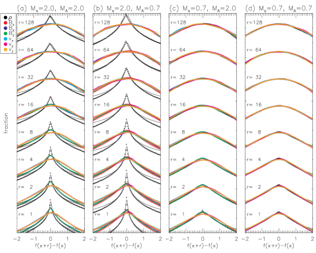
Figure 1.— PDFs of fluctuations for different spatial lags $r$, for all the models. The symbols represent data from the numerical simulations and the lines are the fits with a q-Gaussian (Tsallis) distribution. The different MHD variables are color coded according to the legend at the upper left corner, and the value of the lag is indicated at the left of each set of curves.

Similarly to the results from solar wind observations (Burlaga & Viñas, 2004a, b, 2005a, 2005b; Burlaga et al., 2006a, b; Burlaga & Viñas, 2006; Burlaga et al., 2007a, b, 2009), the magnetic field components, as well as the density and velocity components, show kurtotic PDFs that become smoother as we increase the scale-length (lag). One difference is the fact that the velocity increments in our simulations are symmetric, as opposed to the skewed distributions observed in the solar wind at small scales. It is also interesting that (only) for supersonic turbulence density distributions are quite distinct from other quantities. Such behavior resembles the power spectrum, where the magnetic field and velocity for supersonic turbulence have steep spectra regardless of sonic Mach number, while density becomes shallower as the Mach number increases (see for instance Esquivel & Lazarian, 2005). Such shallower slopes of the density power-spectrum have been also reported when the driving changes from solenoidal to compressive (potential) for a fixed ($>1$) sonic Mach number (Federrath et al., 2009). This means that shocks in supersonic turbulence, which create more small-scale structure in density, yield not only shallower spectra, but also a larger degree of intermittency. At the same time, such shocks can be formed easier if the turbulence driving mechanism has compressive modes.

We can observe from Figure 1 that the Tsallis distributions fit remarkably well the PDFs in the simulations. Only small departures are evident at the tails of the PDFs, in particular for density in models 1 and 2 (supersonic turbulence). The values of the $q$ and $w$ parameters from the fits are plotted as a function of the separation $r$ in Figures 2, and 3, respectively.

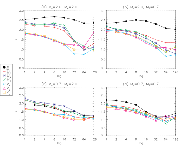
Figure 2.— Values of the $q$ parameter from the fits shown in Figure 1, the symbols (and colors) indicate the MHD variable used, according to the legend at the left of the plots.

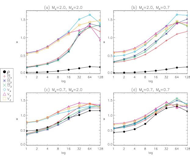
Figure 3.— Values of the $w$ parameter from the fits shown in Figure 1, the symbols (and colors) indicate the MHD variable used, according to the legend at the left of the plots.

In Figures 2 and 3 we see the same general trends found in solar wind studies (Burlaga & Viñas, 2004a, b, 2005a, 2005b; Burlaga et al., 2006a, b; Burlaga & Viñas, 2006; Burlaga et al., 2007a, b, 2009) and electron MHD simulations (Cho & Lazarian, 2009): a $q$ parameter that decreases, along with a $w$ value that increases as we take larger separations. In other words, the PDFs become more kurtotic, and narrower, as we go to small scales, while at large scales the PDFs are more Gaussian and wider. The same behavior (i.e. a decreasing kurtosis for an increasing lag) has been found also for velocity centroids in simulations and observations (see Falgarone et al., 1994; Lis et al., 1998; Klessen, 2000; Federrath et al., 2009). In fact, we have computed the kurtosis and variance of the PDFs (not shown here) and found a similar monotonic decrease and increase, respectively. Both the kurtosis and $q$ tend to their Gaussian value ($3$ and $1$, respectively) as the separation tends to the injection scale.

It is noticeable that the density PDFs in the supersonic regime have a very distinct shape than those of the velocity and magnetic field components. In the models of supersonic turbulence they are much narrower, and more peaked than in subsonic turbulence. They also show a shallower slope in the $q$ and $w$ vs $r$ plots. We can also notice slightly larger values of $q$ (and lower $w$) for the velocity components with respect to the magnetic field components, more pronounced for high Alfén Mach numbers.

5. Statistics of observable data: column density

The measures of non-Gaussianity presented in the previous section are interesting in their own right, and might provide us with insights to the intermittency of MHD turbulence from simulations. However, observations of the ISM cannot provide direct three-dimensional information of the density, velocity, and magnetic fields. For instance, from spectroscopic observations we can access only the velocity distribution of the emitting material at a given position (or positions) in the plane of the sky.

With the simulations presented in the previous section we have constructed (2D) maps of column density, assuming that the emitting material is optically thin, and with an emissivity linearly proportional to the density (e.g. H I). From the two-dimensional column density maps we constructed PDFs of column density increments, and following the same procedure we described before, we made fits to Tsallis distributions. The PDFs and the fits are presented in Figure 4.

Figure 4.— PDFs of column density fluctuations for different spatial separations (“x” symbols), and Tsallis fits (solid lines).

From the figure we can confirm the same general behavior of the PDFs, which become more Gaussian as we take larger separations. We can see that the PDFs are still consistent with Tsallis distributions, although the dependence on the lag is more subtle than with the 3D fields used in the previous section.

In Figure 5 we present the parameters $q$ and $w$ as obtained from the fitting procedure. Both panels of Figure 5 confirm the decrease of $q$ along with an increase of the width of the PDFs ($w$) with the lag. From the figure it is also evident that the fitting parameters can clearly distinguish between the supersonic and subsonic models. However, this can be done with other measures, for instance the variance of density or column density (Padoan et al., 1997; Passot & Vázquez-Semadeni, 2003; Federrath et al., 2008, 2009), or the skewness and kurtosis of density and column density PDFs (Kowal et al., 2007; Burkhart et al., 2009).

Figure 5.— Parameters q and w from d the Tsallis distribution fits shown in Figure 4.

A more difficult task is to extract information of the Alfvén Mach number. One can see from Figure 5 that the Tsallis parameters depend strongly on the sonic Mach number, and less so on the Alfvén Mach number. However, an encouraging clear dependence on the Alfvén Mach number is evident in the supersonic models, in particular for $w$ (lower panel of Figure 5), where all the $\mathcal{M}_{A}=2$ points lie above the $\mathcal{M}_{A}=0.7$ ones. But, for the subsonic models ($\mathcal{M}_{s}=0.7$) it not clear at all, and the behavior with the Alfén Mach number is the opposite, higher $w$ values for sub-alfvénic models.

6. Discussion

We found that the Tsallis expression [see Eq. (1)] describes well the statistics of the PDFs of our 3D-MHD numerical simulations. This is welcome news for both the ISM, where we propose to use Eq. (1) as a new tool to study turbulence, and for the solar wind studies, where the Tsallis expression was used, but its numerical testing was limited.

We have to add that the present work is intended only as a proof of concept. While the Tsallis PDFs do provide physical grounds to interpret the distributions obtained in MHD simulations and/or observations, it is not clear whether the formalism of non-extensive statistical dynamics is applicable to the turbulent ISM. This, we feel deserve a separate study. However, the fact that the expression provides both the fit to numerical MHD simulations and experimental data, and moreover seems to distinguish the Alfvén Mach number in some cases, is encouraging.

In regard to observational quantities, we should note that PDFs of velocity centroids (as opposed to column density, which is what we ave used in the present paper) have been employed to characterize the intermittency both in numerical models (Falgarone et al., 1994; Klessen, 2000; Federrath et al., 2009) and molecular cloud observations (for instance $\rho$-Ophiuchi in Lis et al. 1998; Polaris and Taurus in Hily-Blant et al. 2008). There is always a trade off while choosing different quantities to measure turbulence. On the one hand velocity is a dynamical quantity that is easy to relate with turbulence theories, however (at least in the case of power-spectra) is trickier to obtain, and in fact (for power-spectra) velocity centroids fail to trace the velocity statistics in strongly supersonic turbulence (see for instance Esquivel & Lazarian, 2005). On the other hand density fluctuations are not only produced from turbulence, but are more robustly obtained from observations (e.g. Lazarian & Pogosyan, 2008). We must stress that the healthy approach is to use these tools, and others as well, as complementary.

The most important finding of this paper is the dependence of the $q$ and $w$ parameters entering Eq. (1) on both sonic and Alfvén Mach number of the turbulence. These numbers are essential for many astrophysical processes from star formation (see McKee & Ostriker, 2007), magnetic diffusion enabled by reconnection (Lazarian, 2005), propagation of heat (Narayan & Medvedev, 2001; Lazarian, 2006a), cosmic rays (Yan & Lazarian, 2004) and dust grains acceleration (Yan et al., 2004).

By now several ways of estimating the Alfvén and sonic Mach numbers have been proposed (see Kowal et al. 2007), all with their own limitations and uncertainties. Thus the new approach here based on Eq. (1) is a welcome addition to the existing tools.

We should add however, that a number of turbulence parameters, which are as important as these Mach numbers, are not being explored in this work. The scale of turbulence, for instance, has important consequences for star formation (e.g. Klessen et al., 2000; Mac Low & Klessen, 2004) as well as for dynamo theory (e.g. Brandenburg & Subramanian, 2005b, a; Hanasz et al., 2009)

7. Summary

We have used three-dimensional MHD simulations to study the distribution functions of increments of density, velocity, and magnetic field. In addition, we studied synthetic column density maps, which can be directly compared with observations. The results can be summarized as follows.

1. The PDFs of each of all the quantities is well described by a Tsallis distribution. Such distributions are symmetric, and characterized basically by three parameters: an amplitude $A$, a width $w$, and the entropic index $q$ that relates to the shape (large values yield peaked distributions, while with small values they approximate to a Gaussian).

2. The general trend of the PDFs for different increments are consistent with previous studies, of solar wind observations. That is, the PDFs are close to a Gaussian distribution for large separations, and become more kurtotic and narrower (i.e. a larger degree of intermittency) for small separations.

3. While the PDFs of (3D) density are quite similar to those of magnetic field and velocity in subsonic turbulence (regardless of Alfvén Mach number), for supersonic turbulence (also independently of $\mathcal{M}_{A}$) they are noticeable narrower and more peaked. That is, the fits of the PDFs to a Tsallis distribution have smaller $w$, and larger $q$ parameters.

4. The column density maps show smoother distributions compared to those of density in 3D, however, we found that the $q$ values are larger for supersonic turbulence (and lower $w$ as well), regardless of the Alfvén Mach number.

5. The $w$ parameter of the Tsallis fits to the PDFs of column density increments seems to show a sensitivity to the Alfvén Mach number, at least in the cases of supersonic turbulence. With the limited data set used here is hard to conclude if this behavior is general, and whether it is useful to study the magnetization of ISM turbulence. Clearly, future studies of the PDFs in ISM turbulence (with a wider parameter coverage) are necessary.

References

- Ballesteros-Paredes et al. (2007) Ballesteros-Paredes, J., Klessen, R. S., Mac Low, M.-M., & Vazquez-Semadeni, E. 2007, in Protostars and Planets V, ed. B. Reipurth, D. Jewitt, & K. Keil, 63–80
- Brandenburg & Subramanian (2005a) Brandenburg, A., & Subramanian, K. 2005a, Phys. Rep., 417, 1
- Brandenburg & Subramanian (2005b) —. 2005b, Astronomische Nachrichten, 326, 400
- Brunt & Heyer (2002) Brunt, C. M., & Heyer, M. H. 2002, ApJ, 566, 276
- Burkhart et al. (2009) Burkhart, B., Falceta-Gonçalves, D., Kowal, G., & Lazarian, A. 2009, ApJ, 693, 250
- Burkhart et al. (2010) Burkhart, B., Stanimirovic, S., Lazarian, A., & Kowal, G. 2010, ApJ, submitted
- Burlaga et al. (2006a) Burlaga, L. F., Ness, N. F., & Acuña, M. H. 2006a, ApJ, 642, 584
- Burlaga et al. (2007a) —. 2007a, ApJ, 668, 1246
- Burlaga et al. (2009) —. 2009, ApJ, 691, L82
- Burlaga & Viñas (2004a) Burlaga, L. F., & Viñas, A. F. 2004a, Geophys. Res. Lett., 31, 16807
- Burlaga & Viñas (2004b) —. 2004b, Journal of Geophysical Research (Space Physics), 109, 12107
- Burlaga & Viñas (2005a) —. 2005a, Physica A Statistical Mechanics and its Applications, 356, 375
- Burlaga & Viñas (2005b) —. 2005b, Journal of Geophysical Research (Space Physics), 110, 7110
- Burlaga & Viñas (2006) —. 2006, Physica A Statistical Mechanics and its Applications, 361, 173
- Burlaga et al. (2006b) Burlaga, L. F., Viñas, A. F., Ness, N. F., & Acuña, M. H. 2006b, ApJ, 644, L83
- Burlaga et al. (2007b) Burlaga, L. F., Viñas, A. F., & Wang, C. 2007b, Journal of Geophysical Research (Space Physics), 112, 7206
- Chepurnov et al. (2008) Chepurnov, A., Gordon, J., Lazarian, A., & Stanimirovic, S. 2008, ApJ, 688, 1021
- Chepurnov & Lazarian (2009) Chepurnov, A., & Lazarian, A. 2009, ApJ, 693, 1074
- Chepurnov et al. (2006) Chepurnov, A., Lazarian, A., Stanimirovic, S., Heiles, C., & Peek, J. E. G. 2006, ArXiv Astrophysics e-prints
- Cho & Lazarian (2009) Cho, J., & Lazarian, A. 2009, ApJ, 701, 236
- Dickman & Kleiner (1985) Dickman, R. L., & Kleiner, S. C. 1985, ApJ, 295, 479
- Elmegreen & Scalo (2004) Elmegreen, B. G., & Scalo, J. 2004, ARA&A, 42, 211
- Esquivel & Lazarian (2005) Esquivel, A., & Lazarian, A. 2005, ApJ, 631, 320
- Esquivel et al. (2007) Esquivel, A., Lazarian, A., Horibe, S., Cho, J., Ossenkopf, V., & Stutzki, J. 2007, MNRAS, 381, 1733
- Esquivel et al. (2003) Esquivel, A., Lazarian, A., Pogosyan, D., & Cho, J. 2003, MNRAS, 342, 325
- Falgarone et al. (2005) Falgarone, E., Hily-Blant, P., Pety, J., & Pineau Des Forêts, G. 2005, in American Institute of Physics Conference Series, Vol. 784, Magnetic Fields in the Universe: From Laboratory and Stars to Primordial Structures., ed. E. M. de Gouveia dal Pino, G. Lugones, & A. Lazarian, 299–307
- Falgarone et al. (1994) Falgarone, E., Lis, D. C., Phillips, T. G., Pouquet, A., Porter, D. H., & Woodward, P. R. 1994, ApJ, 436, 728
- Federrath et al. (2009) Federrath, C., Duval, J., Klessen, R., Schmidt, W., & Mac Low, M. . 2009, ArXiv e-prints
- Federrath et al. (2008) Federrath, C., Klessen, R. S., & Schmidt, W. 2008, ApJ, 688, L79
- Hanasz et al. (2009) Hanasz, M., Otmianowska-Mazur, K., Kowal, G., & Lesch, H. 2009, A&A, 498, 335
- Henriksen (1994) Henriksen, R. N. 1994, Ap&SS, 221, 25
- Heyer & Schloerb (1997) Heyer, M. H., & Schloerb, F. P. 1997, ApJ, 475, 173
- Hily-Blant et al. (2008) Hily-Blant, P., Falgarone, E., & Pety, J. 2008, A&A, 481, 367
- Kim & Park (2007) Kim, S., & Park, C. 2007, ApJ, 663, 244
- Kleiner & Dickman (1985) Kleiner, S. C., & Dickman, R. L. 1985, ApJ, 295, 466
- Klessen (2000) Klessen, R. S. 2000, ApJ, 535, 869
- Klessen et al. (2000) Klessen, R. S., Heitsch, F., & Mac Low, M. 2000, ApJ, 535, 887
- Kowal et al. (2007) Kowal, G., Lazarian, A., & Beresnyak, A. 2007, ApJ, 658, 423
- Larson (1981) Larson, R. B. 1981, MNRAS, 194, 809
- Larson (1992) —. 1992, MNRAS, 256, 641
- Lazarian (2005) Lazarian, A. 2005, in American Institute of Physics Conference Series, Vol. 784, Magnetic Fields in the Universe: From Laboratory and Stars to Primordial Structures., ed. E. M. de Gouveia dal Pino, G. Lugones, & A. Lazarian, 42–53
- Lazarian (2006a) Lazarian, A. 2006a, ApJ, 645, L25
- Lazarian (2006b) Lazarian, A. 2006b, in American Institute of Physics Conference Series, Vol. 874, Spectral Line Shapes: XVIII, ed. E. Oks & M. S. Pindzola, 301–315
- Lazarian (2009) —. 2009, Space Science Reviews, 143, 357
- Lazarian & Esquivel (2003) Lazarian, A., & Esquivel, A. 2003, ApJ, 592, L37
- Lazarian & Pogosyan (2000) Lazarian, A., & Pogosyan, D. 2000, ApJ, 537, 720
- Lazarian & Pogosyan (2004) —. 2004, ApJ, 616, 943
- Lazarian & Pogosyan (2006) —. 2006, ApJ, 652, 1348
- Lazarian & Pogosyan (2008) —. 2008, ApJ, 686, 350
- Lazarian et al. (2002) Lazarian, A., Pogosyan, D., & Esquivel, A. 2002, in Astronomical Society of the Pacific Conference Series, Vol. 276, Seeing Through the Dust: The Detection of HI and the Exploration of the ISM in Galaxies, ed. A. R. Taylor, T. L. Landecker, & A. G. Willis, 182–+
- Lazarian et al. (2001) Lazarian, A., Pogosyan, D., Vázquez-Semadeni, E., & Pichardo, B. 2001, ApJ, 555, 130
- Leubner (2002) Leubner, M. P. 2002, Ap&SS, 282, 573
- Lis et al. (1998) Lis, D. C., Keene, J., Li, Y., Phillips, T. G., & Pety, J. 1998, ApJ, 504, 889
- Lis et al. (1996) Lis, D. C., Pety, J., Phillips, T. G., & Falgarone, E. 1996, ApJ, 463, 623
- Mac Low & Klessen (2004) Mac Low, M.-M., & Klessen, R. S. 2004, Reviews of Modern Physics, 76, 125
- Maksimovic et al. (1997) Maksimovic, M., Pierrard, V., & Riley, P. 1997, Geophys. Res. Lett., 24, 1151
- McKee & Ostriker (2007) McKee, C. F., & Ostriker, E. C. 2007, ARA&A, 45, 565
- Miesch & Bally (1994) Miesch, M. S., & Bally, J. 1994, ApJ, 429, 645
- Miesch et al. (1999) Miesch, M. S., Scalo, J., & Bally, J. 1999, ApJ, 524, 895
- Miesch & Scalo (1995) Miesch, M. S., & Scalo, J. M. 1995, ApJ, 450, L27
- Münch (1958) Münch, G. 1958, Reviews of Modern Physics, 30, 1035
- Narayan & Goodman (1989) Narayan, R., & Goodman, J. 1989, MNRAS, 238, 963
- Narayan & Medvedev (2001) Narayan, R., & Medvedev, M. V. 2001, ApJ, 562, L129
- O’Dell & Castaneda (1987) O’Dell, C. R., & Castaneda, H. O. 1987, ApJ, 317, 686
- Ossenkopf et al. (2006) Ossenkopf, V., Esquivel, A., Lazarian, A., & Stutzki, J. 2006, A&A, 452, 223
- Padoan et al. (2003) Padoan, P., Boldyrev, S., Langer, W., & Nordlund, Å. 2003, ApJ, 583, 308
- Padoan et al. (1997) Padoan, P., Jones, B. J. T., & Nordlund, A. P. 1997, ApJ, 474, 730
- Padoan et al. (2009) Padoan, P., Juvela, M., Kritsuk, A. G., & Norman, M. L. 2009, ArXiv e-prints
- Padoan et al. (2001) Padoan, P., Rosolowsky, E. W., & Goodman, A. A. 2001, ApJ, 547, 862
- Passot & Vázquez-Semadeni (2003) Passot, T., & Vázquez-Semadeni, E. 2003, A&A, 398, 845
- Press et al. (1992) Press, W. H., Teukolsky, S. A., Vetterling, W. T., & Flannery, B. P. 1992, Numerical recipes in FORTRAN. The art of scientific computing (Cambridge University Press)
- Rosolowsky et al. (1999) Rosolowsky, E. W., Goodman, A. A., Wilner, D. J., & Williams, J. P. 1999, ApJ, 524, 887
- Scalo (1984) Scalo, J. M. 1984, ApJ, 277, 556
- Scalo (1987) Scalo, J. M. 1987, in Astrophysics and Space Science Library, Vol. 134, Interstellar Processes, ed. D. J. Hollenbach & H. A. Thronson, Jr., 349–392
- Schmidt et al. (2009) Schmidt, W., Federrath, C., Hupp, M., Kern, S., & Niemeyer, J. C. 2009, A&A, 494, 127
- Schmidt et al. (2008) Schmidt, W., Federrath, C., & Klessen, R. 2008, Physical Review Letters, 101, 194505
- She & Lévêque (1994) She, Z.-S., & Lévêque, E. 1994, Phys. Rev. Lett., 72, 336
- Spangler & Gwinn (1990) Spangler, S. R., & Gwinn, C. R. 1990, ApJ, 353, L29
- Stutzki et al. (1998) Stutzki, J., Bensch, F., Heithausen, A., Ossenkopf, V., & Zielinsky, M. 1998, A&A, 336, 697
- Tsallis (1988) Tsallis, C. 1988, Journal of Statistical Physics, 52, 479
- von Hoerner (1951) von Hoerner, S. 1951, Zeitschrift fur Astrophysik, 30, 17
- Yan & Lazarian (2004) Yan, H., & Lazarian, A. 2004, ApJ, 614, 757
- Yan et al. (2004) Yan, H., Lazarian, A., & Draine, B. T. 2004, ApJ, 616, 895