A sticky HDP-HMM with application to speaker diarization

Abstract

We consider the problem of speaker diarization, the problem of segmenting an audio recording of a meeting into temporal segments corresponding to individual speakers. The problem is rendered particularly difficult by the fact that we are not allowed to assume knowledge of the number of people participating in the meeting. To address this problem, we take a Bayesian nonparametric approach to speaker diarization that builds on the hierarchical Dirichlet process hidden Markov model (HDP-HMM) of Teh et al. [J. Amer. Statist. Assoc. 101 (2006) 1566–1581]. Although the basic HDP-HMM tends to over-segment the audio data—creating redundant states and rapidly switching among them—we describe an augmented HDP-HMM that provides effective control over the switching rate. We also show that this augmentation makes it possible to treat emission distributions nonparametrically. To scale the resulting architecture to realistic diarization problems, we develop a sampling algorithm that employs a truncated approximation of the Dirichlet process to jointly resample the full state sequence, greatly improving mixing rates. Working with a benchmark NIST data set, we show that our Bayesian nonparametric architecture yields state-of-the-art speaker diarization results.

T2Supported in part by MURIs funded through AFOSR Grant FA9550-06-1-0324 and ARO Grant W911NF-06-1-0076, by AFOSR under Grant FA9559-08-1-0180 and by DARPA IPTO Contract FA8750-05-2-0249.

, , and

1 Introduction

A recurring problem in many areas of information technology is that of segmenting a waveform into a set of time intervals that have a useful interpretation in some underlying domain. In this article we focus on a particular instance of this problem, namely, the problem of speaker diarization. In speaker diarization, an audio recording is made of a meeting involving multiple human participants and the problem is to segment the recording into time intervals associated with individual speakers [Wooters and Huijbregts (2007)]. This segmentation is to be carried out without a priori knowledge of the number of speakers involved in the meeting; moreover, we do not assume that we have a priori knowledge of the speech patterns of particular individuals.

Our approach to the speaker diarization problem is built on the framework of hidden Markov models (HMMs), which have been a major success story not only in speech technology but also in many other fields involving complex sequential data, including genomics, structural biology, machine translation, cryptanalysis and finance. An alternative to HMMs in the speaker diarization setting would be to treat the problem as a changepoint detection problem, but a key aspect of speaker diarization is that speech data from a single individual generally recurs in multiple disjoint intervals. This suggests a Markovian framework in which the model transitions among states that are associated with the different speakers.

An apparent disadvantage of the HMM framework, however, is that classical treatments of the HMM generally require the number of states to be fixed a priori. While standard parametric model selection methods can be adapted to the HMM, there is little understanding of the strengths and weaknesses of such methods in this setting, and practical applications of HMMs generally fix the number of states using ad hoc approaches. It is not clear how to adapt HMMs to the diarization problem where the number of speakers is unknown.

Building on the work of Beal, Ghahramani and Rasmussen (2002), Teh et al. (2006) presented a Bayesian nonparametric version of the HMM in which a stochastic process—the hierarchical Dirichlet process (HDP)—defines a prior distribution on transition matrices over countably infinite state spaces. The resulting HDP-HMM is amenable to full Bayesian posterior inference over the number of states in the model. Moreover, this posterior distribution can be integrated over when making predictions, effectively averaging over models of varying complexity. The HDP-HMM has shown promise in a variety of applied problems, including visual scene recognition [Kivinen, Sudderth and Jordan (2007)], music synthesis [Hoffman, Cook and Blei (2008)], and the modeling of genetic recombination [Xing and Sohn (2007)] and gene expression [Beal and Krishnamurthy (2006)].

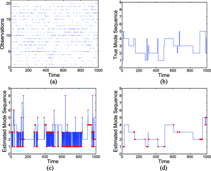
Figure 1: (a) Multinomial observation sequence; (b) true state sequence; (c) and (d) estimated state sequence after 30,000 Gibbs iterations for the original and sticky HDP-HMM, respectively, with errors indicated in red. Without an extra self-transition bias, the HDP-HMM rapidly transitions among redundant states.

While the HDP-HMM seems like a natural fit to the speaker diarization problem given its structural flexibility, as we show in Section 8, the HDP-HMM does not yield state-of-the-art performance in the speaker diarization setting. The problem is that the HDP-HMM inadequately models the temporal persistence of states. This problem arises in classical finite HMMs as well, where semi-Markovian models are often proposed as solutions. However, the problem is exacerbated in the nonparametric setting, in which the Bayesian bias toward simpler models is insufficient to prevent the HDP-HMM from giving high posterior probability to models with unrealistically rapid switching. This is demonstrated in Figure 1, where we see that the HDP-HMM sampling algorithm creates redundant states and rapidly switches among them. (The figure also displays results from the augmented HDP-HMM—the “sticky HDP-HMM” that we describe in this paper.) The tendency to create redundant states is not necessarily a problem in settings in which model averaging is the goal. For speaker diarization, however, it is critical to infer the number of speakers as well as the transitions among speakers.

Thus, one of our major goals in this paper is to provide a general solution to the problem of state persistence in HDP-HMMs. Our approach is easily stated—we simply augment the HDP-HMM to include a parameter for self-transition bias, and place a separate prior on this parameter. The challenge is to execute this idea coherently in a Bayesian nonparametric framework. Earlier papers have also proposed self-transition parameters for HMMs with infinite state spaces [Beal, Ghahramani and Rasmussen (2002); Xing and Sohn (2007)], but did not formulate general solutions that integrate fully with Bayesian nonparametric inference.

Another goal of the current paper is to develop a more fully nonparametric version of the HDP-HMM in which not only the transition distribution but also the emission distribution (the conditional distribution of observations given states) is treated nonparametrically. This is again motivated by the speaker diarization problem—in classical applications of HMMs to speech recognition problems, it is often the case that emission distributions are found to be multimodal, and high-performance HMMs generally use finite Gaussian mixtures as emission distributions [Gales and Young (2007)]. In the nonparametric setting it is natural to replace these finite mixtures with Dirichlet process mixtures. Unfortunately, this idea is not viable in practice, because of the tendency of the HDP-HMM to rapidly switch between redundant states. As we show, however, by incorporating an additional self-transition bias, it is possible to make use of Dirichlet process mixtures for the emission distributions.

An important reason for the popularity of the classical HMM is its computational tractability. In particular, marginal probabilities and samples can be obtained from the HMM via an efficient dynamic programming algorithm known as the forward–backward algorithm [Rabiner (1989)]. We show that this algorithm also plays an important role in computationally efficient inference for our generalized HDP-HMM. Using a truncated approximation to the full Bayesian nonparametric model, we develop a blocked Gibbs sampler which leverages forward–backward recursions to jointly resample the state and emission assignments for all observations.

The paper is organized as follows. In Section 2 we begin by summarizing related prior work on the speaker diarization task and analyzing the key characteristics of the data set we examine in Section 8. In Section 3 we provide some basic background on Dirichlet processes. Then, in Section 4 we overview the hierarchical Dirichlet process, and in Section 5 discuss how it applies to HMMs and can be extended to account for state persistence. An efficient Gibbs sampler is also described in this section. In Section 7 we treat the case of nonparametric emission distributions. We discuss our application to speaker diarization in Section 8. A list of notational conventions can be found in the Supplementary Material [Fox et al. (2010)].

2 The speaker diarization task

There is a vast literature on the speaker diarization task, and in this section we simply aim to provide an overview of the most common techniques. We refer the interested reader to Tranter and Reynolds (2006) for a more thorough exposition on the subject.

Classical speaker diarization techniques typically employ a two-stage procedure that first segments the audio (or features thereof) using one of a variety of changepoint algorithms. The inferred segments are then regrouped into a set of speaker labels via a clustering algorithm. For example, Reynolds and Torres-Carrasquillo (2004) propose a changepoint detection method based on the Bayesian Information Criterion (BIC). Specifically, a penalized likelihood ratio test is used to compare whether the data within a fixed window are better modeled via a single Gaussian or two Gaussians. The window gradually grows at each test until a changepoint is inferred, at which point the window is reinitialized at the inferred changepoint. An alternative changepoint detection technique, first proposed in Siegler et al. (1997), uses fixed length windows and computes the symmetric Kullback–Leibler (KL) divergence between a pair of Gaussians each fit by the data in their respective windows. A post-processing step then sets the changepoints equal to the peaks of the computed KL that exceed a predetermined threshold. In order to group the inferred segments into a set of speaker labels, a common approach is to use hierarchical agglomerative clustering with a BIC stopping criterion, as proposed in Chen and Gopalakrishnam (1998).

The simple two-stage approach outlined above suffers from the fact that errors made in the segmentation stage can degrade the performance of the subsequent clustering stage. A number of algorithms instead iterate between multiple stages of resegmentation (typically via Viterbi decoding) and clustering; for example, see Barras et al. (2004); Wooters et al. (2004). Iterative segmentation and clustering algorithms employing a Gaussian mixture model for each cluster (i.e., speaker), such as those proposed by Gauvain, Lamel and Adda (1998); Barras et al. (2004), have been shown to improve diarization performance. Overall, however, agglomerative clustering is extremely sensitive to the specified threshold for cluster merging, with different settings leading to either over- or under-clustering of the segments into speakers. The thresholds are typically set based on testing on an extensive training database.

A number of more recent approaches have considered the problem of joint segmentation and clustering by employing HMMs to capture the repeated returns of speakers. To handle the fact that the state space is unknown, Meignier et al. (2000) introduces the use of an evolutive-HMM which is further developed in Meignier, Bonastre and Igounet (2001). The HMM is initialized to have one state and at each iteration a segment of speech is assumed to arise from an undetected speaker who is added to the model. The revised HMM is then used to resegment the audio, and this iterative procedure continues until the speaker labels have converged. An alternative HMM formulation is presented in Wooters and Huijbregts (2007). The data are initially split into $K$ states, with $K$ assumed to be larger than the number of true speakers, and the HMM states are iteratively merged according to a metric based on changes in BIC. At each iteration, Viterbi decoding is performed to resegment the features of the audio, and the inferred segments are used to fit a new HMM via expectation maximization (EM). Then, the BIC criterion is applied to decide whether to merge HMM states. The algorithm also includes HMM substates to impose minimum speaker durations.

Our approach also seeks to jointly segment and cluster the audio into speaker-homogenous regions, as targeted by the HMM approaches of Meignier, Bonastre and Igounet (2001); Wooters and Huijbregts (2007), but within a Bayesian nonparametric framework that avoids relying on the heuristics employed by these previously proposed algorithms and allows for coherent Bayesian inference.

The data set we consider in the experiments of Section 8 is a standard benchmark data set distributed by NIST as part of the Rich Transcription 2004–2007 meeting recognition evaluations [NIST (2007)]. The data set consists of 21 recorded meetings, each of which may have different sets of speakers both in number and identity. We use the first 19 Mel Frequency Cepstral Coefficients (MFCCs), computed over a 30 ms window every 10 ms, as a feature vector. After these features are computed, a speech/nonspeech detector is run to identify and remove observations corresponding to nonspeech. (Nonspeech refers to time intervals in which nobody is speaking.) The preprocessing step of removing nonspeech observations is important in ensuring that the fitted acoustic models are not corrupted by nonspeech information.

When working with this data set, we discovered that the high frequency content of these features contained little discriminative information. Since minimum speaker durations are rarely less than 500 ms, we chose to define the observations as averages over 250 ms, nonoverlapping blocks. This preprocessing stage also aids in achieving speaker dynamics at the correct granularity (as opposed to finer temporal scale features leading to inferring within-speaker dynamics in addition to global speaker changes). In Figure 2 we plot a histogram of the speaker durations of our preprocessed features based on the ground truth labels provided for each of the 21 meetings. From this plot, we see that a geometric duration distribution fits this data reasonably well. This motivates our approach of simply increasing the prior probability of self-transitions within a Markov framework rather than moving to the more complicated semi-Markov formulation of speaker transitions.

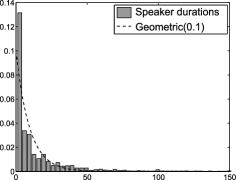
Figure 2: Normalized histogram of speaker durations of the preprocessed audio features from the 21 meetings in the NIST database. A $\operatorname{Geom}(0.1)$ density is also shown for comparison.

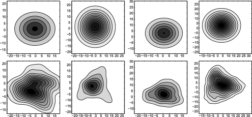
Figure 3: Contour plots of the best fit Gaussian (top) and kernel density estimate (bottom) for the top two principal components of the audio features associated with each of the four speakers present in the AMI_20041210-1052 meeting. Without capturing the non-Gaussianity of the speaker-specific emissions, the speakers are challenging to identify.

Another key feature of the speaker diarization data is the fact that the speaker specific emissions are not well approximated by a single Gaussian; see Figure 3. This observation has led many researchers to consider a mixture-of-Gaussians speaker model, as previously described. As demonstrated in Section 8, we show that achieving state-of-the-art performance within our framework also relies on allowing for non-Gaussian emissions.

3 Dirichlet processes

A Dirichlet process (DP) is a distribution on probability measures on a measurable space $\Theta$. This stochastic process is uniquely defined by a base measure $H$ on $\Theta$ and a concentration parameter $\gamma$; we denote it by $\operatorname{DP}({\gamma},{H})$. Consider a random probability measure $G_{0}\sim\operatorname{DP}({\gamma},{H})$. The DP is formally defined by the property that, for any finite partition $\{A_{1},\dots,A_{K}\}$ of $\Theta$,

$$(G_{0}(A_{1}),\dots,G_{0}(A_{K}))|\gamma,H\sim\operatorname{Dir}(\gamma H(A_{1}),\dots,\gamma H(A_{K})).\vspace*{-1pt}$$ (1)

That is, the measure of a random probability distribution $G_{0}\sim\operatorname{DP}({\gamma},{H})$ on every finite partition of $\Theta$ follows a finite-dimensional Dirichlet distribution [Ferguson (1973)]. A more constructive definition of the DP was given by Sethuraman (1994). Consider a probability mass function (p.m.f.) $\{\beta_{k}\}_{k=1}^{\infty}$ on a countably infinite set, where the discrete probabilities are defined as follows:

$$v_{k}|\gamma \sim \operatorname{Beta}(1,\gamma),\qquad k=1,2,\dots,$$

$$\beta_{k} = v_{k}\prod_{\ell=1}^{k-1}(1-v_{\ell}),\qquad k=1,2,\dots.\vspace*{-3pt}$$

In effect, we have divided a unit-length stick into lengths given by the weights $\beta_{k}$: the $k$th weight is a random proportion $v_{k}$ of the remaining stick after the previous $(k-1)$ weights have been defined. This stick-breaking construction is generally denoted by $\beta\sim\operatorname{GEM}(\gamma)$. With probability one, a random draw $G_{0}\sim\operatorname{DP}(\gamma,H)$ can be expressed as

$$G_{0}=\sum_{k=1}^{\infty}\beta_{k}\delta_{\theta_{k}},\qquad\theta_{k}|H\sim H,k=1,2,\dots,\vspace*{-3pt}$$ (3)

where $\delta_{\theta}$ denotes a unit-mass measure concentrated at $\theta$ and where $\{\theta_{k}\}$ are drawn independently from $H$. From this definition, we see that the DP actually defines a distribution over discrete probability measures. The stick-breaking construction also gives us insight into how the concentration parameter $\gamma$ controls the relative magnitude of the mixture weights $\beta_{k}$, and thus determines the model complexity in terms of the expected number of components with significant probability mass.

The DP has a number of properties which make inference based on this nonparametric prior computationally tractable. Consider a set of observations $\{\theta^{\prime}_{i}\}$ with $\theta^{\prime}_{i}\sim G_{0}$. Because probability measures drawn from a DP are discrete, there is a strictly positive probability of multiple observations $\theta^{\prime}_{i}$ taking identical values within the set $\{\theta_{k}\}$, with $\theta_{k}$ defined as in equation (3). For each value $\theta^{\prime}_{i}$, let $z_{i}$ be an indicator random variable that picks out the unique value $k$ such that $\theta^{\prime}_{i}=\theta_{z_{i}}$. Blackwell and MacQueen (1973) introduced a Pólya urn representation of the $\theta^{\prime}_{i}$:

$$\theta^{\prime}_{i}|\theta^{\prime}_{1},\dots,\theta^{\prime}_{i-1} \sim \frac{\gamma}{\gamma+i-1}H+\sum_{j=1}^{i-1}\frac{1}{\gamma+i-1}\delta_{\theta^{\prime}_{j}}$$

$$= \frac{\gamma}{\gamma+i-1}H+\sum_{k=1}^{K}\frac{n_{k}}{\gamma+i-1}\delta_{\theta_{k}},\vspace*{-3pt}$$

implying the following predictive distribution for the indicator random variables:

$$\qquad\ \ p(z_{N+1}=z|z_{1},\dots,z_{N},\gamma)=\frac{\gamma}{N+\gamma}\delta(z,K+1)+\frac{1}{N+\gamma}\sum_{k=1}^{K}n_{k}\delta(z,k).\vspace*{-3pt}$$ (5)

Here, $n_{k}=\sum_{i=1}^{N}\delta(z_{i},k)$ is the number of indicator random variables taking the value $k$, and $K+1$ is a previously unseen value. We use the notation $\delta(z,k)$ to indicate the discrete Kronecker delta. This representation can be used to sample observations from a DP without explicitly constructing the countably infinite random probability measure $G_{0}\sim\operatorname{DP}({\gamma},{H})$.

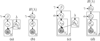
Figure 4: Dirichlet process (left) and hierarchical Dirichlet process (right) mixture models represented in two different ways as graphical models. (a) Indicator variable representation in which $\beta|\gamma\sim\operatorname{GEM}(\gamma)$, $\theta_{k}|H,\lambda\sim H(\lambda)$, $z_{i}|\beta\sim\beta$ and $y_{i}|\{\theta_{k}\}_{k=1}^{\infty},z_{i}\sim F(\theta_{z_{i}})$. (b) Alternative representation with $G_{0}|\gamma,H\sim\operatorname{DP}({\gamma},{H})$, $\theta^{\prime}_{i}|G_{0}\sim G_{0}$, and $y_{i}|\theta^{\prime}_{i}\sim F(\theta^{\prime}_{i})$. (c) Indicator variable representation in which $\beta|\gamma\sim\operatorname{GEM}(\gamma)$, $\pi_{k}|\alpha,\beta\sim\operatorname{DP}({\alpha},{\beta})$, $\theta_{k}|H,\lambda\sim H(\lambda)$, $z_{ji}|\pi_{j}\sim\pi_{j}$, and $y_{ji}|\{\theta_{k}\}_{k=1}^{\infty},z_{ji}\sim F(\theta_{z_{ji}})$. (d) Alternative representation with $G_{0}|\gamma,H\sim\operatorname{DP}({\gamma},{H})$, $G_{j}|G_{0}\sim\operatorname{DP}({\alpha},{G_{0}})$, $\theta^{\prime}_{ji}|G_{j}\sim G_{j}$ and $y_{ji}|\theta^{\prime}_{ji}\sim F(\theta^{\prime}_{ji})$. The “plate” notation is used to compactly represent replication [Teh et al. (2006)].

The distribution on partitions induced by the sequence of conditional distributions in equation (5) is commonly referred to as the Chinese restaurant process. The analogy, which is useful in developing various generalizations of the Dirichlet process we consider in this paper, is as follows. Take $i$ to be a customer entering a restaurant with infinitely many tables, each serving a unique dish $\theta_{k}$. Each arriving customer chooses a table, indicated by $z_{i}$, in proportion to how many customers are currently sitting at that table. With some positive probability proportional to $\gamma$, the customer starts a new, previously unoccupied table $K+1$. The Chinese restaurant process captures the fact that the DP has a clustering property such that multiple draws from the random measure take the same value.

The DP is commonly used as a prior on the parameters of a mixture model with a random number of components. Such a model is called a Dirichlet process mixture model and is depicted as a graphical model in Figure 4(a) and (b). To generate observations, we choose $\theta^{\prime}_{i}\sim G_{0}$ and $y_{i}\sim F(\theta^{\prime}_{i})$ for an indexed family of distributions $F(\cdot)$. This sampling process is also often described in terms of the indicator random variables $z_{i}$; in particular, we have $z_{i}\sim\beta$ and $y_{i}\sim F(\theta_{z_{i}})$. The parameter with which an observation is associated implicitly partitions or clusters the data. In addition, the Chinese restaurant process representation indicates that the DP provides a prior that makes it more likely to associate an observation with a parameter to which other observations have already been associated. This reinforcement property is essential for inferring finite, compact mixture models. It can be shown under mild conditions that if the data were generated by a finite mixture, then the DP posterior is guaranteed to converge (in distribution) to that finite set of mixture parameters [Ishwaran and Zarepour (2002b)].

4 Hierarchical Dirichlet processes

In the following section we describe how ideas based on the Dirichlet process have been used to develop a Bayesian nonparametric approach to hidden Markov modeling in which the number of states is unknown a priori. To develop this nonparametric version of the HMM, the Dirichlet process does not suffice; rather, it is necessary to develop a hierarchical Bayesian model involving a tied collection of Dirichlet processes. This has been done by Teh et al. (2006) whose hierarchical Dirichlet process (HDP) we describe in this section. The HDP is applicable to general problems involving related groups of data, each of which can be modeled using a DP, and we begin by describing the HDP at this level of generality, subsequently specializing to the HMM.

To describe the HDP, suppose there are $J$ groups of data and let $\{y_{j1},\dots,\break y_{j{N_{j}}}\}$ denote the set of observations in group $j$. Assume that there are a collection of DP mixture models underlying the observations in these groups:

$$G_{j} = \sum_{t=1}^{\infty}\tilde{\pi}_{jt}\delta_{\theta^{*}_{jt}},\qquad\tilde{\pi}_{j}|\alpha\sim\operatorname{GEM}(\alpha),j=1,\ldots,J,$$ (6)

$$\qquad\hskip 51.0pt\theta^{*}_{jt}|G_{0},\sim G_{0},t=1,2,\ldots,$$

$$\qquad\theta^{\prime}_{ji}|G_{j} \sim G_{j},\qquad y_{ji}|\theta^{\prime}_{ji}\sim F(\theta^{\prime}_{ji}),\qquad j=1,\dots,J,i=1,\dots,N_{j}.$$

We wish to tie the DP mixtures across the different groups such that atoms that underly the data in group $j$ can be used in group $j^{\prime}$. The problem is that if $G_{0}$ is absolutely continuous with respect to the Lebesgue measure (as it generally is for continuous parameters), then the atoms in $G_{j}$ will be distinct from those in $G_{j^{\prime}}$ with probability one. The solution to this problem is to let $G_{0}$ itself be a draw from a DP:

$$G_{0}=\sum_{k=1}^{\infty}\beta_{k}\delta_{\theta_{k}},\qquad \beta|\gamma\sim\operatorname{GEM}(\gamma),$$

$$\theta_{k}|H,\lambda\sim H(\lambda),k=1,2,\dots.$$

In this hierarchical model, $G_{0}$ is atomic and random. Letting $G_{0}$ be a base measure for the draw $G_{j}\sim\operatorname{DP}({\alpha},{G_{0}})$ implies that only these atoms can appear in $G_{j}$. Thus, atoms can be shared among the collection of random measures $\{G_{j}\}$. The HDP model is depicted graphically in two different ways in Figure 4(c) and (d).

Teh et al. (2006) have also described the marginal probabilities obtained from integrating over the random measures $G_{0}$ and $\{G_{j}\}$. They show that these marginals can be described in terms of a Chinese restaurant franchise (CRF) that is an analog of the Chinese restaurant process. The CRF is comprised of $J$ restaurants, each corresponding to an HDP group, and an infinite buffet line of dishes common to all restaurants. The process of seating customers at tables, however, is restaurant specific. Each customer is preassigned to a given restaurant determined by that customer’s group $j$. Upon entering the $j$th restaurant in the CRF, customer $y_{ji}$ sits at currently occupied tables $t_{ji}$ with probability proportional to the number of currently seated customers, or starts a new table $T_{j}+1$ with probability proportional to $\alpha$. The first customer to sit at a table goes to the buffet line and picks a dish $k_{jt}$ for their table, choosing the dish with probability proportional to the number of times that dish has been picked previously, or ordering a new dish $\theta_{K+1}$ with probability proportional to $\gamma$. The intuition behind this predictive distribution is that integrating over the global dish probabilities $\beta$ results in customers making decisions based on the observed popularity of the dishes throughout the entire franchise. See the Supplementary Material for further details [Fox et al. (2010)].

Recalling equations (6) and (4), since each distribution $G_{j}$ is drawn from a DP with a discrete base measure $G_{0}$, multiple $\theta^{*}_{jt}$ may take an identical value $\theta_{k}$ for multiple unique values of $t$. As we see in the Supplemental Material [Fox et al. (2010)], this corresponds to multiple tables in the same restaurant being served the same dish. We can write $G_{j}$ as a function of the unique dishes:

$$G_{j}=\sum_{k=1}^{\infty}\pi_{jk}\delta_{\theta_{k}},\qquad\pi_{j}|\alpha,\beta\sim\operatorname{DP}({\alpha},{\beta}),\theta_{k}|H\sim H,\vspace*{-3pt}$$ (8)

where $\pi_{j}$ now defines a restaurant-specific distribution over dishes served rather than over tables, with

$$\pi_{jk}=\sum_{t|\theta^{*}_{jt}=\theta_{k}}\tilde{\pi}_{jt}.\vspace*{-3pt}$$ (9)

Let $z_{ji}$ be the indicator random variable for the unique dish selected by observation $y_{ji}$. An equivalent representation for the generative model is in terms of these indicator random variables:

$$\quad\pi_{j}|\alpha,\beta\sim\operatorname{DP}({\alpha},{\beta}),\qquad z_{ji}|\pi_{j}\sim\pi_{j},\qquad y_{ji}|\{\theta_{k}\},z_{ji}\sim F(\theta_{z_{ji}}),$$ (10)

and is shown in Figure 4(c).

5 The sticky HDP-HMM

Recall that the hidden Markov model, or HMM, is a class of doubly stochastic processes based on an underlying, discrete-valued state sequence, which is modeled as Markovian [Rabiner (1989)]. Let $z_{t}$ denote the state of the Markov chain at time $t$ and $\pi_{j}$ the state-specific transition distribution for state $j$. Then, the Markovian structure on the state sequence dictates that $z_{t}\sim\pi_{z_{t-1}}$. The observations, $y_{t}$, are conditionally independent given this state sequence, with $y_{t}\sim F(\theta_{z_{t}})$ for some fixed distribution $F(\cdot)$.

The HDP can be used to develop an HMM with an infinite state space—the HDP-HMM [Teh et al. (2006)]. In the speaker diarization task, each state constitutes a different speaker and our goal in moving to an infinite state space is to remove upper bounds on the total number of speakers present. Conceptually, we envision a doubly-infinite transition matrix, with each row corresponding to a Chinese restaurant. That is, the groups in the HDP formalism here correspond to states, and each Chinese restaurant defines a distribution on next states. The CRF links these next-state distributions. Thus, in this application of the HDP, the group-specific distribution, $\pi_{j}$, is a state-specific transition distribution and, due to the infinite state space, there are infinitely many such groups. Since $z_{t}\sim\pi_{z_{t-1}}$, we see that $z_{t-1}$ indexes the group to which $y_{t}$ is assigned (i.e., all observations with $z_{t-1}=j$ are assigned to group $j$). Just as with the HMM, the current state $z_{t}$ then indexes the parameter $\theta_{z_{t}}$ used to generate observation $y_{t}$ [see Figure 5(a)].

By defining $\pi_{j}\sim\operatorname{DP}({\alpha},{\beta})$, the HDP prior encourages states to have similar transition distributions ($E[\pi_{jk}|\beta]=\beta_{k}$). However, it does not differentiate self-transitions from moves between different states. When modeling data with state persistence, the flexible nature of the HDP-HMM prior allows for state sequences with unrealistically fast dynamics to have large posterior probability. For example, with multinomial emissions, a good explanation of the data is to divide different observation values into unique states and then rapidly switch between them (see Figure 1). In such cases, many models with redundant states may have large posterior probability, thus impeding our ability to identify a compact dynamical model which best explains the observations. The problem is compounded by the fact that once this alternating pattern has been instantiated by the sampler, its persistence is then reinforced by the properties of the Chinese restaurant franchise, thus slowing mixing rates. Furthermore, this fragmentation of data into redundant states can reduce predictive performance, as is discussed in Section 6. In many applications, one would like to be able to incorporate prior knowledge that slow, smoothly varying dynamics are more likely.

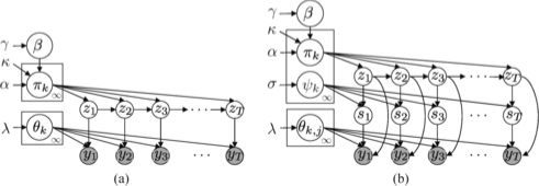
Figure 5: (a) Graphical representation of the sticky HDP-HMM. The state evolves as $z_{t+1}|\{\pi_{k}\}_{k=1}^{\infty},z_{t}\sim\pi_{z_{t}}$, where $\pi_{k}|\alpha,\kappa,\beta\sim\operatorname{DP}(\alpha+\kappa,(\alpha\beta+\kappa\delta_{k})/(\alpha+\kappa))$ and $\beta|\gamma\sim\operatorname{GEM}(\gamma)$, and observations are generated as $y_{t}|\{\theta_{k}\}_{k=1}^{\infty},z_{t}\sim F(\theta_{z_{t}})$. The original HDP-HMM has $\kappa=0$. (b) Sticky HDP-HMM with DP emissions, where $s_{t}$ indexes the state-specific mixture component generating observation $y_{t}$. The DP prior dictates that $s_{t}|\{\psi_{k}\}_{k=1}^{\infty},z_{t}\sim\psi_{z_{t}}$ for $\psi_{k}|\sigma\sim\operatorname{GEM}(\sigma)$. The $j$th Gaussian component of the $k$th mixture density is parameterized by $\theta_{k,j}$ so $y_{t}|\{\theta_{k,j}\}_{k,j=1}^{\infty},z_{t},s_{t}\sim F(\theta_{z_{t},s_{t}})$.

To address these issues, we propose to instead model the transition distributions $\pi_{j}$ as follows:

$$\beta|\gamma \sim \operatorname{GEM}(\gamma),$$

$$\pi_{j}|\alpha,\kappa,\beta \sim \operatorname{DP}\biggl{(}\alpha+\kappa,\frac{\alpha\beta+\kappa\delta_{j}}{\alpha+\kappa}\biggr{)}.$$

Here, $(\alpha\beta+\kappa\delta_{j})$ indicates that an amount $\kappa>0$ is added to the $j$th component of $\alpha\beta$. Informally, what we are doing is increasing the expected probability of self-transition by an amount proportional to $\kappa$:

$$E[\pi_{jk}|\beta,\kappa]=\frac{\alpha\beta_{k}+\kappa\delta(j,k)}{\alpha+\kappa}.$$ (12)

More formally, over a finite partition $(Z_{1},\dots,Z_{K})$ of the positive integers $\mathbb{Z}_{+}$, the prior on the measure $\pi_{j}$ adds an amount $\kappa$ only to the arbitrarily small partition containing $j$, corresponding to a self-transition. That is,

$$(\pi_{j}(Z_{1}),\dots,\pi_{j}(Z_{K}))|\alpha,\beta$$

(13)

$$\qquad\sim\operatorname{Dir}\bigl{(}\alpha\beta(Z_{1})+\kappa\delta_{j}(Z_{1}),\dots,\alpha\beta(Z_{K})+\kappa\delta_{j}(Z_{K})\bigr{)}.$$

When $\kappa=0$ the original HDP-HMM of Teh et al. (2006) is recovered. Because positive $\kappa$ values increase the prior probability $E[\pi_{jj}|\beta]$ of self-transitions, we refer to this extension as the sticky HDP-HMM. See Figure 5(a). Note that this formulation assumes that the stickiness of each HMM state is the same a priori. The parameter could be made state-dependent through a hierarchical model that ties together a collection of state-specific sticky parameters. However, such state-specific stickiness is unnecessary for the speaker diarization task at hand since each speaker is assumed to have similar expected durations. Differences between speaker-specific transitions become more distinguished in the posterior.

The $\kappa$ parameter is reminiscent of the self-transition bias parameter of the infinite HMM, an urn model for hidden Markov models on infinite state spaces that predated the HDP-HMM [Beal, Ghahramani and Rasmussen (2002)]. The connection between the (sticky) HDP-HMM and the infinite HMM is analogous to that between the DP and the Pólya urn; in both cases the latter is obtained by integrating out the random measures in the former. In particular, the infinite HMM employs a two-level urn model in which the top-level urn places a probability on transitions to existing states in proportion to how many times these transitions have been seen, with an added bias for a self-transition even if this has not previously occurred. With some remaining probability, an oracle is called, representing the second-level urn. This oracle chooses an existing state in proportion to how many times the oracle previously chose that state, regardless of the state transition involved, or chooses a previously unvisited state. The original HDP-HMM provides an interpretation of this urn model in terms of an underlying collection of linked random probability measures, however, without the self-transition parameter. In addition to the conceptual clarity provided by the random measure formalism, the HDP-HMM has the practical advantage that it makes it possible to use standard MCMC algorithms for posterior inference; working within the urn model formulation, Beal, Ghahramani and Rasmussen (2002) needed to resort to a heuristic approximation to a Gibbs sampler. The sticky HDP-HMM, an early version of which was presented in Fox et al. (2008), restores the self-transition parameter of the infinite HMM to this class of models, doing so in a way that integrates with a full Bayesian nonparametric specification.

As with the DP, this specification in terms of random measures yields various interesting characterizations of marginal probabilities. In particular, as described in the Supplemental Material [Fox et al. (2010)], the partitioning structure induced by the sticky HDP-HMM has an interpretation as an extension of the Chinese restaurant franchise (CRF) which we refer to as a CRF with loyal customers. Here, each restaurant in the franchise has a specialty dish with the same index as that of the restaurant. Although this dish is served elsewhere, it is more popular in the dish’s namesake restaurant. Recall that while customers in the CRF of the HDP are pre-partitioned into restaurants based on the fixed group assignments, in the HDP-HMM the value of the state $z_{t}$ determines the group assignment (and thus restaurant) of customer $y_{t+1}$. The increased popularity of the house specialty dish (determined by the sticky parameter $\kappa$) implies that children are more likely to eat in the same restaurant as their parent ($z_{t}=z_{t-1}=j$) and, in turn, more likely to eat the restaurant’s specialty dish ($z_{t+1}=j$). This develops family loyalty to a given restaurant in the franchise. However, if the parent chooses a dish other than the house specialty ($z_{t}=k$, $k\neq j$), the child will then go to the restaurant where this dish is the specialty and will in turn be more likely to eat this dish, too. One might say that for the sticky HDP-HMM, children have similar taste buds to their parents and will always go to the restaurant that prepares their parent’s dish best. Often, this keeps many generations eating in the same restaurant.

Throughout the remainder of the paper, we use the following notational conventions. Given a random sequence $\{x_{1},x_{2},\dots,x_{T}\}$, we use the shorthand $x_{1:t}$ to denote the sequence $\{x_{1},x_{2},\dots,x_{t}\}$ and $x_{\backslash t}$ to denote the set $\{x_{1},\dots,x_{t-1},x_{t+1},\dots,x_{T}\}$. Also, for random variables with double subindices, such as $x_{a_{1}a_{2}}$, we will use $\mathbf{x}$ to denote the entire set of such random variables, $\{x_{a_{1}a_{2}},\forall a_{1},\forall a_{2}\}$, and the shorthand notation $x_{a_{1}\cdot}=\sum_{a_{2}}x_{a_{1}a_{2}}$, $x_{\cdot a_{2}}=\sum_{a_{1}}x_{a_{1}a_{2}}$ and $x_{\cdot\cdot}=\sum_{a_{1}}\sum_{a_{2}}x_{a_{1}a_{2}}$.

5.1 Sampling via direct assignments

In this section we present an inference algorithm for the sticky HDP-HMM of Section 5 and Figure 5(a) that is a modified version of the direct assignment Rao-Blackwellized Gibbs sampler of Teh et al. (2006). This sampler circumvents the complicated bookkeeping of the CRF by sampling indicator random variables directly. The resulting sticky HDP-HMM direct assignment Gibbs sampler is outlined in Algorithm 1 of the Supplementary Material [Fox et al. (2010)], which also contains the full derivations of this sampler.

The basic idea is that we marginalize over the infinite set of state-specific transition distributions $\pi_{k}$ and parameters $\theta_{k}$, and sequentially sample the state $z_{t}$ given all other state assignments $z_{\backslash t}$, the observations $y_{1:T}$, and the global transition distribution $\beta$. A variant of the Chinese restaurant process gives us the prior probability of an assignment of $z_{t}$ to a value $k$ based on how many times we have seen other transitions from the previous state value $z_{t-1}$ to $k$ and $k$ to the next state value $z_{t+1}$. As derived in the Supplementary Material [Fox et al. (2010)], this conditional distribution is dependent upon whether either or both of the transitions $z_{t-1}$ to $k$ and $k$ to $z_{t+1}$ correspond to a self-transition, most strongly when $\kappa>0$. The prior probability of an assignment of $z_{t}$ to state $k$ is then weighted by the likelihood of the observation $y_{t}$ given all other observations assigned to state $k$.

Given a sample of the state sequence $z_{1:T}$, we can represent the posterior distribution of the global transition distribution $\beta$ via a set of auxiliary random variables $\bar{m}_{jk}$, $m_{jk}$ and $w_{jt}$, which correspond to the $j$th restaurant-specific set of table counts associated with the CRF with loyal customers described in the Supplemental Material [Fox et al. (2010)]. The Gibbs sampler iterates between sequential sampling of the state $z_{t}$ for each individual value of $t$ given $\beta$ and $z_{\backslash t}$; sampling of the auxiliary variables $\bar{m}_{jk}$, $m_{jk}$ and $w_{jt}$ given $z_{1:T}$ and $\beta$; and sampling of $\beta$ given these auxiliary variables.

The direct assignment sampler is initialized by sampling the hyperparameters and $\beta$ from their respective priors and then sequentially sampling each $z_{t}$ as if the associated $y_{t}$ was the last observation. That is, we first sample $z_{1}$ given $y_{1}$, $\beta$, and the hyperparameters. We then sample $z_{2}$ given $z_{1}$, $y_{1:2}$, $\beta$, and the hyperparameters, and so on. Based on the resulting sample of $z_{1:T}$, we resample $\beta$ and the hyperparameters. From then on, the sampler continues with the normal procedure of conditioning on $z_{\backslash t}$ when resampling $z_{t}$.

5.2 Blocked sampling of state sequences

The HDP-HMM sequential, direct assignment sampler of Section 5.1 can exhibit slow mixing rates since global state sequence changes are forced to occur coordinate by coordinate. This phenomenon is explored in Scott (2002) for the finite HMM. Although the sticky HDP-HMM reduces the posterior uncertainty caused by fast state-switching explanations of the data, the self-transition bias can cause two continuous and temporally separated sets of observations of a given state to be grouped into two states. See Figure 6(b) for an example. If this occurs, the high probability of self-transition makes it challenging for the sequential sampler to group those two examples into a single state.

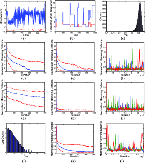
Figure 6: (a) Observation sequence (blue) and true state sequence (red) for a three-state HMM with state persistence. (b) Example of the sticky HDP-HMM direct assignment Gibbs sampler splitting temporally separated examples of the same true state (red) into multiple estimated states (blue) at Gibbs iteration 1000. (c) Histogram of the inferred self-transition proportion parameter, $\rho$, for the sticky HDP-HMM blocked sampler. For the original HDP-HMM, the median (solid blue) and 10th and 90th quantiles (dashed red) of Hamming distance between the true and estimated state sequences over the first 1000 Gibbs samples from 200 chains are shown for the (d) direct assignment sampler, and (e) blocked sampler. (f) Hamming distance over 30,000 Gibbs samples from three chains of the original HDP-HMM blocked sampler. (g)–(i) Analogous plots to (d) and (f) for the sticky HDP-HMM. (k) and (l) Plots analogous to (e) and (f) for a nonsticky HDP-HMM using beam sampling. (j) A histogram of the effective beam sampler truncation level, $L_{\mathrm{eff}}$, over the 30,000 Gibbs iterations from the three chains (blue) compared to the fixed truncation level, $L=20$, used in the truncated sticky HDP-HMM blocked sampler results (red).

We thus propose using a variant of the HMM forward–backward procedure [Rabiner (1989)] to harness the Markovian structure and jointly sample the state sequence $z_{1:T}$ given the observations $y_{1:T}$, transition probabilities $\pi_{k}$, and parameters $\theta_{k}$. There are two main mechanisms for sampling in an uncollapsed HDP model (i.e., one that instantiates the parameters $\pi_{k}$ and $\theta_{k}$): one is to employ slice sampling while the other is to consider a truncated approximation to the HDP. For the HDP-HMM, a slice sampler, referred to as beam sampling, was recently developed [Van Gael et al. (2008)]. This sampler harnesses the efficiencies of the forward–backward algorithm without having to fix a truncation level for the HDP. However, as we elaborate upon in Section 6.1, this sampler suffers from slower mixing rates than the block sampler we propose, which utilizes a fixed-order truncation of the HDP-HMM. Although a fixed truncation reduces our model to a parametric Bayesian HMM, the specific hierarchical prior induced by a truncation of the fully nonparametric HDP significantly improves upon classical parametric Bayesian HMMs. Specifically, a fixed degree $L$ truncation encourages each transition distribution to be sparse over the set of $L$ possible HMM states, and simultaneously encourages transitions from different states to have similar sparsity structures. That is, the truncated HDP prior leads to a shared sparse subset of the $L$ possible states. See Section 6.3 for a comparison with standard parametric modeling.

There are multiple methods of approximating the countably infinite transition distributions via truncations. One approach is to terminate the stick-breaking construction after some portion of the stick has already been broken and assign the remaining weight to a single component. This approximation is referred to as the truncated Dirichlet process. Another method is to consider the degree $L$ weak limit approximation to the DP [Ishwaran and Zarepour (2002c)],

$$\operatorname{GEM}_{L}(\alpha)\triangleq\operatorname{Dir}(\alpha/L,\dots,\alpha/L),$$ (14)

where $L$ is a number that exceeds the total number of expected HMM states. Both of these approximations, which are presented in Ishwaran and Zarepour (2000a, 2002c), encourage the learning of models with fewer than $L$ components while allowing the generation of new components, upper bounded by $L$, as new data are observed. We choose to use the second approximation because of its simplicity and computational efficiency. The two choices of approximations are compared in Kurihara, Welling and Teh (2007), and little to no practical differences are found. Using a weak limit approximation to the Dirichlet process prior on $\beta$ (i.e., employing a finite Dirichlet prior) induces a finite Dirichlet prior on $\pi_{j}$:

$$\beta|\gamma \sim \operatorname{Dir}(\gamma/L,\dots,\gamma/L),$$ (15)

$$\pi_{j}|\alpha,\beta \sim \operatorname{Dir}(\alpha\beta_{1},\dots,\alpha\beta_{L}).$$ (16)

As $L\rightarrow\infty$, this model converges in distribution to the HDP mixture model [Teh et al. (2006)].

The Gibbs sampler using blocked resampling of $z_{1:T}$ is derived in the Supplementary Material [Fox et al. (2010)]; an outline of the resulting algorithm is also presented (see Algorithm 3). A similar sampler has been used for inference in HDP hidden Markov trees [Kivinen, Sudderth and Jordan (2007)]. However, this work did not consider the complications introduced by multimodal emissions, which we explore in Section 7.

The blocked sampler is initialized by drawing $L$ parameters $\theta_{k}$ from the base measure, $\beta$ from its $L$-dimensional symmetric Dirichlet prior, and the $L$ transition distributions $\pi_{k}$ from the induced $L$-dimensional Dirichlet prior specified in equation (15). The hyperparameters are also drawn from the prior. Based on the sampled parameters and transition distributions, one can block sample $z_{1:T}$ and proceed as in Algorithm 3 of the Supplementary Material [Fox et al. (2010)].

5.3 Hyperparameters

We treat the hyperparameters in the sticky HDP-HMM as unknown quantities and perform full Bayesian inference over these quantities. This emphasizes the role of the data in determining the number of occupied states and the degree of self-transition bias. Our derivation of sampling updates for the hyperparameters of the sticky HDP-HMM is presented in the Supplementary Material [Fox et al. (2010)]; it roughly follows that of the original HDP-HMM [Teh et al. (2006)]. A key step which simplifies our inference procedure is to note that since we have the deterministic relationships

$$\alpha = (1-\rho)(\alpha+\kappa),$$

$$\kappa = \rho(\alpha+\kappa),\vspace*{-2pt}$$

we can treat $\rho$ and $\alpha+\kappa$ as our hyperparameters and sample these values instead of sampling $\alpha$ and $\kappa$ directly.

6 Experiments with synthetic data

In this section we explore the performance of the sticky HDP-HMM relative to the original model (i.e., the model with $\kappa=0$) in a series of experiments with synthetic data. We judge performance according to two metrics: our ability to accurately segment the data according to the underlying state sequence, and the predictive likelihood of held-out data under the inferred model. We additionally assess the improvements in mixing rate achieved by using the blocked sampler of Section 5.2.

6.1 Gaussian emissions

We begin our analysis of the sticky HDP-HMM performance by examining a set of simulated data generated from an HMM with Gaussian emissions. The first data set is generated from an HMM with a high probability of self-transition. Here, we aim to show that the original HDP-HMM inadequately captures state persistence. The second data set is from an HMM with a high probability of leaving the current state. In this scenario, our goal is to demonstrate that the sticky HDP-HMM is still able to capture rapid dynamics by inferring a small probability of self-transition.

For all of the experiments with simulated data, we used weakly informative hyperpriors. We placed a $\operatorname{Gamma}(1,0.01)$ prior on the concentration parameters $\gamma$ and $(\alpha+\kappa)$. The self-transition proportion parameter $\rho$ was given a $\operatorname{Beta}(10,1)$ prior. The parameters of the base measure were set from the data, as will be described for each scenario.

State persistence

The data for the high persistence case were generated from a three-state HMM with a 0.98 probability of self-transition and equal probability of transitions to the other two states. The observation and true state sequences for the state persistence scenario are shown in Figure 6(a). We placed a normal inverse-Wishart prior on the space of mean and variance parameters and set the hyperparameters as follows: 0.01 pseudocounts, mean equal to the empirical mean, three degrees of freedom, and scale matrix equal to 0.75 times the empirical variance. We used this conjugate base measure so that we may directly compare the performance of the blocked and direct assignment samplers. For the blocked sampler, we used a truncation level of $L=20$.

In Figure 6(d)–(h), we plot the $10$th, $50$th and $90$th quantiles of the Hamming distance between the true and estimated state sequences over the 1000 Gibbs iterations using the direct assignment and blocked samplers on the sticky and original HDP-HMM models. To calculate the Hamming distance, we used the Munkres algorithm [Munkres (1957)] to map the randomly chosen indices of the estimated state sequence to the set of indices that maximize the overlap with the true sequence.

From these plots, we see that the burn-in rate of the blocked sampler using the sticky HDP-HMM is significantly faster than that of any other sampler-model combination. As expected, the sticky HDP-HMM with the sequential, direct assignment sampler gets stuck in state sequence assignments from which it is hard to move away, as conveyed by the flatness of the Hamming error versus iteration number plot in Figure 6(g). For example, the estimated state sequence of Figure 6(b) might have similar parameters associated with states 3, 7, 10 and 11 so that the likelihood is in essence the same as if these states were grouped, but this sequence has a large error in terms of Hamming distance and it would take many iterations to move away from this assignment. Incorporating the blocked sampler with the original HDP-HMM improves the Hamming distance performance relative to the sequential, direct assignment sampler for both the original and sticky HDP-HMM; however, the burn-in rate is still substantially slower than that of the blocked sampler on the sticky model.

As discussed earlier, a beam sampling algorithm [Van Gael et al. (2008)] has been proposed which adapts slice sampling methods [Robert (2007)] to the HDP-HMM. This approach uses a set of auxiliary slice variables, one for each observation, to effectively truncate the number of state transitions that must be considered at every Gibbs sampling iteration. Dynamic programming methods can then be used to jointly resample state assignments. The beam sampler was inspired by a related approach for DP mixture models [Walker (2007)], which is conceptually similar to retrospective sampling methods [Papaspiliopoulos and Roberts (2008)]. In comparison to our fixed-order, weak-limit truncation of the HDP-HMM, the beam sampler provides an asymptotically exact algorithm. However, the beam sampler can be slow to mix relative to our blocked sampler on the fixed, truncated model (see Figure 6 for an example comparison). The issue is that in order to consider a transition which has low prior probability, one needs a correspondingly rare slice variable sample at that time. Thus, even if the likelihood cues are strong, to be able to consider state sequences with several low-prior-probability transitions, one needs to wait for several rare events to occur when drawing slice variables. By considering the full, exponentially large set of paths in the truncated state space, we avoid this problem. Of course, the trade-off between the computational cost of the blocked sampler on the fixed, truncated model ($O(TL^{2})$) and the slower mixing rate of the beam sampler yields an application-dependent sampler choice.

The Hamming distance plots of Figure 6(k) and (l), when compared to those of Figure 6(e) and (f), depict the substantially slower mixing rate of the beam sampler compared to the blocked sampler (both using a nonsticky HDP-HMM). However, the theoretical computational benefit of the beam sampler can be seen in Figure 6(j). In this plot, we present a histogram of the effective truncation level, $L_{\mathrm{eff}}$, used over the 30,000 Gibbs iterations on three chains. We computed this effective truncation level by summing over the number of state transitions considered during a full sweep of sampling $z_{1:T}$ and then dividing this number by the length of the data set, $T$, and taking the square root. Finally, on a more technical note, our fixed, truncated model allows for more vectorization of the code than the beam sampler. Thus, in practice, the difference in computation time between the samplers is significantly less than the $O(L^{2}/L^{2}_{\mathrm{eff}})$ factor obtained by counting state transitions.

From this point onward, we present results only from blocked sampling since we have seen the clear advantages of this method over the sequential, direct assignment sampler.

Fast state-switching

In order to warrant the general use of the sticky model, one would like to know that the sticky parameter incorporated in the model does not preclude learning models with fast dynamics. To this end, we explored the performance of the sticky HDP-HMM on data generated from a model with a high probability of switching between states. Specifically, we generated observations from a four-state HMM with the following transition probability matrix:

$$\left[\matrix{0.4&0.4&0.1&0.1\cr 0.4&0.4&0.1&0.1\cr 0.1&0.1&0.4&0.4\cr 0.1&0.1&0.4&0.4}\right].$$ (18)

We once again used a truncation level $L=20$. Since we are restricting ourselves to the blocked Gibbs sampler, it is no longer necessary to use a conjugate base measure. Instead we placed an independent Gaussian prior on the mean parameter and an inverse-Wishart prior on the variance parameter. For the Gaussian prior, we set the mean and variance hyperparameters to be equal to the empirical mean and variance of the entire data set. The inverse-Wishart hyperparameters were set such that the expected variance is equal to 0.75 times that of the entire data set, with three degrees of freedom.

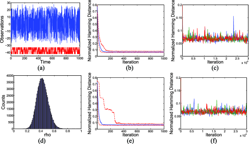
Figure 7: (a) Observation sequence (blue) and true state sequence (red) for a four-state HMM with fast state switching. For the original HDP-HMM using a blocked Gibbs sampler: (b) the median (solid blue) and 10th and 90th quantiles (dashed red) of Hamming distance between the true and estimated state sequences over the first 1000 Gibbs samples from 200 chains, and (c) Hamming distance over 30,000 Gibbs samples from three chains. (d) Histogram of the inferred self-transition parameter, $\rho$, for the sticky HDP-HMM blocked sampler. (e) and (f) Analogous plots to (b) and (c) for the sticky HDP-HMM.

The results depicted in Figure 7 confirm that by inferring a small probability of self-transition, the sticky HDP-HMM is indeed able to capture fast HMM dynamics, and just as quickly as the original HDP-HMM (although with higher variability). Specifically, we see that the histogram of the self-transition proportion parameter $\rho$ for this data set [see Figure 7(d)] is centered around a value close to the true probability of self-transition, which is substantially lower than the mean value of this parameter on the data with high persistence [Figure 6(c)].

6.2 Multinomial emissions

The difference in modeling power, rather than simply burn-in rate, between the sticky and original HDP-HMM is more pronounced when we consider multinomial emissions. This is because the multinomial observations are embedded in a discrete topological space in which there is no concept of similarity between nonidentical observation values. In contrast, Gaussian emissions have a continuous range of values in $\mathbb{R}^{n}$ with a clear notion of closeness between observations under the Lebesgue measure, aiding in grouping observations under a single HMM state’s Gaussian emission distribution, even in the absence of a self-transition bias.

To demonstrate the increased posterior uncertainty with discrete observations, we generated data from a five-state HMM with multinomial emissions with a 0.98 probability of self-transition and equal probability of transitions to the other four states. The vocabulary, or range of possible observation values, was set to 20. The observation and true state sequences are shown in Figure 8(a). We placed a symmetric Dirichlet prior on the parameters of the multinomial distribution, with the Dirichlet hyperparameters equal to 2 [i.e., $\operatorname{Dir}(2,\dots,2)]$.

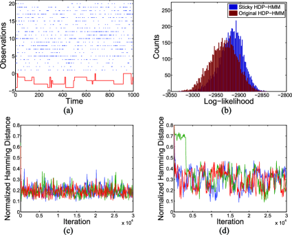
Figure 8: (a) Observation sequence (blue) and true state sequence (red) for a five-state HMM with multinomial observations. (b) Histogram of the predictive probability of test sequences using the inferred parameters sampled every 100th iteration from Gibbs iterations 10,000–30,000 for the sticky and original HDP-HMM. The Hamming distances over 30,000 Gibbs samples from three chains are shown for the (c) sticky HDP-HMM and (d) original HDP-HMM.

From Figure 8, we see that even after burn-in, many fast-switching state sequences have significant posterior probability under the nonsticky model, leading to sweeps through regions of larger Hamming distance error. A qualitative plot of one such inferred sequence after 30,000 Gibbs iterations is shown in Figure 1(c). Such sequences have negligible posterior probability under the sticky HDP-HMM formulation.

In some applications, such as the speaker diarization problem that is explored in Section 8, one cares about the inferred segmentation of the data into a set of state labels. In this case, the advantage of incorporating the sticky parameter is clear. However, it is often the case that the metric of interest is the predictive power of the fitted model, not the accuracy of the inferred state sequence. To study performance under this metric, we simulated 10 test sequences using the same parameters that generated the training sequence. We then computed the likelihood of each of the test sequences under the set of parameters inferred at every $100$th Gibbs iteration from iterations 10,000–30,000. This likelihood was computed by running the forward–backward algorithm of Rabiner (1989). We plot these results as a histogram in Figure 8(b). From this plot, we see that the fragmentation of data into redundant HMM states can also degrade the predictive performance of the inferred model. Thus, the sticky parameter plays an important role in the Bayesian nonparametric learning of HMMs even in terms of model averaging.

6.3 Comparison to independent sparse Dirichlet prior

We have alluded to the fact that the shared sparsity of the HDP-HMM induced by $\beta$ is essential for inferring sparse representations of the data. Although this is clear from the perspective of the prior model, or, equivalently, the generative process, it is not immediately obvious how much this hierarchical Bayesian constraint helps us in posterior inference. Once we are in the realm of considering a fixed, truncated approximation to the HDP-HMM, one might propose an alternate model in which we simply place a sparse Dirichlet prior, $\operatorname{Dir}(\alpha/L,\dots,\alpha/L)$ with $\alpha/L<1$, independently on each row of the transition matrix. This is equivalent to setting $\beta=[1/L,\dots,1/L]$ in the truncated HDP-HMM, which can also be achieved by letting the hyperparameter $\gamma$ tend to infinity. Indeed, when the data do not exhibit shared sparsity or when the likelihood cues are sufficiently strong, the independent sparse Dirichlet prior model can perform as well as the truncated HDP-HMM. However, in scenarios such as the one depicted in Figure 9, we see substantial differences in performance by considering the HDP-HMM, as well as the inclusion of the sticky parameter. We explored the relative performance of the HDP-HMM and sparse Dirichlet prior model, with and without the sticky parameter, on such a Markov model with multinomial emissions on a vocabulary of size 20. We placed a $\operatorname{Dir}(0.1,\dots,0.1)$ prior on the parameters of the multinomial distribution. For the sparse Dirichlet prior model, we assumed a state space of size 50, which is the same as the truncation level we chose for the HDP-HMM (i.e., $L=50$). The results are presented in Figure 10. From these plots, we see that the hierarchical Bayesian approach of the HDP-HMM does, in fact, improve the fitting of a model with shared sparsity. The HDP-HMM consistently infers fewer HMM states and more representative model parameters. As a result, the HDP-HMM has higher predictive likelihood on test data, with an additional benefit gained from using the sticky parameter.

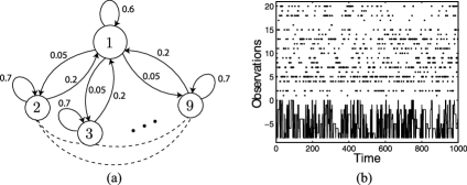
Figure 9: (a) State transition diagram for a nine-state HMM with one main state (labeled 1) and eight sub-states (labeled 2–9). All states have a significant probability of self-transition. From the main state, all other states are equally likely. From a sub-state, the most likely nonself-transition is a transition back to the main state. However, all sub-states have a small probability of transitioning to another sub-state, as indicated by the dashed arcs. (b) Observation sequence (top) and true state sequence (bottom) generated by the nine-state HMM with multinomial observations.

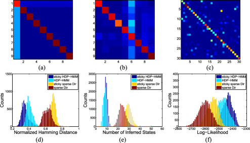
Figure 10: (a) The true transition probability matrix (TPM) associated with the state transition diagram of Figures 9. (b) and (c) The inferred TPM at the 30,000th Gibbs iteration for the sticky HDP-HMM and sticky sparse Dirichlet model, respectively, only examining those states with more than 1% of the assignments. For the HDP-HMM and sparse Dirichlet model, with and without the sticky parameter, we plot: (d) the Hamming distance error over 10,000 Gibbs iterations, (e) the inferred number of states with more than 1% of the assignments, and (f) the predictive probability of test sequences using the inferred parameters sampled every 100th iteration from Gibbs iterations 5000–10,000.

Note that the results of Figure 10(f) also motivate the use of the sticky parameter in the more classical setting of a finite HMM with a standard Dirichlet sparsity prior. A motivating example of the use of sparse Dirichlet priors for finite HMMs is presented in Johnson (2007).

7 Multimodal emission densities

In many application domains, the data associated with each hidden state may have a complex, multimodal distribution. We propose to model such emission distributions nonparametrically, using a DP mixture of Gaussians. This formulation is related to the nested DP [Rodriguez, Dunson and Gelfand (2008)], which uses a Dirichlet process to partition data into groups, and then models each group via a Dirichlet process mixture. The bias toward self-transitions allows us to distinguish between the underlying HDP-HMM states. If the model were free to both rapidly switch between HDP-HMM states and associate multiple Gaussians per state, there would be considerable posterior uncertainty. Thus, it is only with the sticky HDP-HMM that we can effectively fit such models.

We augment the HDP-HMM state $z_{t}$ with a term $s_{t}$ indexing the mixture component of the $z_{t}$th emission density. For each HDP-HMM state, there is a unique stick-breaking measure $\psi_{k}\sim\operatorname{GEM}(\sigma)$ defining the mixture weights of the $k$th emission density so that $s_{t}\sim\psi_{z_{t}}$. Given the augmented state $(z_{t},s_{t})$, the observation $y_{t}$ is generated by the Gaussian component with parameter $\theta_{z_{t},s_{t}}$. Note that both the HDP-HMM state index and mixture component index are allowed to take values in a countably infinite set. See Figure 5(b).

7.1 Direct assignment sampler

Many of the steps of the direct assignment sampler for the sticky HDP-HMM with DP emissions remain the same as for the regular sticky HDP-HMM. Specifically, the sampling of the global transition distribution $\beta$, the table counts $m_{jk}$ and $\bar{m}_{jk}$, and the override variables $w_{jt}$ are unchanged. The difference arises in how we sample the augmented state $(z_{t},s_{t})$.

The joint distribution on the augmented state, having marginalized the transition distributions $\pi_{k}$ and emission mixture weights $\psi_{k}$, is given by

$$p(z_{t}=k,s_{t}=j|z_{\backslash t},s_{\backslash t},y_{1:T},\beta,\alpha,\sigma,\kappa,\lambda)$$

$$\qquad=p(s_{t}=j|z_{t}=k,z_{\backslash t},s_{\backslash t},y_{1:T},\sigma,\lambda),$$

$$\hskip 20.0ptp(z_{t}=k|z_{\backslash t},s_{\backslash t},y_{1:T},\beta,\alpha,\kappa,\lambda).$$

We then block-sample $(z_{t},s_{t})$ by first sampling $z_{t}$, followed by $s_{t}$ conditioned on the sampled value of $z_{t}$. The term $p(s_{t}=j|z_{t}=k,z_{\backslash t},s_{\backslash t},y_{1:T},\sigma,\lambda)$ relies on how many observations are currently assigned to the $j$th mixture component of state $k$. These conditional distributions are derived in the Supplementary Material [Fox et al. (2010)], which also contains an outline of the resulting Gibbs sampler in Algorithm 2.

7.2 Blocked sampler

To implement blocked resampling of $(z_{1:T},s_{1:T})$, we use weak limit approximations to both the HDP-HMM and DP emissions, approximated to levels $L$ and $L^{\prime}$, respectively. The posterior distributions for $\beta$ and $\pi_{k}$ remain unchanged from the sticky HDP-HMM; that of $\psi_{k}$ is given by

$$\psi_{k}|z_{1:T},s_{1:T},\sigma\sim\operatorname{Dir}(\sigma/L^{\prime}+n^{\prime}_{k1},\dots,\sigma/L^{\prime}+n^{\prime}_{kL^{\prime}}),$$ (19)

where $n^{\prime}_{k\ell}$ is the number of $s_{t}$ taking a value $\ell$ when $z_{t}=k$. (i.e., the number of observations assigned to the $k$th state’s $\ell$th mixture component). The procedure for sampling the augmented state $(z_{1:T},s_{1:T})$ is derived in the Supplementary Material [see Algorithm 4, Fox et al. (2010)].

7.3 Assessing the multimodal emissions model

In this section we evaluate the ability of the sticky HDP-HMM to infer multimodal emission distributions relative to the model without the sticky parameter. We generated data from a five-state HMM with mixture-of-Gaussian emissions, where the number of mixture components for each emission distribution was chosen randomly from a uniform distribution on $\{1,2,\ldots,10\}$. Each component of the mixture was equally weighted and the probability of self-transition was set to 0.98, with equal probabilities of transitions to the other states. The large probability of self-transition is what disambiguates this process from one with many more HMM states, each with a single Gaussian emission distribution. The resulting observation and true state sequences are shown in Figure 11(a).

We once again used a nonconjugate base measure and placed a Gaussian prior on the mean parameter and an independent inverse-Wishart prior on the variance parameter of each Gaussian mixture component. The hyperparameters for these distributions were set from the data in the same manner as in the fast-switching scenario. Consistent with the sticky HDP-HMM concentration parameters $\gamma$ and $(\alpha+\kappa)$, we placed a weakly informative $\operatorname{Gamma}(1,0.01)$ prior on the concentration parameter $\sigma$ of the DP emissions. All results are for the blocked sampler with truncation levels $L=L^{\prime}=20$.

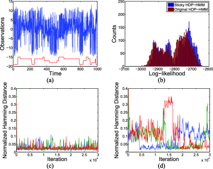
Figure 11: (a) Observation sequence (blue) and true state sequence (red) for a five-state HMM with mixture-of-Gaussian observations. (b) Histogram of the predictive probability of test sequences using the inferred parameters sampled every 100th iteration from Gibbs iterations 10,000–30,000 for the sticky and original HDP-HMM. The Hamming distance over 30,000 Gibbs samples from three chains are shown for the (c) sticky HDP-HMM and (d) original HDP-HMM, both with DP emissions.

In Figure 11 we compare the performance of the sticky HDP-HMM with DP emissions to that of the original HDP-HMM with DP emissions (i.e., DP emissions, but no bias toward self-transitions). As with the multinomial observations, when the distance between observations does not directly factor into the grouping of observations into HMM states, there is a considerable amount of posterior uncertainty in the underlying HMM state of the nonsticky model. Even after 30,000 Gibbs samples, there are still state sequence sample paths with very rapid dynamics. The result of this fragmentation into redundant states is a slight reduction in predictive performance on test sequences, as in the multinomial emission case. See Figure 11(b).

8 Speaker diarization results

Recall the speaker diarization task from Section 2, which involves segmenting audio recordings from the NIST Rich Transcription 2004–2007 database into speaker-homogeneous regions while simultaneously identifying the number of speakers. In this section we present our results on applying the sticky HDP-HMM with DP emissions to the speaker diarization task.

A minimum speaker duration of 500 ms was set by associating two preprocessed MFCCs with each hidden state. We also tied the covariances of within-state mixture components (i.e., each speaker-specific mixture component was forced to have identical covariance structure), and used a nonconjugate prior on the mean and covariance parameters. We placed a normal prior on the mean parameter with mean equal to the empirical mean and covariance equal to 0.75 times the empirical covariance, and an inverse-Wishart prior on the covariance parameter with 1000 degrees of freedom and expected covariance equal to the empirical covariance. Our choice of a large degrees of freedom is akin to an empirical Bayes approach in that it concentrates the mass of the prior in reasonable regions based on the data. Such an approach is often helpful in high-dimensional applied problems since our sampler relies on forming new states (i.e., speakers) based on parameters drawn from the prior. Issues of exploration in this high-dimensional space increase the importance of the setting of the base measure. For the concentration parameters, we placed a $\operatorname{Gamma}(12,2)$ prior on $\gamma$, a $\operatorname{Gamma}(6,1)$ prior on $\alpha+\kappa$, and a $\operatorname{Gamma}(1,0.5)$ prior on $\sigma$. The self-transition parameter $\rho$ was given a $\operatorname{Beta}(500,5)$ prior. For each of the 21 meetings, we ran 10 chains of the blocked Gibbs sampler for 10,000 iterations for both the original and sticky HDP-HMM with DP emissions. We used a sticky HDP-HMM truncation level of $L=15$, where the DP-mixture-of-Gaussians emission distribution associated with each of these $L$ HMM states was truncated to $L^{\prime}=30$ components. Our choice of $L$ significantly exceeds the typical number of speakers, which in the NIST database tends to be between 4 and 6. In practice, our sampler never approached using the full set of possible states and emission components.

In order to explore the importance of capturing the temporal dynamics, we also compare our sticky HDP-HMM performance to that of a Dirichlet process mixture of Gaussians that simply pools together the data from each meeting, ignoring the time indices associated with the observations. We considered a truncated Dirichlet process mixture model with $L=50$ components and a $\operatorname{Gamma}(6,1)$ prior on the concentration parameter $\gamma$. The base measure was set as in the sticky HDP-HMM.

For the NIST speaker diarization evaluations, the goal is to produce a single segmentation for each meeting. Due to the label-switching issue (i.e., under our exchangeable prior, labels are arbitrary entities that do not necessarily remain consistent over Gibbs iterations), we cannot simply integrate over multiple Gibbs-sampled state sequences. We propose two solutions to this problem. The first, which we refer to as the likelihood metric, is to simply choose from a fixed set of Gibbs samples the one that produces the largest likelihood given the estimated parameters (marginalizing over state sequences), and then produce the corresponding Viterbi state sequence. This heuristic, however, is sensitive to overfitting and will, in general, be biased toward solutions with more states.

An alternative, and more robust, metric is what we refer to as the minimum expected Hamming distance. We first choose a large reference set $\mathcal{R}$ of state sequences produced by the Gibbs sampler and a possibly smaller set of test sequences $\mathcal{T}$. Then, for each sequence $z^{(i)}$ in the test set $\mathcal{T}$, we compute the empirical mean Hamming distance between the test sequence and the sequences in the reference set $\mathcal{R}$; we denote this empirical mean by $\hat{H}_{i}$. We then choose the test sequence $z^{(j^{*})}$ that minimizes this expected Hamming distance. That is,

$$z^{(j^{*})}=\arg\min_{z^{(i)}\in\mathcal{T}}\hat{H}_{i}.$$

The empirical mean Hamming distance $\hat{H}_{i}$ is a label-invariant loss function since it does not rely on labels remaining consistent across samples—we simply compute

$$\hat{H}_{i}=\frac{1}{|\mathcal{R}|}\sum_{z^{(j)}\in\mathcal{R}}\operatorname{Hamm}\bigl{(}z^{(i)},z^{(j)}\bigr{)},$$

where $\operatorname{Hamm}(z^{(i)},z^{(j)})$ is the Hamming distance between sequences $z^{(i)}$ and $z^{(j)}$ after finding the optimal permutation of the labels in test sequence $z^{(i)}$ to those in reference sequence $z^{(j)}$. At a high level, this method for choosing state sequence samples aims to produce segmentations of the data that are typical samples from the posterior. Jasra, Holmes and Stephens (2005) provide an overview of some related techniques to address the label-switching issue. Although we could have chosen any label-invariant loss function to minimize, we chose the Hamming distance metric because it is closely related to the official NIST diarization error rate (DER) that is calculated during the evaluations. The final metric by which the speaker diarization algorithms are judged is the overall DER, a weighted average over the set of meetings based on the length of each meeting.

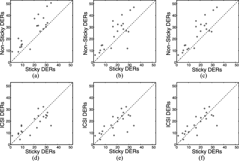
Figure 12: (a)–(c) For each of the 21 meetings, comparison of diarizations using sticky vs. original HDP-HMM with DP emissions. In (a) we plot the DERs corresponding to the Viterbi state sequence using the parameters inferred at Gibbs iteration 10,000 that maximize the likelihood, and in (b) the DERs using the state sequences that minimize the expected Hamming distance. Plot (c) is the same as (b), except for running the 10 chains for meeting 16 out to 50,000 iterations. (d)–(f) Comparison of the sticky HDP-HMM with DP emissions to the ICSI errors under the same conditions.

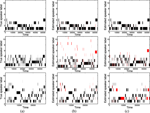
Figure 13: Qualitative results for meetings AMI_20041210-1052 (meeting 1, top), CMU_20050228-1615 (meeting 3, middle) and NIST_20051102-1323 meeting (meeting 16, bottom). (a) True state sequence with the post-processed regions of overlapping- and nonspeech time steps removed. (b) and (c) Plotted only over the time-steps as in (a), the state sequences inferred by the sticky HDP-HMM with DP emissions at Gibbs iteration 10,000 chosen using the most likely and minimum expected Hamming distance metrics, respectively. Incorrect labels are shown in red. For meeting 1, the maximum likelihood and minimum expected Hamming distance diarizations are similar, whereas in meeting 3 we clearly see the sensitivity of the maximum likelihood metric to overfitting. The minimum expected Hamming distance diarization for meeting 16 has more errors than that of the maximum likelihood due to poor mixing rates and many samples failing to identify a speaker.

In Figure 12(a) we report the DER of the chain with the largest likelihood given the parameters estimated at the 10,000th Gibbs iteration for each of the 21 meetings, comparing the sticky and original HDP-HMM with DP emissions. We see that the sticky model’s temporal smoothing provides substantial performance gains. Although not depicted in this paper, the likelihoods based on the parameter estimates under the original HDP-HMM are almost always higher than those under the sticky model. This phenomenon is due to the fact that without the sticky parameter, the HDP-HMM over-segments the data and thus produces parameter estimates more finely tuned to the data, resulting in higher likelihoods. Since the original HDP-HMM is contained within the class of sticky models (i.e., when $\kappa=0$), there is some probability that state sequences similar to those under the original model will eventually arise using the sticky model. Thus, since the parameters associated with these fast-switching sequences result in higher likelihood of the data, the likelihood metric is not very robust—one would expect the performance under the sticky model to degrade given enough Gibbs chains and/or iterations. In Figure 12(b) we instead report the DER of the chain whose state sequence estimate at Gibbs iteration 10,000 (this defines the test set $\mathcal{T}$) minimizes the expected Hamming distance to the sequences estimated every 100 Gibbs iteration, discarding the first 5000 iterations (this defines the reference set $\mathcal{R}$). Due to the slow mixing rate of the chains in this application, we additionally discard samples whose normalized log-likelihood is below 0.1 units of the maximum at Gibbs iteration 10,000. From this figure, we see that the sticky model still significantly outperforms the original HDP-HMM, implying that most state sequences produced by the original model are worse, not just the one corresponding to the most likely sample. Example maximum likelihood and minimum expected Hamming distance diarizations are displayed in Figure 13. One noticeable exception to this trend is the NIST_20051102-1323 meeting (meeting 16). For the sticky model, the state sequence using the maximum likelihood metric had very low DER [see Figure 13(b)]; however, there were many chains that merged speakers and produced segmentations similar to the one in Figure 13(c), resulting in such a sequence minimizing the expected Hamming distance. See Section 9 for a discussion on the issue of merged speakers. Running meeting 16 for 50,000 Gibbs iterations improved the performance, as depicted by the revised results in Figure 12(c). We summarize our overall performance in Table 1, and note that (when using the 50,000 Gibbs iterations for meeting 16 and 10,000 Gibbs iterations for all other meetings) we obtain an overall DER of 17.84% using the sticky HDP-HMM versus the 23.91% of the original HDP-HMM model. Alternatively, when constrained to single Gaussian emissions the sticky HDP-HMM and original HDP-HMM have overall DERs of 34.97% and 36.89%, respectively, which clearly demonstrates the importance of considering DP emissions. When considering the DP mixture-of-Gaussians model (ignoring the time indices associated with the observations), the overall DER is 72.67%. If one uses the ground truth labels to map multiple inferred DP mixture components to a single speaker label, the overall DER drops to 54.19%. The poor performance of the DP mixture-of-Gaussians model, even when assuming that ground truth labels are available, which would not be the case in practice, illustrates the importance of the temporal dynamics captured by the HMM.

Table 1: Overall DERs for the sticky and original HDP-HMM with DP emissions using the minimum expected Hamming distance and maximum likelihood metrics for choosing state sequences at Gibbs iteration 10,000

Overall DERs (%)	Min Hamming	Max likelihood	2-Best	5-Best
Sticky HDP-HMM	19.01 (17.84)	19.37	16.97	14.61
Nonsticky HDP-HMM	23.91 (17.84)	25.91	23.67	21.06

[]Notes: For the maximum likelihood criterion, we show the best overall DER if we consider the top two or top five most likely candidates. The number in the parentheses is the performance when running meeting 16 for 50,000 Gibbs iterations. The overall ICSI DER is 18.37%, while the best achievable DER with the chosen acoustic preprocessing is 10.57%.

As a further comparison, the algorithm that was by far the best performer at the 2007 NIST competition—the algorithm developed by a team at the International Computer Science Institute (ICSI) [Wooters and Huijbregts (2007)]—has an overall DER of 18.37%. The ICSI team’s algorithm uses agglomerative clustering, and requires significant tuning of parameters on representative training data. In contrast, our hyperparameters are automatically set meeting-by-meeting, as outlined at the beginning of this section. An additional benefit of the sticky HDP-HMM over the ICSI approach is the fact that there is inherent posterior uncertainty in this task, and by taking a Bayesian approach, we are able to provide several interpretations. Indeed, when considering the best per-meeting DER for the five most likely samples, our overall DER drops to 14.61% (see Table 1). Although not helpful in the NIST evaluations, which require a single segmentation, providing multiple segmentations could be useful in practice.

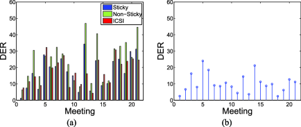
Figure 14: (a) Chart comparing the DERs of the sticky and original HDP-HMM with DP emissions to those of ICSI for each of the 21 meetings. Here, we chose the state sequence at the 10,000th Gibbs iteration that minimizes the expected Hamming distance. For meeting 16 using the sticky HDP-HMM with DP emissions, we chose between state sequences at Gibbs iteration 50,000. (b) DERs associated with using ground truth speaker labels for the post-processed data. Here, we assign undetected nonspeech a label different than the preprocessed nonspeech.

To ensure a fair comparison, we use the same speech/nonspeech preprocessing and acoustic features as ICSI, so that the differences in our performance are due to changes in the identified speakers. As depicted in Figure 14, both our performance and that of ICSI depend significantly on the quality of this preprocessing step. For the periods of nonspeech that are incorrectly identified as speech during preprocessing, we are forced to produce errors on these sections since they will be assigned an HMM label (and thus a speaker label) that is separate from the label assigned to the preprocessed sections labeled as nonspeech. Another source of errors are periods of overlapping speech, which impede our ability to clearly identify a single speaker. In Figure 14(a) we compare the meeting-by-meeting DERs of the sticky HDP-HMM, the original HDP-HMM, and the ICSI algorithm. If we use the ground truth speaker labels for the post-processed data (assigning undetected nonspeech a label different than the preprocessed nonspeech), the resulting overall DER is 10.57% with meeting-by-meeting DERs displayed in Figure 14(b). This number provides a lower bound on the achievable performance using the speech/nonspeech preprocessing, our block-averaging of features, and our assumptions of minimum duration. Beyond these forced errors, it is clear from Figure 14(a) that the sticky HDP-HMM with DP emissions provides performance comparable to that of the ICSI algorithm, while the original HDP-HMM with DP emissions performs significantly worse. Overall, the results presented in this section demonstrate that the sticky HDP-HMM with DP emissions provides an elegant and empirically effective speaker diarization method.

9 Discussion

We have developed a Bayesian nonparametric approach to the problem of speaker diarization, building on the HDP-HMM presented in Teh et al. (2006). Although the original HDP-HMM does not yield competitive speaker diarization performance due to its inadequate modeling of the temporal persistence of states, the sticky HDP-HMM that we have presented here resolves this problem and yields a state-of-the-art solution to the speaker diarization problem.

We have also shown that this sticky HDP-HMM allows a fully Bayesian nonparametric treatment of multimodal emissions, disambiguated by its bias toward self-transitions. Accommodating multimodal emissions is essential for the speaker diarization problem and is likely to be an important ingredient in other applications of the HDP-HMM to problems in speech technology.

We also presented efficient sampling techniques with mixing rates that improve on the state of the art by harnessing the Markovian structure of the HDP-HMM. Specifically, we proposed employing a truncated approximation to the HDP and block-sampling the state sequence using a variant of the forward–backward algorithm. Although the blocked samplers yield substantially improved mixing rates over the sequential, direct assignment samplers, there are still some pitfalls to these sampling methods. One issue is that for each new considered state, the parameter sampled from the prior distribution must better explain the data than the parameters associated with other states that have already been informed by the data. In high-dimensional applications, and in cases where state-specific emission distributions are not clearly distinguishable, this method for adding new states poses a significant challenge. Indeed, both issues arise in the speaker diarization task and we did have difficulties with mixing. Further evidence of this is presented in the trace plots in Figure 15, where we plot log-likelihoods, Hamming distances and speaker counts for 10,000 Gibbs sampling iterations of meeting 5 and 100,000 iterations of meeting 16. As discussed previously, meeting 16 is the most problematic meeting in our data set, and these plots provide clear evidence that our sampler is not mixing on this meeting. But even on meeting 5, which is more representative of the full set of meetings and which is segmented effectively by our procedure, we see a relatively slow evolution of the sampler, particularly as measured by the number of speakers. Our use of the minimum expected Hamming distance procedure to select samples mitigates this difficulty, but further work on sampling procedures for the sticky HDP-HMM is needed. One possibility is to consider split-merge algorithms similar to those developed in Jain and Neal (2004) for the DP mixture model.

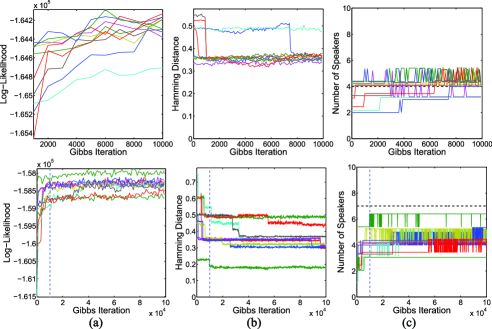
Figure 15: Trace plots of (a) log-likelihood, (b) Hamming distance error and (c) number of speakers for 10 chains for two meetings: CMU_20050912-0900 / meeting 5 (top) and NIST_20051102-1323 / meeting 16 (bottom). For meeting 5, which has behavior representative of the majority of the meetings, we show traces over the 10,000 Gibbs iterations used for the results in Section 8. For meeting 16, we ran the chains out to 100,000 Gibbs iterations to demonstrate the especially slow mixing rate for this meeting. The dashed blue vertical lines indicate 10,000 iterations.

A limitation of the HMM in general is that the observations are assumed conditionally i.i.d. given the state sequence. This assumption is often insufficient in capturing the complex temporal dependencies exhibited in real-world data. Another area of future work is to consider Bayesian nonparametric versions of models better suited to such applications, like the switching linear dynamical system (SLDS) and switching VAR process. A first attempt at developing such models is presented in Fox et al. (2009). An inspiration for the sticky HDP-HMM actually came from considering the original HDP-HMM as a prior for an SLDS. In such scenarios where one does not have direct observations of the underlying state sequence, the issues arising from not properly capturing state persistence are exacerbated. The sticky HDP-HMM presented in this paper provides a robust building block for developing more complex Bayesian nonparametric dynamical models.

References

- Barras et al. (2004) Barras, C., Zhu, X., Meignier, S. and Gauvain, J.-L. (2004). Improving speaker diarization. In Proc. Fall 2004 Rich Transcription Workshop (RT-04), November 2004.
- Beal and Krishnamurthy (2006) Beal, M. J. and Krishnamurthy, P. (2006). Gene expression time course clustering with countably infinite hidden Markov models. In Proc. Conference on Uncertainty in Artificial Intelligence, Cambridge, MA.
- Beal, Ghahramani and Rasmussen (2002) Beal, M. J., Ghahramani, Z. and Rasmussen, C. E. (2002). The infinite hidden Markov model. In Advances in Neural Information Processing Systems 14 577–584. MIT Press, Cambridge, MA.
- Blackwell and MacQueen (1973) Blackwell, D. and MacQueen, J. B. (1973). Ferguson distributions via Pólya urn schemes. Ann. Statist. 1 353–355. \MR0362614
- Chen and Gopalakrishnam (1998) Chen, S. S. and Gopalakrishnam, P. S. (1998). Speaker, environment and channel change detection and clustering via the Bayesian information criterion. In Proc. DARPA Broadcast News Transcription and Understanding Workshop 127–132. Morgan Kaufmann, San Francisco, CA.
- Ferguson (1973) Ferguson, T. S. (1973). A Bayesian analysis of some nonparametric problems. Ann. Statist. 1 209–230. \MR0350949
- Fox et al. (2008) Fox, E. B., Sudderth, E. B., Jordan, M. I. and Willsky, A. S. (2008). An HDP-HMM for systems with state persistence. In Proc. International Conference on Machine Learning, Helsinki, Finland, July 2008.
- Fox et al. (2009) Fox, E. B., Sudderth, E. B., Jordan, M. I. and Willsky, A. S. (2009). Nonparametric Bayesian learning of switching dynamical systems. In Advances in Neural Information Processing Systems 21 457–464.
- Fox et al. (2010) Fox, E. B., Sudderth, E. B., Jordan, M. I. and Willsky, A. S. (2010). Supplement to “A sticky HDP-HMM with application to speaker diarization.” DOI: 10.1214/10-AOAS395SUPP.
- Gales and Young (2007) Gales, M. and Young, S. (2007). The Application of hidden Markov models in speech recognition. Foundations and Trends in Signal Processing 1 195–304.
- Gauvain, Lamel and Adda (1998) Gauvain, J.-L., Lamel, L. and Adda, G. (1998). Partitioning and transcription of broadcast news data. In Proc. International Conference on Spoken Language Processing, Sydney, Australia 1335–1338.
- Hoffman, Cook and Blei (2008) Hoffman, M., Cook, P. and Blei, D. (2008). Data-driven recomposition using the hierarchical Dirichlet process hidden Markov model. In Proc. International Computer Music Conference, Belfast, UK.
- Ishwaran and Zarepour (2000a) Ishwaran, H. and Zarepour, M. (2000a). Markov chain Monte Carlo in approximate Dirichlet and beta two–parameter process hierarchical models. Biometrika 87 371–390. \MR1782485
- Ishwaran and Zarepour (2002b) Ishwaran, H. and Zarepour, M. (2002b). Dirichlet prior sieves in finite normal mixtures. Statist. Sinica 12 941–963. \MR1929973
- Ishwaran and Zarepour (2002c) Ishwaran, H. and Zarepour, M. (2002c). Exact and approximate sum—representations for the Dirichlet process. Canad. J. Statist. 30 269–283. \MR1926065
- Jain and Neal (2004) Jain, S. and Neal, R. M. (2004). A split-merge Markov chain Monte Carlo procedure for the dirichlet process mixture model. J. Comput. Graph. Statist. 13 158–182. \MR2044876
- Jasra, Holmes and Stephens (2005) Jasra, A., Holmes, C. C. and Stephens, D. A. (2005). Markov chain Monte Carlo methods and the label switching problem in Bayesian mixture modeling. Statist. Sci. 20 50–67. \MR2182987
- Johnson (2007) Johnson, M. (2007). Why doesn’t EM find good HMM POS-taggers. In Proc. Joint Conference on Empirical Methods in Natural Language Processing and Computational Natural Language Learning, Prague, Czech Republic.
- Kivinen, Sudderth and Jordan (2007) Kivinen, J. J., Sudderth, E. B. and Jordan, M. I. (2007). Learning multiscale representations of natural scenes using Dirichlet processes. In Proc. International Conference on Computer Vision, Rio de Janeiro, Brazil 1–8.
- Kurihara, Welling and Teh (2007) Kurihara, K., Welling, M. and Teh, Y. W. (2007). Collapsed variational Dirichlet process mixture models. In Proc. International Joint Conferences on Artificial Intelligence, Hyderabad, India.
- Meignier et al. (2000) Meignier, S., Bonastre, J.-F., Fredouille, C. and Merlin, T. (2000). Evolutive HMM for multi-speaker tracking system. In Proc. IEEE International Conference on Acoustics, Speech and Signal Processing (ICASSP), Istanbul, Turkey, June 2000.
- Meignier, Bonastre and Igounet (2001) Meignier, S., Bonastre, J.-F. and Igounet, S. (2001). E-HMM approach for learning and adapting sound models for speaker indexing. In Proc. Odyssey Speaker Language Recognition Workshop, June 2001.
- Munkres (1957) Munkres, J. (1957). Algorithms for the assignment and transportation problems. J. Soc. Industr. Appl. Math. 5 32–38. \MR0093429
- NIST (2007) NIST. Rich transcriptions database. Available at http://www.nist.gov/speech/tests/rt/, 2007.
- Papaspiliopoulos and Roberts (2008) Papaspiliopoulos, O. and Roberts, G. O. (2008). Retrospective Markov chain Monte Carlo methods for Dirichlet process hierarchical models. Biometrika 95 169–186. \MR2409721
- Rabiner (1989) Rabiner, L. R. (1989). A tutorial on hidden Markov models and selected applications in speech recognition. Proc. IEEE 77 257–286.
- Reynolds and Torres-Carrasquillo (2004) Reynolds, D. A. and Torres-Carrasquillo, P. A. (2004). The MIT Lincoln Laboratory RT-04F diarization systems: Applications to broadcast news and telephone conversations. In Proc. Fall 2004 Rich Transcription Workshop (RT-04), November 2004.
- Robert (2007) Robert, C. P. (2007). The Bayesian Choice. Springer, New York.
- Rodriguez, Dunson and Gelfand (2008) Rodriguez, A., Dunson, D. B. and Gelfand, A. E. (2008). The nested Dirichlet process. J. Amer. Statist. Assoc. 103 1131–1154.
- Scott (2002) Scott, S. L. (2002). Bayesian methods for hidden Markov models: Recursive computing in the 21st century. J. Amer. Statist. Assoc. 97 337–351. \MR1963393
- Sethuraman (1994) Sethuraman, J. (1994). A constructive definition of Dirichlet priors. Statist. Sinica 4 639–650. \MR1309433
- Siegler et al. (1997) Siegler, M., Jain, U., Raj, B. and Stern, R. M. (1997). Automatic segmentation, classification and clustering of broadcast news audio. In Proc. DARPA Speech Recognition Workshop 97–99. Morgan Kaufmann, San Francisco, CA.
- Teh et al. (2006) Teh, Y. W., Jordan, M. I., Beal, M. J. and Blei, D. M. (2006). Hierarchical Dirichlet processes. J. Amer. Statist. Assoc. 101 1566–1581. \MR2279480
- Tranter and Reynolds (2006) Tranter, S. E. and Reynolds, D. A. (2006). An overview of automatic speaker diarization systems. IEEE Trans. Audio, Speech Language Process. 14 1557–1565.
- Van Gael et al. (2008) Van Gael, J., Saatci, Y., Teh, Y. W. and Ghahramani, Z. (2008). Beam sampling for the infinite hidden Markov model. In Proc. International Conference on Machine Learning, Helsinki, Finland, July 2008.
- Walker (2007) Walker, S. G. (2007). Sampling the Dirichlet mixture model with slices. Commun. Statist. Simul. Comput. 36 45–54. \MR2370888
- Wooters and Huijbregts (2007) Wooters, C. and Huijbregts, M. (2007). The ICSI RT07s speaker diarization system. Lecture Notes in Computer Science 4625 509–519.
- Wooters et al. (2004) Wooters, C., Fung, J., Peskin, B. and Anguera, X. (2004). Towards robust speaker segmentation: The ICSI-SRI Fall 2004 diarization system. In Proc. Fall 2004 Rich Transcription Workshop (RT-04), November 2004.
- Xing and Sohn (2007) Xing, E. P. and Sohn, K.-A. (2007). Hidden Markov Dirichlet process: Modeling genetic inference in open ancestral space. Bayesian Anal. 2 501–528. \MR2342173