Renormalization group maps for Ising models in lattice-gas variables

Abstract

Real-space renormalization group maps, e.g., the majority rule transformation, map Ising-type models to Ising-type models on a coarser lattice. We show that each coefficient in the renormalized Hamiltonian in the lattice-gas variables depends on only a finite number of values of the renormalized Hamiltonian. We introduce a method which computes the values of the renormalized Hamiltonian with high accuracy and so computes the coefficients in the lattice-gas variables with high accuracy. For the critical nearest neighbor Ising model on the square lattice with the majority rule transformation, we compute over 1,000 different coefficients in the lattice-gas variable representation of the renormalized Hamiltonian and study the decay of these coefficients. We find that they decay exponentially in some sense but with a slow decay rate. We also show that the coefficients in the spin variables are sensitive to the truncation method used to compute them.

1 Introduction

Real-space renormalization group transformations were introduced to study critical behavior in Ising-type models. There has been extensive numerical study of these transformations, and there is a rich picture of how they are believed to behave. However, there are essentially no mathematical results on these transformations. The usual definition of these transformations is only formal since it involves an infinite-volume limit which must be proved to exist. The mathematical problem is to show that these renormalization group maps are rigorously defined in a neighborhood of the critical point, and to use them to study the system in a neighborhood of the critical point. This is a difficult problem and the amount of rigorous progress that has been made is embarrassing. Starting with the critical nearest neighbor Hamiltonian, the first step of the renormalization group transformation has been proved to be defined for a few specific lattices and transformations [8, 9]. The existence of the transformation well inside the high-temperature phase has been proved by rigorous expansion methods [3, 6, 7]. It is possible to construct examples of transformations for which the renormalized Hamiltonian can be proved to be non-Gibbsian, including examples which start from the critical nearest neighbor Ising model [17, 18].

Even if we start with a finite-range Hamiltonian, after just one step of the renormalization group transformation the renormalized Hamiltonian will be infinite range and have infinitely many different terms. The conventional wisdom is that they should decay both as the number of sites involved grows and as the distance between these sites grows, so that the renormalized Hamiltonian may be well approximated by a finite number of terms. In some sense, this property is the raison d’être of the renormalization group. It should allow one to study critical phenomena, which are inherently multiscale and so impossible to approximate well by a finite sets of terms, by studying a map of Hamiltonians which can be well approximated by a finite number of terms.

Swendsen showed that one can compute the linearization of the renormalization group transformation about the fixed point from correlation functions that involve the original spins and the block spins [15]. His method allows one to avoid computing any renormalized Hamiltonians. From the point of view of using the renormalization group to calculate the critical exponents, this was a tremendous advance and was used in a large number of subsequent Monte Carlo studies of the renormalization group. From the point of view of trying to learn more about the renormalized Hamiltonians and the fixed point of the transformation, it had the unfortunate side effect that many of these Monte Carlo studies did not compute any renormalized Hamiltonians. In recent years there have been more studies that compute the renormalized Hamiltonian. In particular the the Brandt-Ron representation introduced in [2] and studied further in [10, 11, 12, 13] is similar to the method we use in this paper.

The goals of this paper are to give a highly accurate method for computing the renormalized Hamiltonian which works in the lattice-gas representation and to use it to test the conventional wisdom that the renormalization group transformation is well approximated by a finite number of terms. Our numerical calculations are done for the critical nearest neighbor Ising model on the square lattice, and we only consider the renormalized Hamiltonian obtained by a single application of the majority rule transformation using 2 by 2 blocks. However, our approach is quite general and can be applied to other dimensions, lattices and choices of the real-space renormalization group transformation.

One of the key tenets of the renormalization group is that if we fix a block-spin configuration and study the original system subject to the constraint imposed by the block spins, then this constrained system is in a high-temperature phase even if the unconstrained system is at its critical point. As an extreme case consider the block-spin configuration of all $+1$’s with the majority rule transformation. The effect of this constraint on the original Ising system is similar to imposing a positive magnetic field, and the constrained system should have a relatively short correlation length. Our computational method for the renormalization group transformation takes advantage of this property.

In the next section we review the definition of real-space renormalization group transformations. In section three we explain our method for computing the renormalized Hamiltonian in the lattice-gas representation. Some of the details are postponed to section five. We use this method to study the decay of the terms in the renormalized Hamiltonian. In section four we consider how to compute the renormalized Hamiltonian in the more standard spin variables. There are multiple ways to do this, and we will see that the computed value of an individual coupling coefficient in the renormalized Hamiltonian varies considerable with the method used. We also study the decay of the renormalized Hamiltonian in the spin variables. Section five provides further detail for our method for computing the renormalized Hamiltonian. We consider the various sources of error in our computations in section six, and offer some conclusions in section seven.

The significant dependence of coefficients in the renormalized Hamiltonian on the truncation method used has been seen before. In particular, Ron and Swendsen observed a change of several percent in the nearest neighbor coupling when the number of couplings kept was changed from six to twelve [10]. In [11] they wrote “Even though the individual multispin interactions usually have smaller coupling constants than two-spin interactions, the fact that they are very numerous can lead to multispin interactions dominating the effects of two-spin interactions.” Truncating the space of Hamiltonians implies that the linearization of the renormalization group map about the fixed point is also truncated. An early, interesting paper on the effect of this truncation is [14].

2 Real-space renormalization group transformations

In this section we quickly review the definition of real-space renormalization group transformations. We refer the reader to [17] for more detail.

Consider an Ising-type model in which the spins take on only the values $\pm 1$. The lattice is divided into blocks and each block is assigned a new spin variable called a block spin. The example of the square lattice with $2$ by $2$ blocks is shown in figure 1. We consider transformations in which the block spins also take on only the values $\pm 1$. The transformation is specified by a kernel $T(\bar{\sigma},\sigma)$. Here $\sigma$ denotes the original spins and $\bar{\sigma}$ the block spins. The kernel is required to satisfy

$$\sum_{\bar{\sigma}}\,T(\bar{\sigma},\sigma)=1$$ (1)

for all original spin configurations $\sigma$. The renormalized Hamiltonian $\bar{H}(\bar{\sigma})$ is formally defined by

$$e^{-\bar{H}(\bar{\sigma})}=\sum_{\sigma}\,T(\bar{\sigma},\sigma)\,e^{-H(\sigma)}$$ (2)

(Note that the inverse temperature $\beta$ has been absorbed into the Hamiltonians in the above equation.) This is only a formal definition since we must first restrict to a finite volume in order to make sense of this equation. Proving that the finite-volume definition of $\bar{H}$ has an infinite-volume limit is essentially an open problem. The condition (1) implies that

$$\sum_{\bar{\sigma}}e^{-\bar{H}(\bar{\sigma})}=\sum_{\sigma}\,e^{-H(\sigma)}$$

so that the free energy of the original model can be recovered from the renormalized Hamiltonian. This property allows one to study the critical behavior of the system by studying iterations of the renormalization group map. In particular, the critical exponents may be related to the eigenvalues of the linearization of the map about its fixed point.

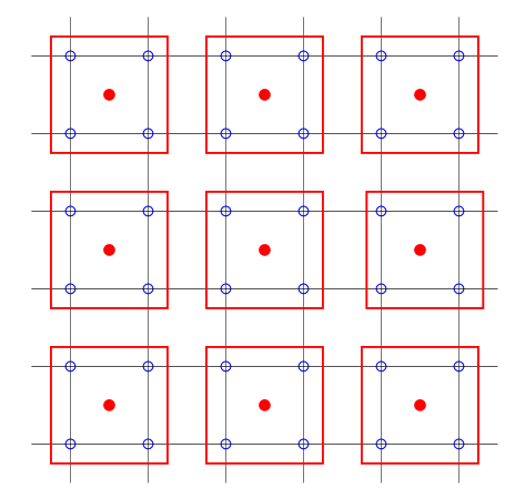
Figure 1: A renormalization group blocking for the square lattice. The original lattice sites are the open circles, the sites after the renormalization transformation are the solid circles.

One widely studied family of kernels is the family of majority rule transformations. If there are an odd number of spins in every block, then $T(\bar{\sigma},\sigma)=1$ if the majority of the spins in each block agree with the block spin and $T(\bar{\sigma},\sigma)=0$ otherwise. If there are an even number of spins in every block, then we let $T(\bar{\sigma},\sigma)$ be the product over the blocks $B$ of

$$t(\bar{\sigma}_{B},\{\sigma_{i}\}_{i\in B})=\cases{1&if \, $\bar{\sigma}_{B}\,\sum_{i\in B}\sigma_{i}>0$\cr 0&if \, $\bar{\sigma}_{B}\,\sum_{i\in B}\sigma_{i}<0$\cr 1/2&if \, $\sum_{i\in B}\sigma_{i}=0$\cr}$$ (3)

where $\bar{\sigma}_{B}$ denotes the block spin for block $B$.

The general approach presented in this paper applies to all these renormalization group maps. The numerical calculations that we will present are for the critical nearest neighbor Ising model on the square lattice with the majority rule renormalization group map with two by two blocks.

3 Renormalized Hamiltonian in the lattice-gas variables

Real-space renormalization group calculations are usually done using the spin variables $\sigma_{i}=\pm 1$. Our method is based on what are sometimes called the lattice-gas variables ${n}_{i}=(1-\sigma_{i})/2$ which take on the values $0,1$. Note that we have made the convention that a spin value of $+1$ corresponds to a lattice gas value of $0$. Throughout this paper we will use $\sigma$’s for spin variables taking on the values $\pm 1$, and ${n}$’s for lattice-gas variables taking on the values $0,1$. We indicate renormalized spins or variables with a bar over them, e.g., $\bar{\sigma}_{i}$, $\bar{n}_{i}$. We use $\sigma$ to denote the entire spin configuration $\{\sigma_{i}\}$. Likewise, ${n}$, $\bar{\sigma}$ and $\bar{n}$ denote the corresponding collections of variables.

In this section we work entirely in the lattice-gas variables, both for the original Hamiltonian and the renormalized Hamiltonian. We write the renormalized Hamiltonian as

$$\bar{H}(\bar{n})=\sum_{Y}\,c(Y)\,\bar{n}(Y)$$ (4)

where the sum is over all finite subsets including the empty set, and

$$\bar{n}(Y)=\prod_{i\in Y}\bar{n}_{i}$$

Consider the block-variable configuration of all $0$’s. Our method for computing the renormalized Hamiltonian uses only block-variable configurations which differ from this configuration at a finite number of sites. For a finite subset $X$, let $\bar{n}^{X}$ denote the block-variable configuration with all block variables in $X$ equal to $1$ and the rest equal to $0$. Then eq. (2) says

$$\exp(-\bar{H}(\bar{n}^{X}))=\sum_{n}\,T(\bar{n}^{X},{n})\,e^{-H({n})}$$

Note that $\bar{n}^{\emptyset}(X)=0$ except when $X=\emptyset$. So $\bar{H}(\bar{n}^{\emptyset})=c(\emptyset)$. In particular, $c(\emptyset)$ will grow as the size of the finite volume. The other coefficients $c(Y)$ should have finite limits in the infinite-volume limit. We define $f(X)$ by

$$f(X)=\bar{H}(\bar{n}^{X})-\bar{H}(\bar{n}^{\emptyset})$$

Then $f(X)$ should have a finite limit in the infinite-volume limit, and it should be related to the infinite-volume $c(X)$ by

$$f(X)=\sum_{Y:\emptyset\neq Y\subset X}c(Y)$$ (5)

The system of equations (5) can be explicitly solved for the $c(Y)$. We claim that the solution for $X\neq\emptyset$ is

$$c(X)=\sum_{Y:\emptyset\neq Y\subset X}(-1)^{|X|-|Y|}\,f(Y)$$ (6)

This is a standard inversion trick. To verify (6), define $c(X)$ by (6). Then for a given $X\neq\emptyset$,

$$\sum_{Y:\emptyset\neq Y\subset X}c(Y) = \sum_{Y:\emptyset\neq Y\subset X}\sum_{Z:\emptyset\neq Z\subset Y}(-1)^{|Y|-|Z|}\,f(Z)$$ (7)

$$= \sum_{Z:\emptyset\neq Z\subset X}\,f(Z)\sum_{Y:Z\subset Y\subset X}(-1)^{|Y|-|Z|}$$

The sum over $Y$ is $1$ if $X=Z$. If $Z$ is a proper subset of $X$, we claim this sum is $0$. To see this:

$$\sum_{Y:Z\subset Y\subset X}(-1)^{|Y|-|Z|}=\sum_{W:W\subset X\setminus Z}(-1)^{|W|}=\prod_{i\in X\setminus Z}(1+(-1))=0$$

Thus (7) collapses to $f(X)$.

The important feature of eq. (6) is that the coefficient $c(X)$ only depends on a finite number of free energies $f(Y)$, specifically those with $Y\subset X$. As we will see, these free energies can be computed extremely accurately. So individual coefficients $c(X)$ in the lattice-gas variables can be computed extremely accurately. Moreover, this computation does not depend on how many terms we decide to keep in the renormalized Hamiltonian. If we increase the number of terms we keep, then the coefficients we have already computed will not change.

We have carried out numerical calculations of a large number of the coefficients in the lattice-gas representation for the critical nearest neighbor Ising model on the square lattice with the majority rule renormalization group map with two by two blocks. We need a criterion for deciding for which $Y$ we will compute $c(Y)$. We assume the coefficients will decay as the number of sites in $Y$ grows and as the distance between these sites grows. So we need a measure of the size of a set $Y$. There is no canonical way to define this size. We use the following ad hoc quantity. If $Y=\{y_{1},y_{2},\cdots,y_{n}\}$, then we define

$$S(Y)=\sum_{i=1}^{n}||y_{i}-c||_{2}^{2}$$ (8)

where $c$ is the center of mass:

$$c={1\over n}\sum_{i=1}^{n}y_{i}$$

and $||\quad||_{2}$ is the usual Euclidean distance in the plane. Note that we do not take a square root in (8).

We claim that if $X^{\prime}\subset X$ then $S(X^{\prime})\leq S(X)$. To prove this it suffices to prove the case that $X^{\prime}$ has one less site than $X$. Let $X$ be $x_{1},x_{2},\cdots,x_{n}$ and $X^{\prime}$ be $x_{1},x_{2},\cdots,x_{n-1}$. Let $c$ be the center of mass of $X$ and $c^{\prime}$ the center of mass of $X^{\prime}$. So

$$S(X^{\prime})=\sum_{i=1}^{n-1}||x_{i}-c^{\prime}||_{2}^{2}$$

The center of mass has the property that it minimizes the above sum. So

$$S(X^{\prime})\leq\sum_{i=1}^{n-1}||x_{i}-c||_{2}^{2}\leq\sum_{i=1}^{n}||x_{i}-c||_{2}^{2}=S(X)$$

We fix a cutoff $C>0$, and compute $c(Y)$ for all $Y$ with $S(Y)\leq C$. We only need to compute it for one $Y$ from each translation class, and so there are a finite number of such $Y$’s. The bulk of the computation is computing the free energies $f(X)$ for $X$ with $S(X)\leq C$. Using eq. (6) to find the $c(Y)$ requires comparatively little computation. The property that $X^{\prime}\subset X\Rightarrow S(X^{\prime})\leq S(X)$, implies that the collection of $X$ for which we must compute $f(X)$ is just the collection of $X$ with $S(X)\leq C$.

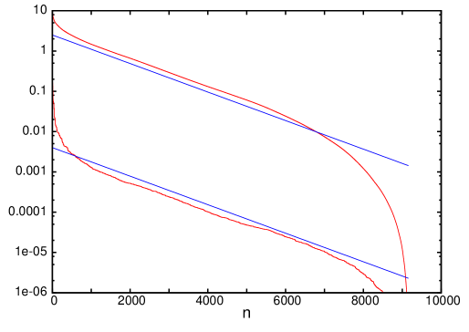
Figure 2: The coefficients $c(Y_{n})$ are ordered so $|c(Y_{n})|$ decreases. The bottom curve is $|c(Y_{n})|$ vs. $n$, and the top curve is the tail $\sum_{i=n}^{N}|c(Y_{n})|$ vs. $n$.

To study how fast the coefficients $c(Y)$ decay, we take one coefficient from each translation class that we have computed and order them so that $|c(Y)|$ is decreasing, i.e., $|c(Y_{n})|\geq|c(Y_{n+1})|$. We then plot $|c(Y_{n})|$ as a function of $n$. This is the bottom curve in figure 2. Note that the vertical axis uses a logarithmic scale. The second quantity plotted (the top curve in the figure) is

$$\sum_{i=n}^{N}|c(Y_{i})|$$

as a function of $n$, where $N$ is the total number of $Y$ for which we compute the coefficients. The two lines shown are given by $c2^{-n/850}$ for two different values of $c$. The two curves in the figure depend on the function $S(Y)$ we use to measure the size of sets and the cutoff we use for this function. However, whatever function and cutoff we use, the resulting curve will be a lower bound on the curve that would result from computing all the coefficients $c(Y)$. In particular, we can make the following observations. The lower curve crosses the horizontal lines at $10^{-2}$, $10^{-3}$ and $10^{-4}$ at $131$,$1223$ and $4023$, respectively. Hence there are at least $131$ translation classes with a coefficient bigger than $10^{-2}$, at least $1223$ with a coefficient bigger than $10^{-3}$, and at least $4023$ with a coefficient bigger than $10^{-4}$.

In the preceding discussion we used one coefficient from each translation class. In addition to the translation symmetry the model is also symmetric under rotations by 90 degrees and relections in lattice axes. More precisely, the additional symmetry is the dihedral group of order 8. We have repeated the previous study of the decay of the coefficients taking into account the dihedral group symmetry as well as the translational symmetry by taking only one term from the above list from each dihedral group symmetry class. The main effect is that the scale on the horizontal axis is reduced by a factor of $8$. This is not surprising since for most subsets, rotations and reflections will generate eight different subsets.

From a mathematical perspective, one would like to show that the renormalized Hamiltonian exists in some Banach space. One choice of norm for the Banach space would be

$$\sum_{Y:0\in Y}|c(Y)|$$

One would like to approximate the Hamiltonian by a Hamiltonian with a finite number of terms. So it is important to see how fast the above sum converges as we include more terms in the Hamiltonian. This is similar to the second plot in figure 2. Note that in this norm each translation class appears $|Y|$ times. So the second plot in figure 2 is in some sense a lower bound on the decay for the Hamiltonian. Another choice of the norm would be

$$\sum_{Y:0\in Y}|c(Y)|e^{\mu(Y)}$$

for some measure $\mu(Y)\geq 0$ of the size of $Y$. For this norm the convergence would be even slower than that seen in the figure.

It is worth noting that norms defined using the lattice-gas representation of the Hamiltonian are in general stronger than norms that use the spin variable representation [5]. For example, if we can write the Hamiltonian in the lattice-gas representation (4) with

$$\sum_{Y\ni 0}\,|c(Y)|<\infty$$

then it is straightforward to show that the Hamiltonian can be represented in the spin variable representation (9) with

$$\sum_{Y\ni 0}\,|d(Y)|<\infty$$

4 Renormalized Hamiltonian in the spin variables

In the previous section we saw that in the lattice-gas variables there is a natural way to compute the coefficients $c(Y)$ in the expansion (4) for $\bar{H}$. In this section we consider the renormalized Hamiltonian in the spin variables:

$$\bar{H}(\bar{\sigma})=\sum_{Y}\,d(Y)\bar{\sigma}(Y)$$ (9)

with $\bar{\sigma}(Y)=\prod_{i\in Y}\bar{\sigma}_{i}$. The sum over $Y$ is over all finite subsets.

We can use $\bar{n}_{i}=(1-\bar{\sigma}_{i})/2$ to express the spin coefficients $d(Y)$ in (9) in terms of the lattice-gas coefficients $c(Y)$ in (4).

$$\bar{H}(\bar{\sigma}) = \sum_{X}c(X)\bar{n}(X)=\sum_{X}c(X)\,2^{-|X|}\prod_{i\in X}(1-\bar{\sigma}_{i})$$

$$= \sum_{X}c(X)\,2^{-|X|}\sum_{Y:Y\subset X}(-1)^{|Y|}\bar{\sigma}(Y)$$

$$= \sum_{Y}\bar{\sigma}(Y)(-1)^{|Y|}\sum_{X:Y\subset X}c(X)\,2^{-|X|}$$

$$= \sum_{Y}d(Y)\,\bar{\sigma}(Y)$$

where the spin coefficients $d(Y)$ are given by

$$d(Y)=(-1)^{|Y|}\sum_{X:Y\subset X}c(X)\,2^{-|X|}$$ (10)

The problem is that to compute the spin coefficient $d(Y)$ we need the lattice-gas coefficients $c(X)$ for infinitely many $X$, and so we need the free energies $f(X)$ for infinitely many $X$’s. So we must introduce some sort of approximation.

Let ${\mathbb{Y}}_{\infty}$ be a collection of finite subsets of the renormalized lattice such that one set from each translation class is contained in ${\mathbb{Y}}_{\infty}$. We can rewrite (9) as

$$\bar{H}(\bar{\sigma})=\sum_{Y\in{\mathbb{Y}}_{\infty}}\,d(Y)\sum_{t}\bar{\sigma}(Y+t)$$

where the sum over $t$ is over the translations for the renormalized lattice. Here $Y+t$ denotes $\{i+t:i\in Y\}$.

Now let ${\mathbb{Y}}$ be a finite subcollection of ${\mathbb{Y}}_{\infty}$. We want to compute an approximation to the above of the form

$$\bar{H}(\bar{\sigma})\approx\sum_{Y\in{\mathbb{Y}}}\,d(Y)\sum_{t}\bar{\sigma}(Y+t)$$

We will consider two methods which we will refer to as the “partially exact” method and the “uniformly close” method.

For the partially exact method, we begin by noting that we can write $\bar{H}(\bar{n})$ as

$$\bar{H}(\bar{n})=\sum_{Y\in{\mathbb{Y}}_{\infty}}\,c(Y)\sum_{t}\bar{n}(Y+t)$$

The approximation is simply to truncate this sum by restricting $Y$ to those in ${\mathbb{Y}}$:

$$\bar{H}(\bar{n})\approx\sum_{Y\in{\mathbb{Y}}}\,c(Y)\sum_{t}\bar{n}(Y+t)$$

The $c(Y)$ are exact. As we saw in the last section we can compute them from (6) by computing the free energies $f(X)$ for $X\in{\mathbb{Y}}$. We then convert this Hamiltonian to the spin variables with no approximation. The result is that the approximation to $\bar{H}(\bar{\sigma})$ is

$$\sum_{Y\in{\mathbb{Y}}}\,d(Y)\sum_{t}\bar{\sigma}(Y+t)$$ (11)

with

$$d(Y)=(-1)^{|Y|}\sum_{X:Y\subset X,X+t\in{\mathbb{Y}}}c(X)\,2^{-|X|}$$ (12)

where the notation $X+t\in{\mathbb{Y}}$ means some translation of $X$ (possibly $X$ itself) is in ${\mathbb{Y}}$. Thus this method is equivalent to truncating the exact formula (10) by restricting the sum over $X$ to sets in ${\mathbb{Y}}$ and their translates. In the lattice-gas variables our approximation to $\bar{H}$ agrees with the true $\bar{H}$ for all $n^{X}$ such that $X\in{\mathbb{Y}}$. The change from lattice gas to spin variables did not involve any approximation, so our approximation to $\bar{H}$ in the spin variables agrees exactly with the true $\bar{H}$ for all configurations $\bar{\sigma}^{Y}$ for $Y\in{\mathbb{Y}}$. This is the reason for calling this method “partially exact.” It is exact for some of the block-spin configurations.

For the uniformly close method let ${\mathbb{X}}$ be another finite collection of finite subsets which contains at most one set from each translation class. We compute the free energies $f(X)$ for $X\in{\mathbb{X}}$, i.e., we compute $\bar{H}(\bar{\sigma}^{X})$. We define the error of a set of coefficients $\{d(Y):Y\in{\mathbb{Y}}\}$ to be

$$\max_{X\in{\mathbb{X}}}|\bar{H}(\bar{\sigma}^{X})-\sum_{Y\in{\mathbb{Y}}}\,d(Y)\sum_{t}\bar{\sigma}^{X}(Y+t)|$$

where $\bar{\sigma}^{X}$ is the spin configuration which is $-1$ on $X$ and $+1$ on all other sites. We then choose the coefficients $d(Y)$ to minimize the above error. This is a standard linear programming problem which we solve by the simplex algorithm. We call this the uniformly close approximation since we have a uniform bound on the difference between our approximation and the exact $\bar{H}$ for the block-spin configurations $\bar{\sigma}^{X}$ for $X\in{\mathbb{X}}$. (For other $X$ we cannot say anything about how well the approximation does.) If ${\mathbb{X}}={\mathbb{Y}}$, then the partially exact approximation makes the above error zero. We only use the uniformly close approximation for ${\mathbb{X}}$ which are larger than ${\mathbb{Y}}$.

We take the following point of view. We think of ${\mathbb{Y}}$ as being fixed. It determines a finite-dimensional space of Hamiltonians that we use to approximate the renormalized Hamiltonian. We then think of the collection ${\mathbb{X}}$ as being variable. A larger ${\mathbb{X}}$ means we “know” more free energies and so have more information to use in computing the approximation. In our studies we will take the collection ${\mathbb{Y}}$ to be all the subsets $Y$ with $s(Y)\leq C_{\bar{H}}$ for some cutoff $C_{\bar{H}}$, and ${\mathbb{X}}$ to be all the $X$ with $s(X)\leq C_{f}$ for some cutoff $C_{f}\geq C_{\bar{H}}$

When we worked in the lattice-gas variables the computation of the coefficients $c(X)$ was unambiguous. The computation of the values of $\bar{H}(\bar{n})$ requires some approximations, but as we will see in section 5 these approximation are well behaved and introduce small errors. The computation of the $c(X)$ from the $\bar{H}(\bar{n})$ does not require any approximation or truncation. In the spin variable representation we now have multiple ways to compute the coefficients $d(X)$ depending on whether we use the partially exact or uniformly close methods and on the choices of ${\mathbb{X}}$ and ${\mathbb{Y}}$. We restrict our study of the spin variable coefficients to studying how these choices affect the values of individual coefficients. We focus our attention on three particular coefficients: the nearest neighbor, the next nearest neighbor and the plaquette. These refer to the coefficients of $\sigma_{i}\sigma_{j}$ with $|i-j|=1$, of $\sigma_{i}\sigma_{j}$ with $|i-j|=\sqrt{2}$, and of $\sigma_{i}\sigma_{j}\sigma_{k}\sigma_{l}$ where $i,j,k,l$ are the corners of a unit square. As in the previous section, our numerical calculations are for the critical nearest neighbor Ising model on the square lattice with the majority rule renormalization group map with two by two blocks.

For the partially exact method we have one parameter - the cutoffs $C_{\bar{H}}$ and $C_{f}$ are equal and correspond to the cutoff $C$ of section 3. So we can plot individual coefficients as a function of $C_{f}$. For the uniformly close method we have two parameters: the cutoff $C_{\bar{H}}$ determines the finite-dimensional subspace used to approximate the renormalized Hamiltonian and the cutoff $C_{f}$ determines the number of $\bar{H}(\bar{n})$ values we use. We plot the coefficients in this case as a function of $C_{f}$ for several different choices of $C_{\bar{H}}$. The results are shown in figures 3,4, and 5. The variations seen in the three coefficients are roughly comparable in size. Note that while the ranges of the vertical axes vary in the three figure, the scales for the vertical axes are all the same. The variations in the coefficients are on the order of several thousandths. So even for these relatively large coefficients, it is difficult to determine the value of the coefficient to better than a few percent. For smaller coefficients the variations are somewhat smaller, but as a fraction of the coefficient they are typically larger.

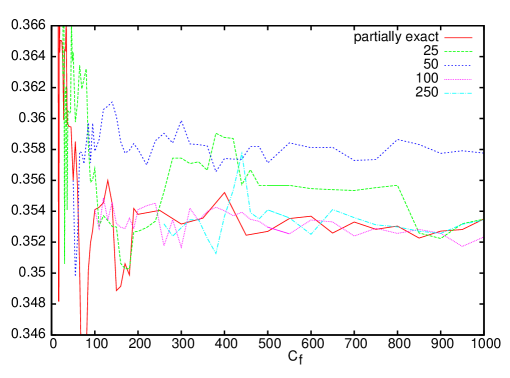
Figure 3: The dependence of the nearest neighbor coefficient in the spin variable representation of the renormalized Hamiltonian on the computation method. The solid curve is the partially exact method. The dashed curves are the uniformly close method with four different choices of $C_{\bar{H}}$

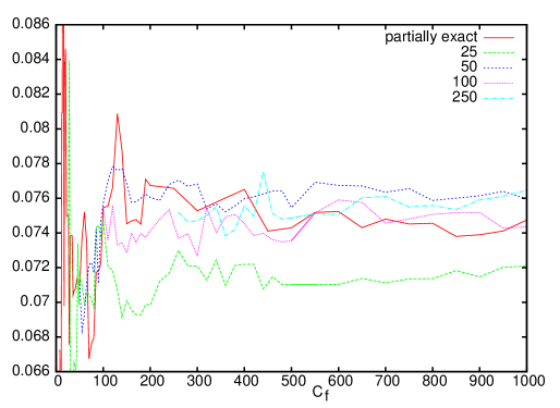
Figure 4: The next nearest neighbor coefficient in the spin variable representation of the renormalized Hamiltonian

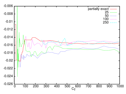
Figure 5: The plaquette coefficient in the spin variable

These three coefficients (along with many others) have of course been computed before. Two early references are [4, 16]. The point of our study is not the values of these coefficients but rather the variation in their values as one varies the method used to compute them.

5 Computing the free energy

Fix a block-spin configuration $\bar{\sigma}$. We want to compute the free energy $\bar{H}(\bar{\sigma})$ of the constrained partition function

$$\exp(-\bar{H}(\bar{\sigma}))=\sum_{\sigma}\,T(\bar{\sigma},\sigma)\,e^{-H(\sigma)}$$

Initially we work with the spin variables, but later in this section we will switch to the lattice-gas variables. We only need to do this computation for configurations $\bar{\sigma}$ which are $+1$ except on a finite set. Even when the original system is at the critical point, these constrained systems have relatively short correlation lengths. This is where the real power of the renormalization group becomes apparent. In particular, finite-volume effects in the above computation decay very quickly as the volume increases.

Before we explain our method for the computation, we first indicate how $\bar{H}(\bar{\sigma})$ can be computed by a Monte Carlo calculation. (We have done such a simulation as a check on the method we describe later.) Fix a relatively small set of block spins, $X$. Let $V$ be a finite volume of block spins containing $X$ which is large enough that the boundary of $V$ is far from $X$. We include only the factors in the renormalization group kernel corresponding to the blocks in $V\setminus B$. For these blocks we take the block spins to be $+1$. We then run a Monte Carlo simulation of the Ising system with this kernel outside of $X$. When we sample the simulation we compute the block-spin configuration on $X$. This allows us to compute the relative weights of the possible block-spin configurations on $X$. From these weights we can then compute the $\bar{H}(\bar{\sigma})$ for $\bar{\sigma}$ which are $-1$ only on a subset of $X$.

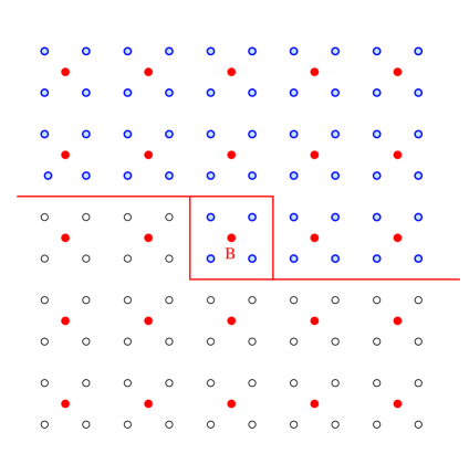
Figure 6: We compute $\bar{H}(\bar{\sigma})$ by summing out the original spins one block at a time. The open circles are spins that have been summed over, while the blue (gray) circles are spins that have yet to be summed over. The red (black) circles are the fixed block spins.

We now turn to our method for computing $\bar{H}(\bar{\sigma})$. It does not involve Monte Carlo methods, and it is much more accurate than the Monte Carlo approach described in the previous paragraph. Everything in the following depends on $\bar{\sigma}$, but we will not make this dependence explicit. Imagine that we have summed over the spins one block at a time in such a way that we have reached the state in figure 6. Open circles indicate sites in the original lattice for which we have already summed over the spin, and blue (gray) circles represent sites for which we have not. (Red (solid) circles indicate the block spins which are fixed throughout this computation.) The result of this partial computation of the free energy is a function of the spins in the original lattice with shaded circles. In fact, it only depends on those that are nearest neighbors of a spin with an open circle. We will refer to these spins as boundary spins. The quantity we have computed so far is positive, and we write it in the form

$$\exp(\sum_{X}a(X)\sigma(X)+\Delta H)\,\prod_{B^{\prime}}t_{B^{\prime}}(\bar{\sigma},\sigma)$$

where $X$ is summed over finite subsets of the boundary spins. $\Delta H$ denotes the terms in the Hamiltonian that only involve spins with shaded circles. (These terms have not yet entered the computation.) The product over $B^{\prime}$ is over the blocks containing shaded circles, and $t_{B^{\prime}}(\bar{\sigma},\sigma)$ is the factor in the renormalization group kernel for block $B^{\prime}$. The next step is to sum over the four spins in the block $B$ and take the logarithm of the result:

$$\ln\left[\sum_{\sigma_{B}}\exp(\sum_{X}a(X)\sigma(X)+\Delta H)\,\prod_{B^{\prime}}t_{B^{\prime}}(\bar{\sigma},\sigma)\right]$$

The sum over $\sigma_{B}$ denotes a sum over the spins $\sigma_{i}$ with $i\in B$. Terms $a(X)\sigma(X)$ for which $X\cap B=\emptyset$ pass through this computation trivially. So do the terms in $\Delta H$ which do not involve a spin in the block $B$ and the factors $t_{B^{\prime}}$ for $B^{\prime}\neq B$. So the computation that we must actually do is

$$\ln\left[\sum_{\sigma_{B}}\exp(\sum_{X:X\cap B\neq\emptyset}a(X)\sigma(X)+h)\,t_{B}(\bar{\sigma},\sigma)\right]$$

where $h$ contains the terms in $H$ that only depend on spins with shaded circles and depend on at least one spin in $B$.

To do this computation numerically, we must introduce a truncation. We fix a finite subset $D$ of the boundary sites centered near $B$. We then restrict the sum over $X$ to $X\subset D$. We need to write the result of the truncated computation in the form

$$\ln\left[\sum_{\sigma_{B}}\exp(\sum_{X:X\cap B\neq\emptyset,X\subset D}a(X)\sigma(X)+h)\,t_{B}(\bar{\sigma},\sigma)\right]=\sum_{Y}a^{\prime}(Y)\sigma(Y)$$

The left side only depends on spins in $D^{\prime}=D\setminus B$, so the sum on the right may be restricted to $Y\subset D^{\prime}$. If we define $F(\sigma)$ to be the left side of this equation, then the coefficients are given by

$$a^{\prime}(Y)=2^{-|D^{\prime}|}\sum_{\sigma_{D^{\prime}}}F(\sigma)$$

The amount of computation required grows quite rapidly as $D$ grows for three reasons. First, the number of $X$ with $X\subset D$ grows as $2^{|D|}$. Second, the sum over $\sigma_{D^{\prime}}$ in the above also grows as $2^{|D|}$. Third, the number of $Y$ also grows as $2^{|D|}$. We have found that $a(X)$ decays quickly as the number of sites in $X$ grows. So we can make a further truncation by only keeping terms $a(X)$ with $|X|$ less than some specified cutoff. ($|X|$ denotes the number of sites in $X$.) This greatly reduces the growth of the computation with $D$ from the first and third effects. But we are still left with the second effect.

We can eliminate the second effect by working in the lattice-gas variables. We replace $\sum_{X}a(X)\sigma(X)$ by $\sum_{X}b(X){n}(X)$. Define

$$F({n})=\ln\left[\sum_{{n}_{B}}\exp(\sum_{X:X\cap B\neq\emptyset,X\subset D}b(X){n}(X)+h)\,t_{B}(\bar{n},{n})\right]$$ (13)

We need to compute the coefficients in

$$F({n})=\sum_{X}b^{\prime}(X){n}(X)$$

As we saw in section 3, they are given by

$$b^{\prime}(X)=\sum_{Y:\emptyset\neq Y\subset X}(-1)^{|X|-|Y|}\,F(n^{Y})$$ (14)

where $n^{Y}$ is the configuration that is $1$ on $Y$ and $0$ off of it. So to compute $b^{\prime}(X)$ we only need to compute $F(n^{Y})$ for $Y\subset X$.

In this approach using the lattice-gas variables we can forget about the set $D$ entirely. Instead we specify a finite collection ${\mathbb{B}}$ of subsets of the boundary spins with the property that they intersect $B$. We then make the approximation

$$\sum_{X:X\cap B\neq\emptyset}b(X){n}(X)\approx\sum_{X\in{\mathbb{B}}:X\cap B\neq\emptyset}b(X){n}(X)$$ (15)

We use (14) to compute $b^{\prime}(X)$. It will be nonzero only for $X\subset D^{\prime}$. Before we sum over the next block of spins, we need to truncate $\sum_{X}b^{\prime}(X){n}(X)$. We keep only the terms such that $X$ is in ${\mathbb{B}}+t$ where $t$ is the translation that takes the block we just summed over to the block we are summing over next, and ${\mathbb{B}}+t$ denotes the collection of sets of the form $X+t$ for $X\in{\mathbb{B}}$.

We take the finite collection ${\mathbb{B}}$ to be all $X$ which intersect $B$ and satisfy $S(X)\leq C_{B}$ where $S(X)$ is some size function and $C_{B}$ is some cutoff. We use the size function given by (8) that we used for choosing the block-spin sets. In our calculations we take $C_{B}=260$ which leads to $10,763$ sets in the collection ${\mathbb{B}}$. We discuss the effect of $C_{B}$ on the error in the following section.

The above discussion took place in an infinite volume. The region shown in figure 6 is a finite piece of the infinite volume. In practice we can only sum over the spins in a finite number of blocks. The block-spin configuration $\bar{n}$ is of the form $\bar{n}^{Y}$ for a finite set $Y$. We carry out the computation in a finite volume which is chosen so that the distance from $Y$ to the boundary of the finite volume is sufficiently large. We will study how large the finite volume should be in the next section.

6 Errors

In this section we study the sources of error in our computations of the $f(X)$. There are two: the use of a finite volume to compute infinite-volume quantities and the truncation determined by the cutoff $C_{B}$ in section 5.

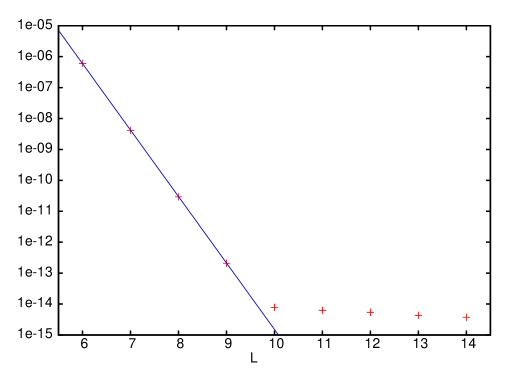
Figure 7: $L$ is a measure of the size of the finite volume. The quantity plotted is the average change in $f(X)$ when $L$ is decreased by $1$. (See eq. (16).)

We choose the finite volume in which we carry out our calculation as follows. The block-spin configurations $\bar{n}$ that we consider are of the form $\bar{n}^{Y}$ for finite sets $Y$. We take these sets $Y$ to be centered near the origin and take the finite volume to be a square centered at the origin. The square contains the blocks with centers at $(2i,2j)$ with $-L\leq i\leq L$, $-L\leq j\leq L$. So the infinite-volume limit is obtained by taking $L\rightarrow\infty$.

To study the finite-volume error in our calculation we do the following. The free energy $f(Y)$ depends on $L$, so we denote it by $f_{L}(Y)$. As a measure of the finite-volume error we use

$${1\over N}\sum_{Y}|f_{L}(Y)-f_{L-1}(Y)|$$ (16)

where the sum is over one element of each translation class with $s(Y)\leq 210$, and $N$ is the number of terms in the sum. In this study of the finite-volume error we take $C_{B}=30$. This is much smaller than the cutoff we used for the main calculations, but the behavior of the finite-volume error with $L$ is the same whether we look at this smaller set of coefficients or the larger set.

This average difference as a function of $L$ is shown in figure 7. The vertical scale is logarithmic, so the approximately linear dependence seen for the smaller values of $L$ indicates exponential decay of this difference with $L$. The line shown in the figure is of the form $ce^{-L/0.2}$. Keeping in mind that $L$ corresponds to numbers of blocks and the blocks are $2$ by $2$, the decay length of $0.2$ corresponds to a decay length of $0.4$ in units of lattice spacings. This very short decay length is a result of the block spin being $+1$ at all but a finite number of block sites. Beginning with $L$ around 10 the difference is dominated by numerical errors. In our simulations we are very conservative and take $L=15$. With this choice the finite-volume error is at the same level as the numerical error.

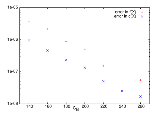
Figure 8: We plot the average of $f(X)-\bar{f}(X)$, as defined by eq. (17), and of $c(X)-\bar{c}(X)$, as defined by eq. (18), as a function of the cutoff $C_{B}$.

The translational symmetry of the original model implies that $f(X)$ is unchanged if we translate $X$. So we only need to compute $f(X)$ for one element of each translation class. The model is also invariant under the dihedral group symmetry generated by rotations by mutiples of $\pi/2$ and reflections in the coordinate axes. However, our method of computing $f(X)$ breaks the dihedral symmetry of the lattice, so our values of $f(X)$ for $X$’s from the same dihedral class are not exactly the same. The dihedral symmetry is only restored when we let $L\rightarrow\infty$ and $C_{B}\rightarrow\infty$. We have already seen that we can take $L$ sufficiently large that the finite-volume error is reduced to the order of the numerical error. So we can use the breaking of the dihedral symmetry to study how the error depends on the cutoff $C_{B}$.

For various choices of $C_{B}$ we compute $f(X)$ for the same collection of $X$ as in our main calculation. Let $\bar{f}(X)$ be the average of $f(Y)$ over one $Y$ from each translation class which is related to $X$ by the dihedral symmetry. (The number of terms involved in this average ranges from $1$ to $8$.) The differences $f(X)-\bar{f}(X)$ are a measure of the amount of breaking of the dihedral symmetry and hence of the error in the computation from the cutoff $C_{B}$. We use the average

$${1\over N}\sum_{Y}|f(Y)-\bar{f}(Y)|$$ (17)

to quantify the error. As before the sum is over one element of each translation class with $s(Y)\leq 210$, and $N$ is the number of terms in the sum. This quantity is plotted in figure 8 as a function of $C_{B}$ for the free energies $f(Y)$. It is the higher set of points. For the coefficients in the lattice-gas variables we define $\bar{c}(X)$ analogously, and study the average

$${1\over N}\sum_{Y}|c(Y)-\bar{c}(Y)|$$ (18)

This quantity is the lower set of points in figure 8.

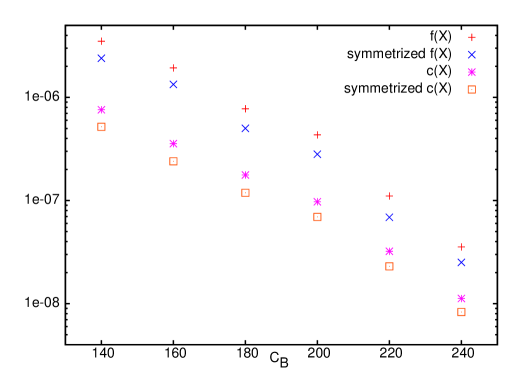
Figure 9: The convergence of four different quantities as $C_{B}\rightarrow\infty$. From top to bottom the four quantities are given by equations (19) to (22).

We also study the convergence as $C_{B}\rightarrow\infty$ in another way. Let $f^{\infty}(Y)$ denote $f(Y)$ for the largest value of $C_{B}$ which we use, i.e., 260. We then consider

$${1\over N}\sum_{Y}|f(Y)-f^{\infty}(Y)|$$ (19)

This is plotted as a function of $C_{B}$ in figure 9 for the free energy $f(Y)$. We also plot

$${1\over N}\sum_{Y}|\bar{f}(Y)-\bar{f}^{\infty}(Y)|$$ (20)

As the figure shows, averaging over the dihedral group like this reduces the error somewhat. The figure also includes the analogous plots for the coefficients in the lattice-gas representation, i.e., of the quantities

$${1\over N}\sum_{Y}|c(Y)-c^{\infty}(Y)|$$ (21)

and

$${1\over N}\sum_{Y}|\bar{c}(Y)-\bar{c}^{\infty}(Y)|$$ (22)

7 Conclusions:

We have shown that if we use lattice-gas variables, then the computation of the coefficients in the renormalized Hamiltonian only depends on a finite number of values of the renormalized Hamiltonian. So this computation does not depend on how we approximate the inherently infinite-dimensional renormalized Hamiltonian by a finite-dimensional approximation. We have also given a highly accurate method for computing the values of the renormalized Hamiltonian which takes advantage of the finite correlation length that results from the introduction of the renormalization group transformation.

The renormalized Hamiltonian has infinitely many different terms but the conventional wisdom is that it may be well approximated by a finite number of terms. In particular, the magnitude of the coefficients should decay as the “size” of the set of lattice sites increases. We studied this for the nearest neighbor critical Ising model on the square lattice under one step of the majority rule renormalization group transformation. We computed a large number of coefficients in the lattice-gas variables, ordered them by decreasing magnitude and plotted them. We found that over several orders of magnitude the coefficients decayed exponentially with the number of terms, but the decay rate was slow. It takes about $850$ additional terms to see the magnitude reduced by just a factor of $1/2$.

If we use the usual spin variables, there is no natural way to compute the coefficients of the renormalized Hamiltonian. We considered two methods of truncation. If we look at an individual coefficient, we see significant dependence on the method used and on the value of the cutoffs used to specify the truncations in these methods. Even with our computation of approximately $10,000$ values of the renormalized Hamiltonian, the uncertainty in the spin variable coefficients due to the different truncation methods is on the order of a percent for the largest coefficients and even larger as a percentage for some of the smaller coefficients.

One might hope to prove theorems about these real-space renormalization group transformations by defining a suitable Banach space of Hamiltonians and then doing a computer aided proof to show the transformation is defined in some open subset of the Banach space and there is a fixed point in this subset. Proving there is a fixed point would require constructing an approximation to the fixed point with a finite number of terms. Our numerical results suggest that at best such an approach will require a huge number of terms in the finite approximation and at worst the number of terms needed will doom the approach to failure.

Past numerical studies of the two dimensional Ising model using the renormalization group have produced fairly accurate values of the critical exponents using a relatively modest number of terms in the renormalized Hamiltonian. These studies use the spin variables, so their accuracy is surprising given the difficulty we have found in computing the coefficients in the renormalized Hamiltonian accurately. An interesting question is to understand this.

References

- [1]
- [2] A. Brandt and D. Ron, Renormalization multigrid (RMG): statistically optimal renormalization group flow and coarse-to-fine Monte Carlo acceleration, J. Stat. Phys. 102, 231-257 (2001).
- [3] R. B. Griffiths and P. A. Pearce, Mathematical properties of position-space renormalization-group transformations, J. Stat. Phys. 20, 499-545 (1979).
- [4] R. Gupta and R.Cordery, Monte Carlo renormalized Hamiltonian Phys. Lett. 105A, 415-417 (1984).
- [5] R. B. Israel, Convexity in the theory of lattice gases (Princeton University Press, Princeton, 1979).
- [6] R. B. Israel, Banach algebras and Kadanoff transformations, in: Random Fields (Esztergom, 1979), vol. II, J. Fritz, J. L. Lebowitz, D. Szász, (eds.), (North-Holland,1981).
- [7] I. A. Kashapov, Justification of the renormalization - group method, Theor. Math. Phys. 42, 184-186 (1980).
- [8] T. Kennedy, Some rigorous results on majority rule renormalization group transformations near the critical point, J. Stat. Phys. 72, 15-37 (1993).
- [9] T. Kennedy and K. Haller, Absence of renormalization group pathologies near the critical temperature - two examples, J. Stat. Phys. 85, 607-637 (1996).
- [10] D. Ron and R. H. Swendsen, Calculation of effective Hamiltonians for renormalized or non-Hamiltonian systems, Phys. Rev E 63, 066128 (2001).
- [11] D. Ron and R. H. Swendsen, Importance of multispin couplings in renormalized Hamiltonians Phys. Rev E 66, 056106 (2002).
- [12] D. Ron,R. H. Swendsen and A. Brandt, Inverse Monte Carlo renormalization group transformations for critical phenomena, Phys. Rev. Lett. 89, 275701 (2002).
- [13] D. Ron,R. H. Swendsen and A. Brandt, Computer simulations at the fixed point using an inverse renormalization group transformation, Physica A 346, 387-399 (2005).
- [14] R. Shankar, R. Gupta, and G. Murthy, Dealing with truncation in Monte Carlo renormalization-group calculations, Phys. Rev. Lett. 55, 1812-1815 (1985).
- [15] R. Swendsen, Monte Carlo renormalization group, Phys. Rev. Lett. 42, 859-861 (1979).
- [16] R. Swendsen, Monte Carlo calculation of renormalized coupling parameters. I. Ising model, Phys. Rev. B 30, 3866-3874 (1984).
- [17] A. C. D. van Enter, R. Fernández and A. D. Sokal, Regularity properties and pathologies of position-space renormalization - group transformations: scope and limitations of Gibbsian theory, J. Stat. Phys. 72, 879-1167 (1993).
- [18] A. C. D. van Enter, Ill-Defined Block-Spin Transformations at Arbitrarily High Temperatures, J. Stat. Phys. 83, 761-765 (1996).