Difference imaging photometry of blended gravitational microlensing events with a numerical kernel

Abstract

The numerical kernel approach to difference imaging has been implemented and applied to gravitational microlensing events observed by the PLANET collaboration. The effect of an error in the source-star coordinates is explored and a new algorithm is presented for determining the precise coordinates of the microlens in blended events, essential for accurate photometry of difference images. It is shown how the photometric reference flux need not be measured directly from the reference image but can be obtained from measurements of the difference images combined with knowledge of the statistical flux uncertainties. The improved performance of the new algorithm, relative to ISIS2, is demonstrated.

1 Introduction

Over the last 15 years, gravitational microlensing (Einstein, 1936) has been observed routinely and used in the study of dark baryonic matter (Alcock et al., 1993; Aubourg et al., 1993) and stellar atmospheres (Albrow et al., 1999, 2001a, 2001b; Fields et al., 2003; Cassan et al., 2004), and in the search for extrasolar planets (Albrow et al., 2000, 2001c; Gaudi et al., 2002; Bond et al., 2004; Udalski et al., 2005; Beaulieu et al., 2006; Dong et al., 2008; Gaudi et al., 2008). The PLANET collaboration (Albrow et al., 1998) operates a number of 1-m class telescopes distributed around the Southern Hemisphere and performs round-the-clock CCD photometry of microlensing events that have been discovered and alerted in real time by the OGLE (Udalski et al., 1994; Udalski, 2003) and MOA (Bond et al., 2002) microlensing surveys.

In this paper we discuss recent advances in the PLANET difference imaging reduction pipeline, focussing on several subtleties inherent in the reduction of blended microlensing events. In what follows we use the convention

$$D=\frac{R\otimes K-T}{\sum_{ij}K_{ij}}\,$$ (1)

for difference image $D$, reference image $R$, target image $T$ and convolution kernel $K$. That is, a difference image is defined as the convolved reference minus the target, normalised so that it is on the effective exposure scale of the reference.

We illustrate the methods using a sample dataset of images of microlensing event OGLE 2008-BLG-229 that were taken using the Elizabeth 1.0-m telescope at the South African Astronomical Observatory during PLANET operations in 2008. The microlensing event was alerted by OGLE on 2008 May 3 and initially was predicted to have low magnification. Subsequent observations revealed a blended moderate magnification event, peaking with magnification $A_{0}=7.24$ on 2008 July 18. OGLE data and parameters for the event can be obtained from the OGLE Early Warning System website . The SAAO observations consist of 84 images, spanning the time from 7 days before maximum until 23 days after maximum.

2 The reduction pipeline

2.1 Introduction

In our first years of operation, PLANET photometry was performed both in real-time at the telescopes and offline using the DoPHOT PSF-fitting code (Schechter et al., 1993) under a reduction pipeline written mainly by JPB. Following the development of the ISIS code (Alard & Lupton, 1998), we adopted the difference imaging method for obtaining our best photometry offline, while still employing the DoPHOT pipeline at the telescope sites. In the 2006 season, we began using a difference imaging photometric pipeline at the telescope sites and for our final offline photometry. The offline version, known as pySIS2, was developed by MDA, and is based on the ISIS 2 code of Alard (2000). An adaptation of pySIS by CC, known as WISIS, is used for most of the real-time at-telescope reductions, while the pySIS2 code is used at the Perth Observatory. The pipelines allow single images to be reduced immediately after observation using an existing reference template. As better quality images are acquired, the reference template can be updated and the previously observed images rereduced.

2.2 Image registration

The ISIS code requires that all images be fully registered to an astrometric reference. Bright stars are located on all frames and cross-correlation of their positions followed by an iterative rejection scheme is used to define an astrometric transformation for each target image.

An innovation introduced to our offline pipeline in 2007 was the removal of the requirement to fully register images. Instead, we register the images only by a shift in X and Y to the nearest pixel, thus avoiding the need for interpolation and resampling. Resampling is generally undesirable since it introduces correlations between adjacent pixels, meaning that their flux uncertainties are no longer described by Poisson statistics. In the case of images that are close to or below critical spatial sampling, resampling introduces an artifact where stellar PSF’s are not constant or slowly-varying across an image, but depend on the subpixel location of their centroids. Such images usually do not subtract cleanly. Integer-pixel registration was handled in our modified version of ISIS by offsetting the kernel centroid by the subpixel registration residual. We note that this approach is somewhat less flexible than the standard ISIS code, in that it cannot work with sets of images with rotations relative to each other.

2.3 Difference imaging with a numerical kernel

In 2008, we have developed a new version of the code, pySIS3, that is no longer based on ISIS image subtraction. Instead, for the difference-imaging step, we have implemented the algorithm of Bramich (2008). In this method, the kernel is represented as a numerical pixel array, rather than the decomposition of Gaussians multiplied by polynomials used in ISIS. The numerical kernel is able to accommodate images with irregular PSFs, for instance trailed images, that ISIS cannot cope with. An implicit feature of the method is that complete registration is not required and the kernel naturally incorporates subpixel offsets. Image registration in pySIS3 is hence restricted to integer pixel shifts. Bramich (2008) shows examples of how the new algorithm outperforms ISIS. DMB’s code has been used successfully to discover new variable stars in the globular cluster NGC 6366 (Arellano Ferro et al., 2008).

Our implementation has been used for the analysis of several microlensing events, appearing in forthcoming papers on MOA 2007-BLG-197 (Cassan et al., 2009), OGLE 2004-BLG-482 (Zub et al., 2009), and OGLE 2007-BLG-472 (Kains et al., 2008), and for a transit search (Miller et al., 2009). There are several specific details of our implementation that we note here.

First, the algorithm is generally more computationally intensive than ISIS, and the computation time scales strongly with the number of pixels required for the kernel array. For microlensing events, we generally reduce only a subsection of the images, typically 250 x 250 pixels centred on the microlens. Our plate scales are typically around 0.3 arcsec/pixel.

Second, results depend on the size of the pixel array chosen for the kernel. The kernel needs to be large enough to encapsulate the transformation between reference and target, but not so large that it introduces noise into the convolution. We have found the best results by employing a circular kernel with a radius (in pixels) given by

$$R_{\rm kernel}=\min\left(7,4\left({\rm FWHM_{target}-FWHM_{reference}}\right)\right)\,$$ (2)

where ${\rm FWHM_{target}}$ and ${\rm FWHM_{reference}}$ are the full-width at half-maxima (in pixel units) of the microlens on the target and reference images. Regions of the kernel that are located more that 7 pixels from its centre are represented by 3x3 binned pixels in order to reduce noise. The values for the binned kernel pixels are computed from the equations in Bramich (2008) but using a $3\times 3$ boxcar-smoothed version of the reference image.

Third, to prevent saturated stars that have irregular PSFs from entering the kernel determination, we mask a circular area of radius 15 pixels around all pixels that are saturated in either the reference or target image as well as masking the microlens itself. The default behavior is to use all the remaining image pixels to determine the kernel using the Bramich (2008) algorithm. In cases where images are contaminated by artifacts, such as diffraction spikes, that are not easily masked, we have found that using ‘stamps’ around bright unsaturated stars rather than the entire unmasked image renders a kernel that is less prone to contamination.

Fourth, the photometric scaling factor,

$$s\equiv\sum_{ij}K_{ij}\,$$ (3)

where $K$ is the convolution kernel, represents the relative difference in effective exposure time between the reference and target images, i.e. it accounts for differences in both exposure time and atmospheric transparency. For each target, if $s$ is significantly different from the ratio of true exposure times, this usually indicates a poorly subtracted target or one affected by cloud.

Fifth, for images that have poor spatial sampling - either close to or even below critical sampling - we use the following technique. The registered images are oversampled by a factor of two in each direction using cubic O-MOMS interpolation (Blu et al., 2001). This type of resampling does not transfer flux across original-pixel boundaries. A stack of typically 10 of the best of these images are then mapped onto the best-seeing image and combined to make a reference image. Since our individual images usually have random subpixel dithers, this process generally results in an oversampled reference so long as the initial undersampling is not too severe. This approach is similar to that employed in R. Gilliland’s code for difference-imaging of undersampled HST WFPC2 images (Gilliland et al., 2000; Albrow et al., 2001d). We note that this approach is still under development and is not used for the sample data set of images for OGLE 2008-BLG-229 in this paper, which are not undersampled.

2.4 Photometry

To extract photometric measurements from our difference images, we first use the Bphot program from ISIS to compute the PSF of the reference image. This PSF is then convolved with the previously-computed kernel to produce a PSF for each target image. The PSF is then normalised and resampled at the subpixel lens coordinates using cubic O-MOMS interpolation. Any residual background is removed from the difference image using a low-order polynomial model. Finally, the PSF is fitted to the difference image using optimal extraction, i.e each pixel weighted by the inverse of its flux variance.

2.4.1 Flux errors from imprecise coordinates

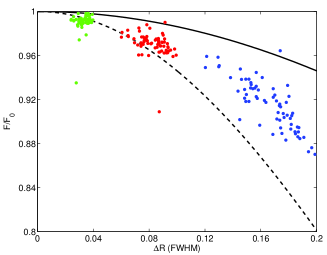
Figure 1: Flux determined at offset coordinates relative to the flux at the correct coordinates as a function of coordinate offset, $\Delta R$ in units of PSF full-width at half-maximum (FWHM). Solid line for unweighted PSF-fitting, dashed line for optimal PSF-fitting with zero background, both under the assumption of a Gaussian PSF. The three distinct groups of data points are computed from the SAAO difference images for OGLE 2008-BLG-229, with the PSF shifted in $x$ by 0.2 (green), 0.5 (red) and 1.0 pixels (blue) (0.06, 0.16, 0.31 arcsec respectively) from their correct value.

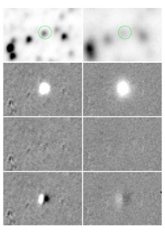
Figure 2: Sample images 78 (left; good seeing) and 83 (right; poor seeing) from the SAAO observations of OGLE 2008-BLG-229. Top row: direct images registered to the nearest pixel, linear greyscale encompassing 95% of pixel values. Second row: difference images, linear greyscale range -400 to +400. Third row: difference images after subtraction of PSF fitted at correct coordinates. Bottom row: difference images after subtraction of PSF fitted at coordinates shifted by +1 pixel in X.

All of the microlensing events towards the Galactic Bulge are blended to some extent in regular ground-based imaging, i.e. the PSF of the microlensed source star overlaps with nearby stars. One implication of this is that the coordinates of the true source star are often displaced by perhaps several tenths of an arcsec from the centroid of the PSF.

When performing photometry on a set of difference images by PSF-fitting, small errors in target location lead to systematic underestimates of the flux. In Figure 1 we show how the flux measurement depends on coordinate displacement, $\Delta R$ (measured in units of FWHM), under a Gaussian PSF assumption. The two limiting cases, shown as lines, are (a) optimal PSF fitting in the zero-background limit and (b) unweighted PSF fitting, essentially the background-limited case. In both limits, the flux error scales as the square of the ratio of the coordinate error to the FWHM of the PSF. This means that a flux error due to an incorrectly-positioned PSF is more serious for images with better seeing and that such a coordinate error introduces scatter into a lightcurve derived from a set of variable-seeing (or even variable-background) images.

We can demonstrate this effect using our test case of SAAO OGLE 2008-BLG-229. We have created difference images using as a reference template a single good-seeing image, number 18, acquired close to the peak of the microlensing event. We have performed optimal photometry on the set of difference images at the correct coordinates (i.e. zero-offset) and again with the coordinates shifted in X by 0.2, 0.5 and 1.0 pixels (0.06, 0.16, 0.31 arcsec) from their correct position. The three displayed groups of data points in Figure 1 show the flux measured at the offset coordinates relative to the flux at the correct position for the three sets of displaced-coordinate measurements. The figure shows that, as predicted, the measured difference flux decreases and its dispersion increases with coordinate offset.

It is important to note that, for difference-image photometry, the above effect applies to difference fluxes, $\Delta F_{i}$. The total flux is given by $F_{i}=F_{0}-\Delta F_{i}$, where $F_{0}$ is the flux on the reference image, $R$ in Eqn (1). This means that the place in the lightcurve where coordinate errors are manifested most strongly depends on the choice of reference image. The flux error is largest for regions of the lightcurve where the magnification is most different from that of the reference image. Consequently, such errors can be minimized for a given part of a lightcurve (for instance some part of a lightcurve suspected to display an anomaly) by choosing a reference image where the source star has a similar magnification.

2.4.2 Precise coordinates for blended events

For high-magnification events, the true source location may be discerned from images taken near peak magnification, when the flux from the true microlensed source star dominates that from nearby blended stars. For data sets comprised of images that have precise registration, a sum of the absolute values of the difference images can be used successfully to refine the coordinates from their initial estimate, even for relatively low-magnification events. This method was used in pySIS2.

In our current circumstance, we have sets of images that are registered only to the nearest pixel. The method of stacking difference images could, in principle, be applied to this data, provided each of the difference images is first shifted by the subpixel registration residual. However, such a shift requires accurate knowledge of the subpixel residuals and involves interpolation and resampling, a process that is inaccurate for images with near- or below-critical spatial sampling.

A better way, that retains the original sampling, is to use the residuals from PSF-fits to the difference images. In appendix A we introduce a new algorithm to refine the source-star coordinates by minimising these residuals over all images. In our photometric code, the algorithm operates as an integral part of the measurement process.

In Figure 2 we show direct, difference and residual images for two sample observations, numbered 78 (good seeing) and 83 (poor seeing) in the SAAO data set for OGLE 2008-BLG-229. Both images were taken during the final days of data, when the source was at a magnification, $A\approx 2.5$. The reference image was again image number 18, taken near peak magnification, $A\approx 7$.

Our coordinate algorithm resulted in a change of 0.54 pixels (0.17 arcsec) in the location of the target star relative to the position found from our best-seeing image (which was adopted as the astrometric reference). Using the correct coordinates, the residual images (difference images after subtraction of the fitted PSF) are very clean.

The effect of a coordinate offset of 1 pixel (0.3 arcsec) is to produce a residual image with large positive and negative flux features remaining. The effect of such an offset on the lightcurve can be tested. We compare difference-flux lightcurves in a blend-free way by mapping them to a point-source point-mass lens model as follows. At time $t_{i}$, the unblended flux from the source star is given by

$$F_{i}=A_{i}F_{\rm base}=F_{0}-\Delta F_{i}\,$$ (4)

where $A_{i}$ is the magnification that we constrain to be defined by the OGLE geometric parameters for the event ($u_{0}$ = 0.139, $t_{\rm E}$ = 53.994 d, $t_{0}$ = JD2454665.780), $F_{0}$ is the unblended source flux on the reference image and $F_{\rm base}$ is the unblended baseline source flux. For each lightcurve, we solve for $F_{0}$ and $F_{\rm base}$by minimizing

$$\chi^{2}\equiv\sum_{i}\frac{\left(A_{i}F_{\rm base}-F_{0}+\Delta F_{i}\right)^{2}}{\sigma_{i}^{2}}$$ (5)

Lightcurves for the whole data set are shown in Figure 3 for the correct coordinates and for those with a 1-pixel offset. An increased scatter is visible in the lightcurve corresponding to the offset coordinates. In the same figure, we also show the best lightcurves we have derived using a template created from the 10 best-seeing images using pySIS3 and ISIS2. Figure 4 shows the corresponding residuals. The effect of a coordinate error can be seen through comparison of the upper two panels, particularly during the last 10 days data points when the magnification is most different from that of the reference image. The superior performance of the new numerical-kernel algorithm can be discerned through comparison of the two lower panels, where the ISIS2 lightcurve residuals (panel (d)) have a 53% greater RMS scatter than the pySIS3 residuals (panel (c)). We note that there is an apparent systematic residual in all the displayed lightcurves, where the earliest data points lie below the magnification curve. This is likely due to the fact that we have constrained, rather than fitted, the underlying geometric model.

2.4.3 Reference flux

The output of our difference-image photometry is the difference in flux, $\Delta F_{i}$, between each target image, $i$, and a photometric reference image. The reference image may be a single observation, as in the preceding sections, but more commonly is created from a combination of images with the best seeing and lowest sky background. In order to interpret our observations we require the flux, $F_{i}=F_{0}-\Delta F_{i}$, where $F_{0}$ is the flux on the reference image. In a model-dependent sense, a deblended $F_{0}$ can be derived as a fitting parameter as done above. More usually, particularly during the time when observations are being acquired, $F_{0}$ is measured from a PSF-fit at the lens coordinates on the reference image. Often this estimation is in error due to the crowded nature of the Galactic Bulge fields in which we observe.

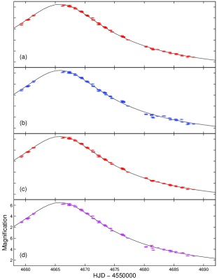
Figure 3: Lightcurves for OGLE 2008-BLG-229: (a) using single template image from near peak, (b) as for (a) but with a 1 pixel coordinate offset, (c) combination of 10 images for reference template, (d) best lightcurve obtained using ISIS2.

An incorrect value for $F_{0}$ can, to some extent, be compensated for in the microlens blend fraction,

$$f_{\rm bl}\equiv\frac{F_{s}}{F_{s}+F_{b}}\,$$ (6)

where for magnification $A$, the baseline flux $(F_{s}+F_{b})$ increases to

$$F=F_{s}A+F_{b}=\left(F_{s}+F_{b}\right)\left(f_{\rm bl}A+\left(1-f_{\rm bl}\right)\right)\$$ (7)

and the blend fraction is derived from lightcurve fitting. However, blending parameters so derived are inconsistent between different datasets for the same event, may take on non-physical values, and certainly no-longer have the correct physical interpretation as the fraction of light contributing to the stellar PSF at baseline from the microlensing source star.

A more-successful approach that we have developed is to choose $F_{0}$ so that the photometric uncertainties in the set of $\Delta F_{i}$ measurements are consistent with Poisson noise for fluxes $F_{i}=F_{0}-\Delta F_{i}$. The algorithm for this determination, referred to as the Poisson reference flux is detailed in Appendix B. The method uses information from all suitable images and the variance in the Poisson reference flux scales roughly with the inverse of the number of images. This variance is generally smaller than the variance for a direct flux measurement from the reference image, which scales with the inverse of the number of individual images incorporated into the reference. For our sample lightcurve, the reference flux is measured directly as $F_{0}=101,820\pm 90$ ADU (likely to include extra blended light), while the poisson method yields $F_{0}=93,570\pm 40$ ADU.

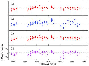
Figure 4: Lightcurve residuals for OGLE 2008-BLG-229 corresponding to Fig 3 after subtraction of a best-fit PSPL model with the geometric parameters set to be those found from OGLE. Errorbars are suppressed for clarity.

3 Summary

Difference imaging has proved to be a powerful technique in the measurement of gravitational microlensing flux variations and for variable stars and transiting extrasolar planets. The numerical kernel method introduced by Bramich (2008) represents a significant advance over the analytic kernel of Alard & Lupton (1998).

In this paper we have shown that, for blended microlensing events, precise determination of the coordinates of the microlens is necessary to obtain accurate photometry. We have presented a new algorithm, based on photometric residuals, to measure such coordinates to high precision.

Additionally, we have introduced a new method to measure the reference flux in a manner that does not depend on an (often inaccurate) analysis of the photometric reference image. The Poisson reference flux method produces a more accurate and precise determination of the unmagnified source flux than a direct measurement from the reference image.

A comparison has been made between photometry from our new code and photometry using ISIS for SAAO images of microlensing event OGLE 2008-BLG-229. The new code produces measurements that display significantly less scatter about a point-source point-mass-lens lightcurve based on the OGLE-determined geometric parameters for the event.

Appendix A Refining the lens position

A.1 target position from a single difference image

We wish to find sub-pixel offsets, $\Delta x$ and $\Delta y$, that create the best match of a PSF model ${P}$ to a difference image ${D}$. Expand the PSF model to first order in $\Delta x$ and $\Delta y$,

$$\mbox{\boldmath${P}$}=\mbox{\boldmath${P}$}_{0}+\Delta x\,\mbox{\boldmath${P}$}_{x}+\Delta y\,\mbox{\boldmath${P}$}_{y}\ ,$$ (8)

and thereby write the residual image as

$$\mbox{\boldmath${R}$}=\mbox{\boldmath${D}$}-\Delta F\,\mbox{\boldmath${P}$}\ ,$$ (9)

where $\mbox{\boldmath${P}$}_{0}$ is the unshifted PSF, $\Delta F$ is the difference flux, and the $x$ and $y$ gradients of the unshifted PSF are

$$\mbox{\boldmath${P}$}_{x}\equiv\mbox{$\frac{\displaystyle{\partial\mbox{\boldmath${P}$}_{0}}}{\displaystyle{\partial x}}$}\ ,\hskip 14.22636pt\mbox{\boldmath${P}$}_{y}\equiv\mbox{$\frac{\displaystyle{\partial\mbox{\boldmath${P}$}_{0}}}{\displaystyle{\partial y}}$}\ .$$ (10)

The PSF is normalised to

$$\sum_{i}P_{i}=1\$$ (11)

when summed over pixels $i$. With $\sigma^{2}_{i}={\rm Var}\left[{D_{i}}\right]$ the variance of the data $D_{i}$ in pixel $i$, the $\chi^{2}$ statistic measuring the “badness-of-fit” is

$$\chi^{2}=\sum_{i}\left(\mbox{$\frac{\displaystyle{R_{i}}}{\displaystyle{\sigma_{i}}}$}\right)^{2}=\mbox{$|{\mbox{\boldmath${R}$}}|$}^{2}\ .$$ (12)

Here we adopt the convenient notation

$$\left<{\mbox{\boldmath${A}$}}\,|{\mbox{\boldmath${B}$}}\right>\equiv\sum_{i}\mbox{$\frac{\displaystyle{A_{i}\,B_{i}}}{\displaystyle{\sigma^{2}_{i}}}$}\hskip 14.22636pt\mbox{$|{A}|$}^{2}\equiv\left<{\mbox{\boldmath${A}$}}\,|{\mbox{\boldmath${A}$}}\right>$$ (13)

for the inverse-variance weighted “dot product” of “image vectors” ${A}$ and ${B}$, and note that $\chi^{2}$ is the squared norm of the residual image ${R}$.

Starting with $\Delta F=\Delta x=\Delta y=0$, we calculate the difference flux $\Delta F$, for fixed $\Delta x$ and $\Delta y$, by optimally scaling the shifted PSF ${P}$ to fit the difference image ${D}$, giving

$$\Delta F=\mbox{$\frac{\displaystyle{\left<{\mbox{\boldmath${D}$}}\,|{\mbox{\boldmath${P}$}}\right>}}{\displaystyle{\mbox{$|{\mbox{\boldmath${P}$}}|$}^{2}}}$}\ ,$$ (14)

and the corresponding variance

$${\rm Var}\left[{\Delta F}\right]=\mbox{$\frac{\displaystyle{1}}{\displaystyle{\mbox{$|{\mbox{\boldmath${P}$}}|$}^{2}}}$}\ .$$ (15)

Next we update the image position, for fixed $\Delta F$, by scaling the PSF gradient images to fit the residuals,

$$\Delta x\rightarrow\Delta x+\mbox{$\frac{\displaystyle{\left<{\mbox{\boldmath${R}$}}\,|{\mbox{\boldmath${P}$}_{x}}\right>}}{\displaystyle{\Delta F\,\mbox{$|{\mbox{\boldmath${P}$}_{x}}|$}^{2}}}$}$$ (16)

$$\Delta y\rightarrow\Delta y+\mbox{$\frac{\displaystyle{\left<{\mbox{\boldmath${R}$}}\,|{\mbox{\boldmath${P}$}_{y}}\right>}}{\displaystyle{\Delta F\,\mbox{$|{\mbox{\boldmath${P}$}_{y}}|$}^{2}}}$}$$ (17)

with variances

$${\rm Var}\left[{\Delta x}\right]=\mbox{$\frac{\displaystyle{1}}{\displaystyle{\left(\Delta F\right)^{2}\,\mbox{$|{\mbox{\boldmath${P}$}_{x}}|$}^{2}}}$}$$ (18)

$${\rm Var}\left[{\Delta y}\right]=\mbox{$\frac{\displaystyle{1}}{\displaystyle{\left(\Delta F\right)^{2}\,\mbox{$|{\mbox{\boldmath${P}$}_{y}}|$}^{2}}}$}$$ (19)

The above results minimise $\chi^{2}=\mbox{$|{\mbox{\boldmath${R}$}}|$}^{2}$ if $\Delta F$, $\Delta x$ and $\Delta y$ are independent, and if $\sigma_{i}$ are fixed. As these assumptions are only approximately true, iteration is required. We find that the iteration is faster and more stable if we take account of ${R}$ being a linear function of $\Delta x$ and $\Delta y$. We then have two coupled equations,

$$\Delta x=\mbox{$\frac{\displaystyle{\left<{\mbox{\boldmath${D}$}-\Delta F\,\left(\mbox{\boldmath${P}$}_{0}+\Delta y\,\mbox{\boldmath${P}$}_{y}\right)}\,|{\mbox{\boldmath${P}$}_{x}}\right>}}{\displaystyle{\Delta F\,\mbox{$|{\mbox{\boldmath${P}$}_{x}}|$}^{2}}}$}\ ,$$ (20)

$$\Delta y=\mbox{$\frac{\displaystyle{\left<{\mbox{\boldmath${D}$}-\Delta F\,\left(\mbox{\boldmath${P}$}_{0}-\Delta x\,\mbox{\boldmath${P}$}_{x}\right)}\,|{\mbox{\boldmath${P}$}_{y}}\right>}}{\displaystyle{\Delta F\,\mbox{$|{\mbox{\boldmath${P}$}_{y}}|$}^{2}}}$}\ .$$ (21)

Write these in matrix form as

$$H\cdot\left(\begin{array}[]{c}\Delta F\,\Delta x\\ \Delta F\,\Delta y\end{array}\right)=\left(\begin{array}[]{c}\left<{\mbox{\boldmath${D}$}-\Delta F\,\mbox{\boldmath${P}$}_{0}}\,|{\mbox{\boldmath${P}$}_{x}}\right>\\ \left<{\mbox{\boldmath${D}$}-\Delta F\,\mbox{\boldmath${P}$}_{0}}\,|{\mbox{\boldmath${P}$}_{y}}\right>\end{array}\right)\ ,$$ (22)

with the Hessian matrix

$$H=\left(\begin{array}[]{cc}\mbox{$|{\mbox{\boldmath${P}$}_{x}}|$}^{2}&\left<{\mbox{\boldmath${P}$}_{x}}\,|{\mbox{\boldmath${P}$}_{y}}\right>\\ \left<{\mbox{\boldmath${P}$}_{x}}\,|{\mbox{\boldmath${P}$}_{y}}\right>&\mbox{$|{\mbox{\boldmath${P}$}_{y}}|$}^{2}\end{array}\right)\ .$$ (23)

The solution is

$$\left(\begin{array}[]{c}\Delta F\,\Delta x\\ \Delta F\,\Delta y\end{array}\right)=H^{-1}\cdot\left(\begin{array}[]{c}\left<{\mbox{\boldmath${D}$}-\Delta F\,\mbox{\boldmath${P}$}_{0}}\,|{\mbox{\boldmath${P}$}_{x}}\right>\\ \left<{\mbox{\boldmath${D}$}-\Delta F\,\mbox{\boldmath${P}$}_{0}}\,|{\mbox{\boldmath${P}$}_{y}}\right>\end{array}\right)\ .$$ (24)

where the inverse of the Hessian matrix is

$$H^{-1}=\mbox{$\frac{\displaystyle{1}}{\displaystyle{\det(H)}}$}\left(\begin{array}[]{cc}\mbox{$|{\mbox{\boldmath${P}$}_{y}}|$}^{2}&-\left<{\mbox{\boldmath${P}$}_{x}}\,|{\mbox{\boldmath${P}$}_{y}}\right>\\ -\left<{\mbox{\boldmath${P}$}_{x}}\,|{\mbox{\boldmath${P}$}_{y}}\right>&\mbox{$|{\mbox{\boldmath${P}$}_{x}}|$}^{2}\end{array}\right)\ ,$$ (25)

with the Hessian determinant

$$\det(H)=\mbox{$|{\mbox{\boldmath${P}$}_{x}}|$}^{2}\,\mbox{$|{\mbox{\boldmath${P}$}_{y}}|$}^{2}-\left<{\mbox{\boldmath${P}$}_{x}}\,|{\mbox{\boldmath${P}$}_{y}}\right>^{2}\ .$$ (26)

The sub-pixel shift is then

$$\Delta x=\mbox{$\frac{\displaystyle{\left<{\mbox{\boldmath${D}$}-\Delta F\,\mbox{\boldmath${P}$}_{0}}\,|{\left(\mbox{$|{\mbox{\boldmath${P}$}_{y}}|$}^{2}\mbox{\boldmath${P}$}_{x}-\left<{\mbox{\boldmath${P}$}_{x}}\,|{\mbox{\boldmath${P}$}_{y}}\right>\,\mbox{\boldmath${P}$}_{y}\right)}\right>}}{\displaystyle{\Delta F\,\det(H)}}$}\ ,$$ (27)

$$\Delta y=\mbox{$\frac{\displaystyle{\left<{\mbox{\boldmath${D}$}-\Delta F\,\mbox{\boldmath${P}$}_{0}}\,|{\left(\mbox{$|{\mbox{\boldmath${P}$}_{x}}|$}^{2}\mbox{\boldmath${P}$}_{y}-\left<{\mbox{\boldmath${P}$}_{x}}\,|{\mbox{\boldmath${P}$}_{y}}\right>\,\mbox{\boldmath${P}$}_{x}\right)}\right>}}{\displaystyle{\Delta F\,\det(H)}}$}\ .$$ (28)

Since $H^{-1}$ is the parameter covariance matrix, the diagonal elements give the variances

$${\rm Var}\left[{\Delta x}\right]=\mbox{$\frac{\displaystyle{\mbox{$|{\mbox{\boldmath${P}$}_{y}}|$}^{2}}}{\displaystyle{\left(\Delta F\right)^{2}\,\det(H)}}$}\ ,$$ (29)

$${\rm Var}\left[{\Delta y}\right]=\mbox{$\frac{\displaystyle{\mbox{$|{\mbox{\boldmath${P}$}_{x}}|$}^{2}}}{\displaystyle{\left(\Delta F\right)^{2}\,\det(H)}}$}\ ,$$ (30)

and the off-diagonal element gives the covariance

$${\rm Cov}\left[{\Delta x},{\Delta y}\right]=\mbox{$\frac{\displaystyle{-\left<{\mbox{\boldmath${P}$}_{x}}\,|{\mbox{\boldmath${P}$}_{y}}\right>}}{\displaystyle{\left(\Delta F\right)^{2}\,\det(H)}}$}\ .$$ (31)

Note that with $\Delta F$ in the denominator, these expressions become problematic when $\Delta F\approx 0$. Such images carry very little information about the target location. Fortunately, when we optimally average over several images, the inverse-variance weights shift the $\Delta F$ factors to the numerator, so that these images receive low weight.

A.2 lens position from many images

In fitting a microlensing dataset, we have many difference images $\mbox{\boldmath${D}$}_{j}$, and the corresponding PSFs $\mbox{\boldmath${P}$}_{j}$. The above analysis provides estimates (with error bars) that we correspondingly label $\Delta F_{j}$ for the difference fluxes, $\Delta x_{j}$ and $\Delta y_{j}$ for the sub-pixel offsets.

The difference fluxes are different for each image, but the sub-pixel shift establishing the lens position on the reference image should be the same for all images. The optimal average of the estimates $\Delta x_{j}$ from individual images is

$$\Delta x=\mbox{$\frac{\displaystyle{\sum_{j}w_{j}\,\Delta x_{j}}}{\displaystyle{\sum_{j}w_{j}}}$}\hskip 14.22636pt{\rm Var}\left[{\Delta x}\right]=\mbox{$\frac{\displaystyle{1}}{\displaystyle{\sum_{j}w_{j}}}$}$$ (32)

with inverse-variance weights $w_{j}=1/{\rm Var}\left[{\Delta x_{j}}\right]$. Explicit evaluation using (27) and (29) gives

$$\Delta x=\mbox{$\frac{\displaystyle{\sum_{j}\Delta F\,\left<{\mbox{\boldmath${D}$}-\Delta F\,\mbox{\boldmath${P}$}_{0}}\,|{\mbox{\boldmath${P}$}_{x}-\mbox{$\frac{\displaystyle{\left<{\mbox{\boldmath${P}$}_{x}}\,|{\mbox{\boldmath${P}$}_{y}}\right>}}{\displaystyle{\mbox{$|{\mbox{\boldmath${P}$}_{y}}|$}^{2}}}$}\,\mbox{\boldmath${P}$}_{y}}\right>}}{\displaystyle{\sum_{j}\left(\Delta F\right)^{2}\left(\mbox{$|{\mbox{\boldmath${P}$}_{x}}|$}^{2}-\mbox{$\frac{\displaystyle{\left<{\mbox{\boldmath${P}$}_{x}}\,|{\mbox{\boldmath${P}$}_{y}}\right>^{2}}}{\displaystyle{\mbox{$|{\mbox{\boldmath${P}$}_{y}}|$}^{2}}}$}\right)}}$}\ ,$$ (33)

$${\rm Var}\left[{\Delta x}\right]=\mbox{$\frac{\displaystyle{1}}{\displaystyle{\sum_{j}\left(\Delta F\right)^{2}\left(\mbox{$|{\mbox{\boldmath${P}$}_{x}}|$}^{2}-\mbox{$\frac{\displaystyle{\left<{\mbox{\boldmath${P}$}_{x}}\,|{\mbox{\boldmath${P}$}_{y}}\right>^{2}}}{\displaystyle{\mbox{$|{\mbox{\boldmath${P}$}_{y}}|$}^{2}}}$}\right)}}$}\ .$$ (34)

The corresponding expressions for $\Delta y$ and ${\rm Var}\left[{\Delta y}\right]$ are found by reversing $x$ and $y$. For clarity we omit the index $j$ that labels every term in the sums over images $j$.

Note that the $\Delta F$ factors appear in the numerator only, so that difference images with $\Delta F_{j}\approx 0$ are included in the sums but with appropriately low weight. In our implementation, the algorithm typically converges to $\sim 10^{-3}$ pixels in $\sim 4$ iterations.

Appendix B Computing the poisson reference flux

We retain here the convention (Eqn. 1) where a difference image is on the same effective exposure scale as the reference image and a negative difference flux results when the target star is brighter than it is on the reference. The expected pixel-integrated star flux on a target image is then

$$\left<F\right>=\left(F_{0}-\Delta F\right)s\,$$ (35)

where $F_{0}$ is the pixel-integrated flux of the lens star in the reference image (ADU), $\Delta F$ is the pixel-integrated differential flux of the lens star in the difference image (ADU) and $s$ is the exposure scale factor between the reference image and the target image (Eqn. 3). Assuming a noiseless reference image, the variance in flux of the lens on a single difference image, is given approximately by

$${\rm Var}\left[{F}\right]=\frac{N_{\rm pix}\,\sigma_{0}^{2}}{g^{2}\,s^{2}}+\frac{N_{\rm pix}\,F_{\rm sky}}{g\,s^{2}}+\frac{F_{0}-\Delta F}{g\,s}\$$ (36)

where $\sigma_{0}^{2}$ is the readout noise variance $(e^{-}/{\rm pix})^{2}$, $g$ is the gain ($e^{-}/$ADU), $F_{\rm sky}$ is the background flux (ADU/pixel) on the target image and $N_{\rm pix}$ is the effective number of pixels in the photometric aperture. The different denominators for each of the three terms in Eqn. 36 are due to the read-out-noise being measured in units of electrons, $F_{\rm sky}$ in units of target-frame ADU and $F_{0}-\Delta F$ in units of reference-frame ADU. An estimate of the reference flux from this single difference image is therefore

$$F_{0}=g\,s\,{\rm Var}\left[{F}\right]-\frac{N_{\rm pix}\,\sigma_{0}^{2}}{g\,s}-\frac{N_{\rm pix}\,F_{\rm sky}}{s}+\Delta F\$$ (37)

with variance

$${\rm Var}\left[{F_{0}}\right]\simeq{\rm Var}\left[{\Delta F}\right]\ .$$ (38)

An optimal estimate for $F_{0}$ is obtained by combining such measurements from all target images,

$$<F_{0}>=\frac{\sum_{j}\frac{F_{0,j}}{{\rm Var}\left[{F_{0,j}}\right]}}{\sum_{j}\frac{1}{{\rm Var}\left[{F_{0,j}}\right]}}\ ,$$ (39)

with associated variance,

$${\rm Var}\left[{<F_{0}>}\right]=\frac{1}{\sum_{j}\frac{1}{{\rm Var}\left[{F_{0,j}}\right]}}\ .$$ (40)

For aperture photometry measurements, $N_{\rm pix}$ is the number of pixels in the photometric aperture. In the case of optimal PSF-fitting photometry, $N_{\rm pix}$ is the effective number of sky pixels, which we define to be equal to the variance in the flux measurement that is due to the background divided by the background variance per pixel. To estimate $N_{\rm pix}$, consider the background-limited case, where the noise variance is the same on each pixel, $V_{0}$, and is the dominant contributor to the variance in the flux measurement. If our optimal extraction is confined to some aperture, then the variance in the measured flux is

$${\rm Var}\left[{\Delta F}\right]=\frac{\left(\sum_{x,y}P(x,y)\right)^{2}}{\sum_{x,y}\frac{P(x,y)^{2}}{V_{0}}}\equiv N_{\rm pix}V_{0}\ ,$$ (41)

where $P(x,y)$ is the PSF and hence

$$N_{\rm pix}=\frac{\left(\sum_{x,y}P(x,y)\right)^{2}}{\sum_{x,y}P(x,y)^{2}}\ .$$ (42)

Under a Gaussian PSF,

$$P(r)=\frac{1}{2\pi\sigma^{2}}e^{-r^{2}/2\sigma^{2}}\ ,$$ (43)

where $\Delta$ is the full-width at half-maximum,

$$N_{\rm pix}=\frac{\left(\int P\,dx\,dy\right)^{2}}{\int P^{2}\,dx\,dy}=4\,\pi\,\sigma^{2}=\frac{\pi\,\Delta^{2}}{2\ln{2}}\ .$$ (44)

equivalent to an aperture of radius $2\sigma$. For a Gaussian truncated at $r=R$, this equates to

$$N_{\rm pix}=4\pi\sigma^{2}\frac{(1-e^{-R^{2}/2\sigma^{2}})^{2}}{1-e^{-R^{2}/\sigma^{2}}}=\frac{\pi\Delta^{2}}{2\ln 2}\frac{(1-e^{-4\ln 2R^{2}/\Delta^{2}})^{2}}{1-e^{-8\ln 2R^{2}/\Delta^{2}}}\ .$$ (45)

References

- Alard (2000) Alard, C., 2000, A&AS, 144, 363
- Alard & Lupton (1998) Alard, C., Lupton, R.H., 1998, ApJ, 503, 325
- Albrow et al. (1998) Albrow, M.D.,et al., 1998, ApJ, 509, 687
- Albrow et al. (1999) Albrow, M.D.,et al., 1999, ApJ, 522, 1011
- Albrow et al. (2000) Albrow, M.D.,et al., 2000, ApJ, 535, 176
- Albrow et al. (2001a) Albrow, M.D.,et al., 2001a ApJ, 549, 759
- Albrow et al. (2001b) Albrow, M.D.,et al., 2001b, ApJ, 550, 173
- Albrow et al. (2001c) Albrow, M.D.,et al., 2001c, ApJ, 556, 113
- Albrow et al. (2001d) Albrow, M.D., Gilliland R.L., Brown, T.M., Edmonds, P.D., Guhathakurta, R., Sarajedini, A., 2001d, ApJ, 559, 1060
- Arellano Ferro et al. (2008) Arellano Ferro, A., Giridhar, S., Rojas Lopez, V., Figuera, R., Bramich, D.M., Rosenzweig, P., 2008, RMxAA, 44, 365
- Alcock et al. (1993) Alcock, C.,et al., 1993, Nature, 365, 621
- Aubourg et al. (1993) Aubourg, E.,et al., 1993, Nature, 365, 623
- Beaulieu et al. (2006) Beaulieu, J.-P.,et al., 2006, Nature, 439, 437
- Blu et al. (2001) Blu, T., Thevenaz, P., Unser M., 2001, IEEE Transactions on Image Processing, 10, 1069
- Bond et al. (2002) Bond, I.A., 2002, MNRAS, 331, L19
- Bond et al. (2004) Bond, I.A., 2004, ApJ, 606, 155
- Bramich (2008) Bramich, D.M., 2008, MNRAS, 386, 77
- Cassan et al. (2004) Cassan, A.,et al., 2004, A&A, 419, 1
- Cassan et al. (2009) Cassan, A.,et al., 2009, in preparation
- Dong et al. (2008) Dong,S.,et al., 2008, ApJ, in press
- Einstein (1936) Einstein,A., 1936, Science, 84, 506
- Fields et al. (2003) Fields, D.L.,et al., 2003, ApJ, 596, 1305
- Gaudi et al. (2002) Gaudi, B.S.,et al., 2002, ApJ, 566, 463
- Gaudi et al. (2008) Gaudi, B.S.,et al., 2008, Science, 319, 927
- Gilliland et al. (2000) Gilliland, R.L.,et al., 2000, ApJ, 545, 47
- Kains et al. (2008) Kains, N.,et al., 2008, MNRAS, in press
- Miller et al. (2009) Miller, V.R., et al., 2009, in preparation
- Schechter et al. (1993) Schechter, P.L., Mateo, M.L., Saha, A., 1993, PASP, 105, 1342
- Udalski (2003) Udalski, A., 2003, Acta Astronomica, 53, 291
- Udalski et al. (1994) Udalski, A..,et al., 1994, Acta Astronomica, 44, 165
- Udalski et al. (2005) Udalski, A..,et al., 2005, ApJ, 628, 109
- Zub et al. (2009) Zub, M.,et al., 2009, in preparation