Energy bands and Landau levels of ultracold fermions in the bilayer honeycomb optical lattice

Abstract

We investigate the spectrum and eigenstates of ultracold fermionic atoms in the bilayer honeycomb optical lattice. In the low energy approximation, the dispersion relation has parabolic form and the quasiparticles are chiral. In the presence of the effective magnetic field, which is created for the system with optical means, the energy spectrum shows an unconventional Landau level structure. Furthermore, the experimental detection of the spectrum is proposed with the Bragg scattering techniques.

Keywords: optical lattices; ultracold atoms; Energy bands; Landau levels.

1 Introduction

Recently, the studies of cold atoms in optical lattices are extensively developed. Optical lattices are crystals made of light periodic potentials that confine ultracold atoms[1, 2]. Because of their precise control over the system parameters and defect-free properties, ultracold atoms in optical lattices provide an ideal platform to study many interesting physics in condensed matters[3] and even high energy physics[4].

Very recently, a strong interest has been raised in the two-dimensional honeycomb lattice [5, 6, 7], for its physics is closely related to that of the graphene material[8, 9, 10, 11, 12, 13], which has surprisingly rich collective behaviors. With the tight-binding approximation, graphene has a linear dispersion relation resembling the Dirac spectrum for massless fermions. In the presence of a magnetic field, it has the Landau energy level with square-root dependence on the quantum number $n$, instead of the usual linear dependence. In particular, the zero-energy Landau level exists at $n=0$, which is a direct result of chirality. Recently, McCann et al. have studied the electronic states and unconventional Landau levels of the bilayer graphene arranged according to Bernal stacking[14, 15].

In this paper, we investigate the eigenstates and spectrum of ultracold fermions in the bilayer honeycomb optical lattice with a different stacking order from that in Reference [14, 15]. In the absence of an effective magnetic field, the dispersion relation has parabolic form and the quasiparticles are still chiral like that in the monolayer system. In the presence of an effective magnetic field, which can be built by coupling the internal states(spin) of atoms to spatially varying laser beams [16, 17, 18, 19, 20], the spectrum shows an unconventional Landau level structure. The experimental detection of the spectrum is proposed with the Bragg scattering techniques.

2 The model

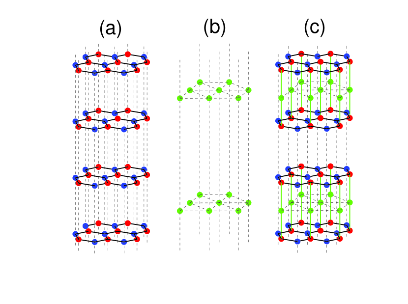
Figure 1: (a) The independent monolayer honeycomb lattice. (b) The adding triangular lattice. (c) The bilayer honeycomb lattice built with putting (a) and (b) together.

We consider a system of ultracold fermions confined in the bilayer honeycomb lattice. The honeycomb lattice consists of two sublattices denoted by $A$ and $B$. Then, the bilayer honeycomb lattice considered in our work is formed by coupling the $B$ sublattices of the two layers with tunneling and leaving the $A$ sublattices of the two layers uncoupled. One can create the bilayer honeycomb lattice in the following steps. First, one builds the monolayer honeycomb lattice as shown in Fig.1 (a) with three laser beams in the $x-y$ plane and two laser beams along the $z$ direction[21]. When the potential barrier of the optical lattice along the $z$ direction is high enough, the vertical tunneling between different planes is suppressed seriously, then every layer is an independent two-dimensional honeycomb lattice. Secondly, one makes the triangular lattice as shown in Fig.1 (b) with red-detuning laser fields[22]. Finally, to realize the bilayer honeycomb lattice, one can put the triangular lattice and the honeycomb lattice together as shown in Fig.1 (c). There exists an additional micro-trap between sublattices $B$ of every two layers in the honeycomb lattice. The additional micro-trap lowers the barrier between sublattices $B$ of these two layers in the honeycomb lattice, or links sublattices $B$ of these two layers in the honeycomb lattice as an intermediate point, so that sublattices $B$ of these two layers in the honeycomb lattice are coupled. Following this scheme, many independent bilayer honeycomb lattices can be achieved (see Fig.1 (c)), so we only need to investigated one of them. For convenience, we assume that the whole system is trapped in a two-dimensional box, which can be achieved by adding four blue detuning endcap beams at the edges of the optical lattice in $x-y$ plane[23]. With this box trap, the system can be considered to have the hard wall boundary condition approximately, so we can neglect the boundary effect in our discussion.

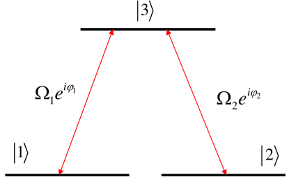
Figure 2: The light-atom interactions between fermionic atoms and two laser beams.

In this scheme, the ultracold atoms have a $\Lambda$-type three-level configuration, the states $|1\rangle$ and $|2\rangle$ are degenerate states, which are assumed to be different Zeeman states on the same hyperfine level, and $|3\rangle$ is an excited state. The ground state $|j\rangle$ with $j=1,2$ and the excited state $|3\rangle$ are coupled though two laser field with the corresponding Rabi frequencies $\Omega_{j}e^{i\varphi_{j}}$, respectively[18]. The schematic representation of this scheme is as shown in FIG. 2. The total Hamiltonian reads, $\hat{H}=\hat{H_{0}}+\hat{H_{1}}$. The non-perturbative Hamiltonian $\hat{H}_{0}$ is given by,

$$\hat{H}_{0}=\sum_{\alpha}\int d{\bf r}\hat{\Psi}^{\dagger}_{\alpha}({\bf r})\left[-{\hbar^{2}}\nabla^{2}/{2m}+V({\bf r})\right]\hat{\Psi}_{\alpha}({\bf r}),$$ (1)

and the light-atom interaction Hamiltonian $\hat{H}_{1}$ is given by,

$$\hat{H}_{1}=\int d{\bf r}\left[\Omega_{1}e^{i\varphi({\bf r})}\hat{\Psi}_{3}^{\dagger}({\bf r})\hat{\Psi}_{1}({\bf r})+\Omega_{2}\hat{\Psi}_{3}^{\dagger}({\bf r})\hat{\Psi}_{2}({\bf r})+{\rm H.c.}\right].$$ (2)

Diagonalizing the interaction Hamiltonian with the unitary transformation $S$,

$$S=\left(\begin{array}[]{ccc}\cos\theta&-\sin\theta e^{-i\varphi}&0\cr\frac{\sqrt{2}}{2}\sin\theta e^{i\varphi}&\frac{\sqrt{2}}{2}\cos\theta&-\frac{\sqrt{2}}{2}\cr\frac{\sqrt{2}}{2}\sin\theta e^{i\varphi}&\frac{\sqrt{2}}{2}\cos\theta&\frac{\sqrt{2}}{2}\end{array}\right),$$ (6)

yields three eigenstates $|\Phi_{1}\rangle$, $|\Phi_{2}\rangle$ and $|\Phi_{3}\rangle$, where $\tan\theta=|\Omega_{1}|/|\Omega_{2}|$ and $\varphi=\varphi_{1}-\varphi_{2}$ are both position-dependent variables. The corresponding eigenvalues are $E_{i}=(0,-\sqrt{|\Omega_{1}|^{2}+|\Omega_{2}|^{2}},\sqrt{|\Omega_{1}|^{2}+|\Omega_{2}|^{2}})$. The new field operators corresponding to the eigenstates are related with the old field operators as

$$\left(\begin{array}[]{c}\hat{\Phi}_{1}\\ \hat{\Phi}_{2}\\ \hat{\Phi}_{3}\end{array}\right)=S\left(\begin{array}[]{c}\hat{\Psi}_{1}\\ \hat{\Psi}_{2}\\ \hat{\Psi}_{3}\end{array}\right).$$ (13)

In the new bases, and under the adiabatic condition $\langle\Phi_{1}|\hat{H}_{0}|\Phi_{j}\rangle\ll|E_{i}-E_{j}|$ for $j=2,3$, we can apply the adiabatic condition and then neglect the populations of the states $|\Phi_{2}\rangle$ and $|\Phi_{3}\rangle$. Therefore, the effective Hamiltonian can be rewritten in the dark-state basis $|\Phi_{1}\rangle$ [16, 17, 18, 19, 20],

$$\hat{H}=\int d{\bf r}\hat{\Phi}_{1}^{\dagger}({\bf r})\left[\frac{1}{2m}(-i\hbar\nabla-{\bf{A}})^{2}+{V}_{eff}({\bf r})\right]\hat{\Phi}_{1}({\bf r}),$$ (14)

where ${\bf A}=-\hbar\sin^{2}\theta\nabla\varphi$ and $\hat{\cal H}\equiv\frac{1}{2m}(-i\hbar\nabla-{\bf{A}})^{2}+{V}_{eff}({\bf r})$ is the single particle Hamiltonian with $V_{eff}({\bf r})$ being the effective trap potential. Here $\bf A$ is the effective gauge potential associated with the artificial magnetic field ${\bf B}=\nabla\times{\bf A}$. In the practical case, we choose two counter-propagating Gaussian laser beams as $\Omega_{j}e^{i\varphi_{i}}=\Omega_{0}\exp[-(x-x_{j})^{2}/\sigma_{0}^{2}]\exp(-ik_{j}y)$ $(j=1,2)$, where the propagating wave vectors $k_{1}=-k_{2}=k_{0}/2$ and the center position $x_{1}=-x_{2}=\Delta x/2$ [18]. Then the effective trap potential is, [18]

$$V_{eff}({\bf r})=V({\bf r})+\frac{\hbar^{2}k_{0}^{2}}{2m}\frac{(1+1/4d^{2}k_{0}^{2})}{4\cosh^{2}(x/2d)},$$ (15)

and the effective vector gauge potential is

$${\bf A}=\frac{\hbar k_{0}}{1+e^{-x/d}}{\bf e}_{y},$$ (16)

with $d=\sigma_{0}^{2}/(4\Delta x)$. Straightforwardly, one can obtain the effective magnetic field, [18]

$${\bf B}=\frac{\hbar k_{0}}{4d\cosh^{2}(x/2d)}{\bf e}_{z}.$$ (17)

Practically, one may set $d\sim 1{\rm mm}$ and $-0.01{\rm mm}<x<0.01{\rm mm}$, so the condition $|x/d|\ll 1$ is satisfied. In this practical condition, the effective trap potential can approximately be written as

$$V_{eff}({\bf r})\approx V({\bf r})+\frac{\hbar^{2}k_{0}^{2}}{2m}\frac{(1+1/4d^{2}k_{0}^{2})}{4},$$ (18)

which has an additional constant term compared with the original external trap potential. This additional constant term does not change the geometrical structure of the original trap potential, so we can drop out it as a constant chemical potential term. The effective magnetic field can approximately be written as

$${\bf B}\approx{\bf B}^{(0)}+{\bf B}^{(2)}=\frac{\hbar k_{0}}{4d}{\bf e}_{z}-\frac{\hbar k_{0}}{4d}\frac{x^{2}}{8d^{2}}{\bf e}_{z}.$$ (19)

where the quadratic term can be neglected for $|B^{(2)}/B|<1.25\times 10^{-5}$. Thus, the effective magnetic field can be regarded as a homogeneous one in the regime considered in our scheme. For the typical parameter value $k_{0}\sim 2\times 10^{6}{\rm m}^{-1}$ and $d\sim 10^{-3}{\rm m}$, we obtain the magnitude of the effective magnetic field, $B\sim 3.3\times 10^{-25}{\rm J\cdot s\cdot m^{-2}}$.

3 The effective low energy Hamiltonian

Taking the tight-binding limit, we can superpose the Bloch states to get two sets of Wannier functions $w_{\alpha}^{A}({\bf r}-{\bf r}_{i})$ and $w_{\alpha}^{B}({\bf r}-{\bf r}_{j})$ with $\alpha=1,2$, which correspond to sublattices $A$ and $B$ of layer $\alpha$, respectively. In the presence of the effective gauge field we can expand the field operator in the lowest band Wannier functions as,

$$\hat{\Phi}_{1}({\bf r}) = \sum_{\alpha=1,2}\left[\sum_{i\in A}\hat{a}_{\alpha}({\bf r}_{i})e^{\frac{i}{\hbar}\int_{0}^{{\bf r}_{i}}{\bf A}\cdot d{\bf r}}w_{A}({\bf r}-{\bf r}_{i})\right.$$ (20)

$$\left.+\sum_{j\in B}\hat{b}_{\alpha}({\bf r}_{j})e^{\frac{i}{\hbar}\int_{0}^{{\bf r}_{j}}{\bf A}\cdot d{\bf r}}w_{B}({\bf r}-{\bf r}_{j})\right].$$

Substituting the above expression into Eq.(14), we can rewrite the Hamiltonian as $\hat{H}=\hat{H}_{0}+\hat{H}_{1}$ with [12],

$$\hat{H}_{0} = -t\sum_{\alpha}\sum_{{\bf r}_{i}\in A}\sum_{j=1,2,3}[\hat{a}_{\alpha}^{\dagger}({\bf r}_{i})\hat{b}_{\alpha}({\bf r}_{i}+{\bf s}_{j})e^{\frac{i}{\hbar}\int_{0}^{{\bf s}_{j}}{\bf A}\cdot d{\bf r}}+{\rm H.c.}],$$ (21)

and

$$\hat{H}_{1} = -t_{\perp}\sum_{{\bf r}_{i}\in A}[\hat{b}_{1}^{\dagger}({\bf r}_{i})\hat{b}_{2}({\bf r}_{i})+{\rm H.c.}],$$ (22)

where $t$ is the tunneling parameter with $t=-\int d{\bf r}w_{A}^{*}({\bf r}-{\bf r}_{i})\hat{\cal H}_{0}w_{B}({\bf r}-{\bf r}_{j})=-\int d{\bf r}w_{B}^{*}({\bf r}-{\bf r}_{j})\hat{\cal H}_{0}w_{A}({\bf r}-{\bf r}_{i})$; $t_{\perp}=-\int d{\bf r}w_{B_{2}}^{*}({\bf r}-{\bf r}_{i})\hat{\cal H}_{0}w_{B_{1}}({\bf r}-{\bf r}_{j})$; the energy shifts for sublattice A and B are $\epsilon_{A}=\int d{\bf r}w_{A}^{*}({\bf r}-{\bf r}_{i})\hat{\cal H}_{0}w_{A}({\bf r}-{\bf r}_{i})$ and $\epsilon_{B}=\int d{\bf r}w_{B}^{*}({\bf r}-{\bf r}_{j})\hat{\cal H}_{0}w_{B}({\bf r}-{\bf r}_{j})$ respectively, with $\hat{\cal H}_{0}\equiv-\frac{\hbar^{2}}{2m}\nabla^{2}+{V}_{eff}({\bf r})$. Here, for convenience, we can have dropped out a constant term in Hamiltonian (21). The three vector ${\bf s}_{j}$ in Eq.(21) are ${\bf s}_{1}=(0,-1)a,\ {\bf s}_{2}=\left({\sqrt{3}}/{2},{1}/{2}\right)a,\$ and ${\bf s}_{3}=\left(-{\sqrt{3}}/{2},{1}/{2}\right)a$, where $a$ is the lattice spacing. The three vector ${\bf s}_{i}(i=1,2,3)$ connect any site of sublattice $A$ to its nearest neighbor sites belonging to sublattice $B$ in every layer.

Here, we assume the condition $t_{\perp}\ll t$ being satisfied, so that we can consider Eq. (22) as a perturbation. We take the Fourier transformation to $\hat{a}({\bf r})$ and $\hat{b}({\bf r})$ as,

$$\hat{a}_{\alpha}({\bf k})=\sum_{{\bf r}_{i}\in A}e^{-i{\bf k}\cdot{\bf r}_{i}}\hat{a}_{\alpha}({\bf r}),$$ (23)

$$\hat{b}_{\alpha}({\bf k})=\sum_{{\bf r}_{i}\in B}e^{-i{\bf k}\cdot{\bf r}_{i}}\hat{b}_{\alpha}({\bf r}_{i}),$$ (24)

where ${\bf r}$ is the coordinate on $x-y$ plane. Substituting the above expressions into Eqs.(21) and (22), we obtain the following Hamiltonian,

$$\hat{H}_{0}=\sum_{\alpha}\sum_{k}[\xi({\bf k})\hat{a}_{\alpha}^{\dagger}({\bf k})\hat{b}_{\alpha}({\bf k})+\xi^{*}({\bf k})\hat{b}_{\alpha}^{\dagger}({\bf k})\hat{a}_{\alpha}({\bf k})],$$ (25)

$$\hat{H}_{1}=-t_{\perp}\sum_{{\bf k}}[\hat{b}_{1}({\bf k})^{\dagger}\hat{b}_{2}(k)+\hat{b}_{2}(k)^{\dagger}\hat{b}_{1}(k)],$$ (26)

where $\xi({\bf k})$ is the single-particle energy spectrum without interlayer tunneling and defined via $\xi({\bf k})=-t\sum_{j=1,2,3}e^{-i({\bf k}\cdot{\bf s}_{i}-\frac{1}{\hbar}\int_{0}^{{\bf s}_{j}}{\bf A}\cdot d{\bf r})}$. The energy spectrum contains two zero-energy points at ${\bf K}_{\pm}=\pm({4\pi}/{3\sqrt{3}a},0)$ around which it is linearized. Neglecting the coupling between the Fermi points ${\bf K}_{\pm}$, the total Hamiltonian $\hat{H}$ can be expand around the contact point ${\bf K}_{+}({\bf K}_{-})$ in coordinate space. Without loss of generality, we expand the total Hamiltonian around the contact point ${\bf K}_{+}$ as[12, 13],

$$\hat{H}=\int d^{2}r\hat{\psi}^{\dagger}({\bf r})\hat{\cal H}\hat{\psi}({\bf r}),$$ (27)

where the spinor $\hat{\psi}=({\hat{\psi}_{1}^{a}\ \ \hat{\psi}_{1}^{b}\ \ \hat{\psi}_{2}^{a}\ \ \hat{\psi}_{2}^{b}})^{T}$ for the Dirac point ${\bf K}_{+}$. Here, $\hat{\cal H}$ takes the $4\times 4$ matrix form,

$$\hat{\cal H}=\hbar\left(\begin{array}[]{cccc}0&v_{F}\hat{\pi}^{\dagger}&0&0\cr v_{F}\hat{\pi}&0&0&-t_{\perp}\cr 0&0&0&v_{F}\hat{\pi}^{\dagger}\cr 0&-t_{\perp}&v_{F}\hat{\pi}&0\end{array}\right),$$ (32)

where $\hat{\pi}=\hat{\pi}_{x}+i\hat{\pi}_{y}$ and $\hat{\pi}^{\dagger}=\hat{\pi}_{x}-i\hat{\pi}_{y}$, with $\hat{{\pi}}_{x}=\hat{p}_{x}-{A}_{x}/\hbar$ and $\hat{{\pi}}_{y}=\hat{p}_{y}-{A}_{y}/\hbar$, and $v_{F}=3at/2\hbar$ is the Fermi velocity. Here, $t_{\perp}\ll t$ is assumed. Eliminating the dimer state components $\hat{\psi}_{1}^{b}$ and $\hat{\psi}_{2}^{b}$, we can reach a two-component Hamiltonian describing effective hopping between the $A_{1}$-$A_{2}$ sites

$$\hat{\cal H}_{\rm eff}=\frac{\hbar^{2}}{2m}\left(\begin{array}[]{cc}0&\hat{\pi}^{\dagger}\hat{\pi}\cr\hat{\pi}^{\dagger}\hat{\pi}&0\end{array}\right),$$ (35)

where $m=t_{\perp}/2v_{F}^{2}$.

4 Energy bands

First, we consider the case without gauge fields, i.e. $\hat{{\pi}}_{x}=-i\partial_{x}$ and $\hat{{\pi}}_{y}=-i\partial_{y}$. The eigenfunctions of the Hamiltonian (35) are given by

$$f_{s{\bf k}}({\bf r})=\frac{1}{\sqrt{2}L}\exp(i{\bf k}\cdot{\bf r})\left(\begin{array}[]{c}s\cr 1\end{array}\right),$$ (38)

where $L^{2}$ is the area of the system, and $s$ denotes the conduction band with $s=+1$ and the valence band with $s=-1$. The corresponding eigenenergies are

$$E=\frac{s\hbar^{2}k^{2}}{2m},$$ (39)

where $k=\sqrt{k_{x}^{2}+k_{y}^{2}}$. This dispersion relation has parabolic form as shown in Fig.3. Here, the quasiparticles are still chiral like that in the monolayer system. The pseudospin vector ${\bf n}=(1,0)$ is a constant for any wave vector ${\bf k}$ in our work, while ${\bf n}=(\cos(2\phi),\sin(2\phi))$ for ${\bf k}=(k\cos\phi,k\sin\phi)$ in the bilayer graphene with Bernal stacking order as in References [14, 15]. Thus, in our bilayer honeycomb lattice configuration, the Berry phase $2\pi$ in the bilayer graphene with Bernal stacking order is absent.

5 Unconventional Landau levels

For the case with an effective magnetic field in the Landau gauge $(0,Bx,0)$, the eigenfunctions of the Hamiltonian (35) can be obtained as,

$$F_{nk_{y}}({\bf r}) = \frac{1}{\sqrt{2L}}\exp(ik_{y}y)\left(\begin{array}[]{c}\phi_{|n|}\cr{\rm sgn}(n)\phi_{|n|}\end{array}\right),$$ (42)

with ${\rm sgn}(n)=(1,0,-1)$ for $(n>0,n=0,n<0)$ respectively, for $n\neq 0$, and

$$F_{0k_{y}}({\bf r}) = \frac{1}{\sqrt{2L}}\exp(ik_{y}y)\left(\begin{array}[]{c}\phi_{0}\cr\pm\phi_{0}\end{array}\right),$$ (45)

for $n=0$. Here, $\phi_{n}$ are harmonic oscillator eigenstates as

$$\phi_{|n|}=\frac{1}{\sqrt{2^{|n|}|n|!\sqrt{\pi}u}}\exp\left[-\frac{1}{2}\left(\frac{x-u^{2}k}{u}\right)^{2}\right]H_{|n|}\left(\frac{x-u^{2}k}{u}\right),$$ (46)

where the quantum nubmer $n$ is an integer and $u=\sqrt{\hbar/B}$. The corresponding Landau energy levels are $E_{n}=n\hbar\omega_{c}$ with $n=\cdots,-2,-1,0,1,2,\cdots$ and $\omega_{c}=2v_{F}^{2}B/t_{\perp}$, which is shown in Fig.4. This spectrum has a linear form like the conventional Landau level spectrum. However, the quasiparticles are chiral in our scheme. The zero modes exist and the zero energy level is twofold degenerate compared to the non-zero energy levels.

To give a numerical evaluation, the typical values of the parameters can be taken as $t\sim 10^{-30}{\rm J}$, $t_{\perp}\sim 10^{-33}{\rm J}$, $a\sim 200{\rm nm}$, $B\sim 3.3\times 10^{-25}{\rm J\cdot s\cdot m^{-2}}$. We can then estimate the magnitude of the cyclotron frequency $\omega_{c}=5.7\times 10^{3}{\rm s^{-1}}$ and obtain the first gap of Landau level for the monolayer honeycomb lattice $\Delta\sim 6\times 10^{-31}{\rm J}$. The temperature required to keep atoms in the zeroth Landau level is $43\ {\rm nK}$.

6 Bragg spectroscopy

It is not easy to measure the Hall conductivity of cold fermionic atoms in the bilayer honeycomb lattice. However, an available method to detect the unconventional Landau levels of ultracold fermions on the bilayer honeycomb lattice is the Bragg spectroscopy[24], which is extensively used to probe the excitation spectrum in condensed matter physics. In the Bragg scattering, the atomic gas is exposed to two laser beams, with wavevectors ${\bf k}_{1}$ and ${\bf k}_{2}$ and a frequency difference $\omega$. The light-atom interaction Hamiltonian can be written as,

$$\hat{H}_{B}=\sum_{s_{1},s_{2},{\bf k},{\bf q}}\Omega_{B}e^{i{\bf q}\cdot{\bf r}}|f_{s_{2},{\bf k}+{\bf q}}\rangle\langle f_{s_{1},{\bf k}}|+{\rm H.c.},$$ (47)

where $s_{i}=1,2$. In our case, we consider the case of half filling, i.e., the bands with $n\leq 0$ are fully occupied and the bands with $n>0$ are empty. The half filling state can be prepared with the coherent filtering scheme proposed in Reference [25]. From the Fermi’s golden rule, we obtain the dynamic structure factor as follows,

$$S({\bf q},\omega) = \frac{1}{N\hbar^{2}\Omega^{2}}\sum_{\alpha}|\langle\phi_{\beta}^{(f)}|H_{B}|\phi_{\alpha}^{(i)}\rangle|^{2}$$ (48)

$$\times\delta(\hbar\omega-E_{\beta}+E_{\alpha})$$

where $N$ is the total number of atoms in the system; $\phi_{\alpha}^{(i)}$ denotes the initial state and $\phi_{\alpha}^{(f)}$ denotes the final state; $\alpha$ represents all quantum parameters of quantum state.

For simplicity, we assume that the direction of ${\bf q}$ is the same as the one of $y$ axis in the wavevector space, i.e. ${\bf q}=q{\bf e}_{y}$. Following the above formulae, we can straightforwardly evaluate the dynamic structure factor $S({\bf q},\omega)$. Fig.5(a) shows the dynamic structure factor $S({\bf q},\omega)$ as a function of $\omega$ for the case without an effective magnetic field. We can find that $S({\bf q},\omega)$ is zero when $\omega$ is under $\hbar^{2}q^{2}/2m$ and is finite constant for $\omega$ above $\hbar^{2}q^{2}/2m$. Fig.5 (b) shows the dynamic structure factor $S({\bf q},\omega)$ as a function of $\omega$ with $q=1.0\sqrt{B/\hbar}$ for the bilayer honeycomb lattice. Similarly, when a zero-level atom is excited to other states, the peaks are obtained at $\omega=(1,2,\cdots,n,\cdots)\Lambda^{2}t^{2}/\hbar t_{\perp}$ with $\Lambda=3a\sqrt{B/2\hbar}$, which are marked with red stars in FIG.3 (b). The distances between the neighbor peaks marked with red stars in Fig.3 (b) are identical.

7 Conclusion

In summary, we have proposed a scheme to investigate ultracold fermionic atoms in the bilayer honeycomb lattice for the cases without and with an effective magnetic field. The effective magnetic field can be built with optical techniques. For the case without an effective magnetic field, the dispersion relation has parabolic form and the quasiparticles are chiral. For the case with an effective magnetic field, there exist unconventional Landau levels that include a zero-mode level. We have calculated the dynamic structure factors for the two cases and proposed to detect them with the Bragg spectroscopy.

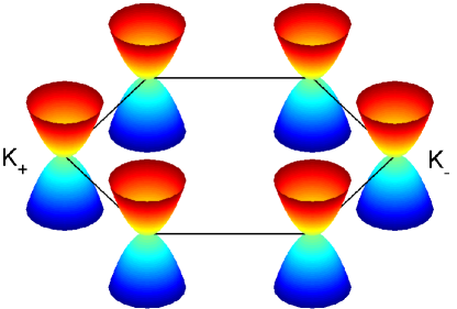
Figure 3: Energy bands of cold fermionic atoms in the bilayer honeycomb lattice without an effective magnetic field.

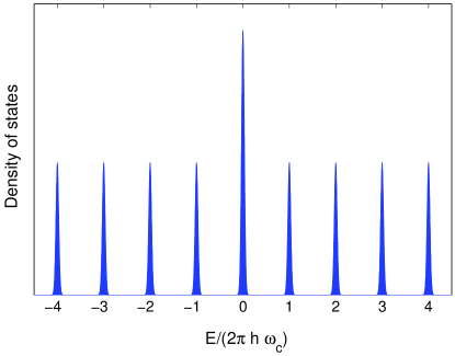
Figure 4: Landau levels of cold fermionic atoms in the bilayer honeycomb lattice with an effective magnetic field.

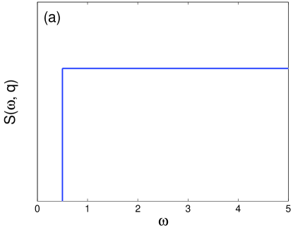
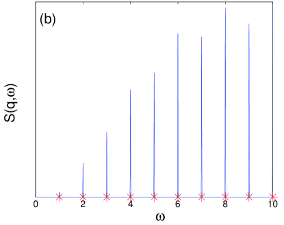
Figure 5: The dynamic structure factors $S(q,\omega)$ (not scaled) for cold atoms in the bilayer honeycomb lattice in the cases (a) without an effective magnetic field and (b) with an effective field. Here, $\omega$ is in units of $9at^{2}q^{2}/2\hbar t_{\perp}$ with $q=1.0\sqrt{B/\hbar}$.

References

- [1] Jaksch, D.; Bruder, C.; Cirac, J. I.; Gardiner, C. W.; Zoller, P. Phys. Rev. Lett. 1998, 81, 3108–3111.
- [2] Greiner, M.; Esslinger, T.; Mandel, O.; Hänsch, T. W.; Bloch, I. Nature 2002, 415, 39–44.
- [3] Lewenstein, M.; Sanpera, A.; Ahufinger, V.; Damski, B.; Sen, A.; Sen, U. Adv. Phys. 2007, 56, 243-379.
- [4] Rapp, Á.; Zaránd, G.; Honerkamp, C.; Hofstetter, W. Phys. Rev. Lett. 2007, 98, 160405-1–4.
- [5] Zhao, E.; Paramekanti, A. Phys. Rev. Lett. 2006, 97, 230404-1–4.
- [6] Zhu, S. L.; Wang, B.; Duan, L. M. Phys. Rev. Lett. 2007, 98, 260402-1–4.
- [7] Wu, C.; Bergman, D.; Balents, L.; Das Sarma, S. Phys. Rev. Lett. 2007, 99, 070401-1–4.
- [8] Zheng, Y.; Ando, T. Phys. Rev. B 2002, 65, 245420-1–11.
- [9] Novoselov, K. S.; Geim, A. K.; Morozov, S. V.; Jiang, D.; Katsnelson, M. I.; Grigorieva, I. V.; Dubonos S. V.; Firsov A. A. Nature 2005, 438, 197–200.
- [10] Li, G.; Andrei, E. Y. Nature Phys. 2007, 3, 623-627.
- [11] Zhang, Y.; Tan, Y. W.; Stormer, H. L.; Kim, P. Nature 2005, 438, 201–204.
- [12] Jackiw, R.; Pi, S. Y. Phys. Rev. Lett. 2007 ,98, 266402-1–4.
- [13] Hou, C. Y.; Chamon, C.; Mudry, C. Phys. Rev. Lett. 2007, 98, 186809-1–4.
- [14] McCann, E.; Fal’ko, V. I. Phys. Rev. Lett. 2006, 96, 086805-1–4.
- [15] McCann, E.; Abergel, D. S. L.; Fal’ko, V. I. Solid State Commun. 2007, 143, 110-115.
- [16] Juzeliūnas, G.; Öhberg, P.Phys. Rev. Lett. 2004, 93, 033602-1–4.
- [17] Juzeliūnas, G.; Öhberg, P.; Ruseckas, J.; Klein, A. Phys. Rev. A 2005, 71, 053614-1–9.
- [18] Juzeliūnas, G.; Ruseckas, J.; Öhberg, P.; Fleischhauer, M. Phys. Rev. A 2006, 73, 025602-1–4.
- [19] Liu, X. J.; Liu, X.; Kwek, L. C.; Oh, C. H. Phys. Rev. Lett. 2007, 98, 026602-1–4.
- [20] Zhu, S. L.; Fu, H.; Wu, C. J.; Zhang, S. C.; Duan, L. M. Phys. Rev. Lett. 2007, 97, 240401-1–4.
- [21] Duan, L. M.; Demler, E.; Lukin, M. D. Phys. Rev. Lett. 2003,91, 090402-1–4.
- [22] Grynberg, G.; Robilliard, C. Phys. Rep. 2001, 355, 335-451.
- [23] Meyrath, T. P.; Schreck, F; Hanssen, J. L.; Chuu, C. -S.; Raizen, M. G. Phys. Rev. A 2005, 71, 041604-1–4.
- [24] Stamper-Kurn, D. M.; Chikkatur, A. P.; Görlitz, A.; Inouye, S.; Gupta, S.; Pritchard, D. E.; Ketterle, W. Phys. Rev. Lett. 1999, 83, 2876-2879.
- [25] Rabl, P.; Daley, A. J.; Fedichev, P. O.; Cirac, J. I.; Zoller, P. Phys. Rev. Lett. 2003, 91, 110403-1–4.