On the mixing time of the 2D stochastic Ising model with “plus” boundary conditions at low temperature

Abstract.

We consider the Glauber dynamics for the 2D Ising model in a box of side $L$, at inverse temperature $\beta$ and random boundary conditions $\tau$ whose distribution ${\bf P}$ either stochastically dominates the extremal plus phase (hence the quotation marks in the title) or is stochastically dominated by the extremal minus phase. A particular case is when ${\bf P}$ is concentrated on the homogeneous configuration identically equal to $+$ (equal to $-$). For $\beta$ large enough we show that for any $\varepsilon>0$ there exists $c=c(\beta,\varepsilon)$ such that the corresponding mixing time $T_{\rm mix}$ satisfies $\lim_{L\to\infty}{\bf P}\left(T_{\rm mix}\geq\exp({cL^{\varepsilon}})\right)=0$. In the non-random case $\tau\equiv+$ (or $\tau\equiv-$), this implies that $T_{\rm mix}\leq\exp({cL^{\varepsilon}})$. The same bound holds when the boundary conditions are all $+$ on three sides and all $-$ on the remaining one. The result, although still very far from the expected Lifshitz behavior $T_{\rm mix}=O(L^{2})$, considerably improves upon the previous known estimates of the form $T_{\rm mix}\leq\exp({cL^{\frac{1}{2}+\varepsilon}})$. The techniques are based on induction over length scales, combined with a judicious use of the so-called “censoring inequality” of Y. Peres and P. Winkler, which in a sense allows us to guide the dynamics to its equilibrium measure. 2000 Mathematics Subject Classification: 60K35, 82C20 Keywords: Ising model, Mixing time, Phase coexistence, Glauber dynamics.

1. Introduction, model and main results

Glauber dynamics for classical spin systems has been extensively studied in the last fifteen years from various perspectives and across different areas like mathematical physics, probability theory and theoretical computer science. A variety of techniques have been introduced in order to analyze, on an increasing level of sophistication, the typical time scales of the relaxation process to the reversible Gibbs measure (see e.g. [17, 14] and the recent work on the cutoff phenomenon for the mean field Ising model [15]). These techniques have in general proved to be quite successful in the so-called one-phase region, corresponding to the case where the system has a unique Gibbs state. When instead the thermodynamic parameters of the system correspond to a point in the phase coexistence region, a whole class of new dynamical phenomena appear (coarsening, phase nucleation, motion of interfaces between different phases,…) whose mathematical analysis at a microscopic level is still quite far from being completed.

A good instance of the latter situation is represented by the Glauber dynamics for the usual $\pm 1$ Ising model at low temperature in the absence of an external magnetic field (see Section 1.2). When the system is analyzed in a finite box of side $L$ of the $d$-dimensional lattice ${\mathbb{Z}}^{d}$ with free boundary conditions, the relaxation to the Gibbs reversible measure occurs on a time scale exponentially large in the surface $L^{d-1}$ [27, 26] because of the energy barrier between the two stable phases of the system (see Section 1.3 for a more quantitative statement). When instead one of the two phases is selected by homogeneous boundary conditions, e.g. all pluses, then equilibration is believed to be much faster and it should occur on a polynomial (in $L$) time scale because of the shrinking of the big droplets of the opposite phase via motion by mean curvature under the influence of the boundary conditions. Unfortunately, establishing the above polynomial law in ${\mathbb{Z}}^{d}$ remains a kind of holy grail for the subject and the existing bounds of the form $\exp({c\sqrt{L\log(L)}})$ in $d=2$ [16, 12] and $\exp({cL^{d-2}\log(L)^{2}})$ in $d\geq 3$ [25] are very far from it.

It is worth mentioning that, always for the low-temperature Ising model but with the underlying graph $G$ different from ${\mathbb{Z}}^{d}$, it has been possible to carry out a quite detailed mathematical analysis. The first example is represented by the regular $d$-ary tree [18] and the second one by certain hyperbolic graphs [5]. In both cases one can show for example that the relaxation time or inverse spectral gap of the Glauber dynamics in a finite ball with all plus boundary conditions is uniformly bounded from above in the radius of the ball, a phenomenon that is believed to occur also in ${\mathbb{Z}}^{d}$ in large enough ($\geq 4$?) dimension $d$.

Moreover polynomial bounds on the mixing time, sometimes with optimal results, have been proved for some simplified models of the random evolution of the phase separation line between the plus and minus phase for the two-dimensional Ising model (see for instance [7] and [19]). The latter contribution, in particular, partly triggered the present work. There, in fact, the opportunities offered by the so-called Peres-Winkler censoring inequality [22] have been detailed in the very concrete and non-trivial case of the so-called Solid-on-Solid model.

Roughly speaking the censoring inequality (see Section 2.4) says that, when considering the Glauber dynamics for a monotone system like the Ising model on a finite graph and under certain conditions on the initial distribution, switching off (i.e., censoring) the spin flips in some part of the graph and for a certain amount of time can only increase the variation distance between the distribution of the chain at the final time $T$ and the equilibrium Gibbs measure. Therefore, if the censored dynamics is close to equilibrium at a certain time $T$, the same holds for the true (i.e. uncensored) one.

The fact that the choice of where and when to implement the censoring is completely arbitrary (provided that it is independent of the actual evolution of the chain) offers the possibility of (sort of) guiding the dynamics towards the stationary distribution through a sequence of local equilibrations in suitably chosen subsets of the graph. Of course the local equilibrium in each of the sub-graphs is conditioned to the random configuration reached by the dynamics outside it and therefore one is naturally led to consider the Ising model with random boundary conditions, a quite delicate topic because of the extreme sensitivity of the relaxation or mixing time to boundary conditions (see [1, 2, 3, 4] for several results in this direction, some of them quite surprising at first sight). Moreover it should also be clear that, in order for the guidance process to be successful, the distribution of the random boundary conditions at each stage of the censoring should be close to that provided by the stationary Gibbs distribution, a requirement that puts quite severe restrictions on the choice of the censoring scheduling.

The main contribution of this paper is a detailed implementation of this program for the two-dimensional, low-temperature, Ising model in a finite box with either homogeneous, i.e. all plus (all minus), boundary conditions or, more generally, random boundary conditions that are stochastically larger (stochastically smaller) than those distributed according to the plus (minus) phase.

In order to state precisely our results we need to define the model, fix some useful notation and recall some basic facts about the Ising model below the critical temperature.

1.1. The standard Ising model

Let $\Lambda$ be a generic finite subset of ${\mathbb{Z}}^{2}$. Each site $x$ in $\Lambda$ indexes a spin $\sigma_{x}$ which takes values $\pm 1$. The spin configurations $\{\sigma_{x}\}_{x\in\Lambda}$ have a statistical weight determined by the Hamiltonian

$$H^{\tau}(\sigma)=-\frac{1}{2}\sum_{x,y\in\Lambda\atop|x-y|=1}\sigma_{x}\sigma_{y}-\sum_{x\in\Lambda,y\in\Lambda^{c}\atop|x-y|=1}\sigma_{x}\tau_{y}\,,$$

where $\tau=\{\tau_{y}\}_{y\in\Lambda^{c}}$ are boundary conditions outside $\Lambda$.

The Gibbs measure associated to the spin system with boundary conditions $\tau$ is

$$\forall\sigma\in\Omega_{\Lambda}:=\{-1,+1\}^{\Lambda},\qquad\pi^{\tau}_{\Lambda}(\sigma)=\frac{1}{Z_{\beta,\Lambda}^{\tau}}\exp\left(-\beta H^{\tau}(\sigma)\right),$$

where $\beta$ is the inverse of the temperature ($\beta=\frac{1}{T}$) and $Z_{\beta,\Lambda}^{\tau}$ is the partition function. If the boundary conditions are uniformly equal to $+1$ (resp. $-1$), then the Gibbs measure will be denoted by $\pi_{\Lambda}^{+}$ (resp. $\pi_{\Lambda}^{-}$). If instead the boundary conditions are free (i.e. $\tau_{y}=0\ \forall y$) then the Gibbs measure will be denoted by $\pi_{\Lambda}^{f}$.

Remark 1.1.

Sometimes we will drop the superscript $\tau$ and the subscript $\Lambda$ from the notation of the Gibbs measure.

It is useful to recall a monotonicity property of the Gibbs measure that will play a key role in our analysis. One introduces a partial order on $\Omega_{\Lambda}$ by saying that $\sigma\leq\eta$ if $\sigma_{x}\leq\eta_{x}$ for all $x\in\Lambda$. A function $f:\Omega_{\Lambda}\mapsto\mathbb{R}$ is called monotone increasing (decreasing) if $\sigma\leq\eta$ implies $f(\sigma)\leq f(\eta)$ ($f(\sigma)\geq f(\eta)$). An event is called increasing (decreasing) if its characteristic function is increasing (decreasing). Given two probability measures $\mu$, $\nu$ on $\Omega_{\Lambda}$ we write $\mu\preceq\nu$ if $\mu(f)\leq\nu(f)$ for all increasing functions $f$ (with $\mu(f)$ we denote the expectation of $f$ with respect to $\mu$). In the following we will take advantage of the FKG inequalities [11] which state that

• if $\tau\leq\tau^{\prime}$, then $\pi_{\Lambda}^{\tau}\preceq\pi_{\Lambda}^{\tau^{\prime}}$

• if $f$ and $g$ are increasing then $\pi_{\Lambda}^{\tau}(fg)\geq\pi_{\Lambda}^{\tau}(f)\pi_{\Lambda}^{\tau}(g)$.

The phase transition regime occurs at low temperature and it is characterized by spontaneous magnetization in the thermodynamic limit. There is a critical value $\beta_{c}$ such that

$$\forall\beta>\beta_{c},\qquad\lim_{\Lambda\to{\mathbb{Z}}^{2}}\pi_{\Lambda}^{+}(\sigma_{0})=-\lim_{\Lambda\to{\mathbb{Z}}^{2}}\pi_{\Lambda}^{-}(\sigma_{0})=m_{\beta}>0\,.$$ (1.1)

Furthermore, in the thermodynamic limit the measures $\pi_{\Lambda}^{+}$ and $\pi_{\Lambda}^{-}$ converge (weakly) to two distinct Gibbs measures $\pi^{+}_{\infty}$ and $\pi^{-}_{\infty}$ which are measures on the space $\Omega_{\mathbb{Z}^{2}}=\{-1,+1\}^{{\mathbb{Z}}^{2}}$. Each of these measures represents a pure state.

The next step is to quantify the coexistence of the two pure states defined above. Let $\Lambda_{L}=\{-\lfloor L/2\rfloor,\dots,\lfloor L/2\rfloor\}^{2}$, let $\vec{n}$ be a vector in the unit circle ${\mathbb{S}}$ and $\phi_{\vec{n}}$ the angle it forms with $\vec{e}_{1}=(1,0)$ and finally let $\tau$ be the following mixed boundary conditions

$$\forall y\in\Lambda_{L}^{c},\qquad\tau_{y}=\begin{cases}+1,&\qquad\text{if}\quad\vec{n}\cdot y\;\geqslant\;0,\\ -1,&\qquad\text{if}\quad\vec{n}\cdot y<0.\end{cases}$$

The partition function with mixed boundary conditions is denoted by $Z_{\beta,L}^{\pm}(\vec{n})$ and the one with boundary conditions uniformly equal to $+1$ by $Z_{\beta,L}^{+}$.

Definition 1.2.

The surface tension in the direction orthogonal to $\vec{n}\in{\mathbb{S}}$ is an even and periodic function of $\phi_{\vec{n}}$ of period $\pi/2$, and for $-\pi/4\leq\phi_{\vec{n}}\leq\pi/4$ it is defined by

$$\tau_{\beta}(\vec{n})=\lim_{L\to\infty}\,-\frac{\cos(\phi_{\vec{n}})}{\beta L}\,\log\frac{Z_{\beta,L}^{\pm}(\vec{n})}{Z_{\beta,L}^{+}}\,.$$ (1.2)

We refer to [21] for a general derivation of the thermodynamic limit (1.2). With this definition, one result (among many others) concerning the coexistence of the two phases can be formulated as follows [23]. Let $m_{\Lambda_{L}}(\sigma)=\sum_{x\in\Lambda_{L}}\sigma_{x}$ be the total magnetization in the box $\Lambda_{L}$. Then

$$\lim_{L\to\infty}-\frac{1}{L}\log\left(\pi_{\Lambda_{L}}^{f}(\lfloor m_{\Lambda_{L}}/2\rfloor=0)\right)=\tau_{\beta}$$ (1.3)

where $\tau_{\beta}$ is the surface tension in the horizontal direction $\vec{e}_{1}$.

1.2. The Glauber dynamics

The stochastic dynamics we want to study, sometimes referred to as the heat-bath dynamics, is a continuous time Markov chain on $\Omega_{\Lambda}$, reversible w.r.t. the measure $\pi_{\Lambda}^{\tau}$, that can be described as follows. With rate one and for each vertex $x$, the spin $\sigma_{x}$ is refreshed by sampling a new value from the set $\{-1,+1\}$ according to the conditional Gibbs measure $\pi_{x}:=\pi_{\Lambda}^{\tau}(\cdot\thinspace|\thinspace\sigma_{y},\,y\neq x)$. It is easy to check that the heat-bath chain is characterized by the generator

$$(\mathcal{L}_{\Lambda}^{\tau}f)(\sigma)=\sum_{x\in\Lambda}\left[\pi_{x}(f)-f(\sigma)\right]$$ (1.4)

where $\pi_{x}(f)$ denotes the average of $f$ with respect to the conditional Gibbs measure $\pi_{x}$, which acts only on the variable $\sigma_{x}$. The Dirichlet form associated to $\mathcal{L}_{\Lambda}^{\tau}$ takes the form

$$\mathcal{E}_{\Lambda}^{\tau}(f,f)=\sum_{x\in\Lambda}\pi^{\tau}_{\Lambda}\bigl{(}\,\mathop{\rm Var}\nolimits_{x}(f)\,\bigr{)}$$

where $\mathop{\rm Var}\nolimits_{x}(f)$ denotes the variance with respect to $\pi_{x}$.

We will always denote by $\mu_{t}^{\sigma}$ the distribution of the chain at time $t$ when the starting point is $\sigma$. If $\sigma$ is either identically equal to $+1$ or $-1$ then we simply write $\mu_{t}^{+}$ or $\mu_{t}^{-}$. The boundary conditions $\tau$ are usually not explicitly spelled out for lightness of notation. Sometimes we write $\mu^{\sigma}_{\Lambda,t}$ when we wish to emphasize that we are looking at the evolution for a system enclosed in the domain $\Lambda$.

The Glauber dynamics with the heat-bath updating rule satisfies a particularly useful monotonicity property. It is possible to construct on the same probability space (the one built from the independent Poisson clocks attached to each vertex and from the independent coin tosses associated to each ring) a Markov chain $\{\eta_{t}^{\sigma,\tau}\}_{t\geq 0}$, $(\sigma,\tau)\in\Omega_{\Lambda}\times\Omega_{\Lambda^{c}}$, such that

• for each $\tau\in\Omega_{\Lambda^{c}}$ and $\sigma\in\Omega_{\Lambda}$ the coordinate process $(\eta_{t}^{\sigma,\tau})_{t\geq 0}$ is a version of the Glauber chain started from $\sigma$ with boundary conditions $\tau$;

• for any $t\geq 0$, $\eta_{t}^{\sigma,\tau}\leq\eta_{t}^{\sigma^{\prime},\tau^{\prime}}$ whenever $\sigma\leq\sigma^{\prime}$ and $\tau\leq\tau^{\prime}$.

It is possible to extend the above definition of the generator $\mathcal{L}_{\Lambda}^{\tau}$ directly to the whole lattice ${\mathbb{Z}}^{2}$ and get a well defined Markov process on $\Omega_{{\mathbb{Z}}^{2}}$ (see e.g. [13]). The latter will be referred to as the infinite volume Glauber dynamics, with generator denoted by $\mathcal{L}$.

Two key quantities measure the speed of relaxation to equilibrium of the Glauber dynamics. The first one is the relaxation time $T_{\rm relax}$.

Definition 1.3.

$T_{\rm relax}$ is the best constant $C$ in the Poincaré inequality

$$\mathop{\rm Var}\nolimits_{\Lambda}^{\tau}(f):=\mathop{\rm Var}\nolimits_{\pi_{\Lambda}^{\tau}}(f)\leq C\mathcal{E}_{\Lambda}^{\tau}(f,f),\qquad\forall\;f:\Omega_{\Lambda}\mapsto{\mathbb{R}}.$$ (1.5)

In particular, for any $f:\Omega_{\Lambda}\mapsto{\mathbb{R}}$, it follows that

$$\mathop{\rm Var}\nolimits_{\Lambda}^{\tau}\left(e^{t\mathcal{L}_{\Lambda}^{\tau}}f\right)^{1/2}\leq e^{-t/T_{\rm relax}}\mathop{\rm Var}\nolimits_{\Lambda}^{\tau}\left(f\right)^{1/2}.$$ (1.6)

We will write $\mathop{\rm gap}\nolimits:=\mathop{\rm gap}\nolimits^{\tau}_{\Lambda}$ for the inverse of $T_{\rm relax}$.

Another relevant quantity is the mixing time which is defined as follows. Recall that the total variation distance between two measures $\mu,\nu$ on a finite probability space $\Omega$ is defined as

$$\|\mu-\nu\|:=\frac{1}{2}\sum_{\sigma\in\Omega}|\mu(\sigma)-\nu(\sigma)|.$$ (1.7)

Definition 1.4.

For any $\epsilon\in(0,1)$, we define

$$T_{\rm mix}(\epsilon):=\inf\{t>0:\sup_{\sigma}\|\mu_{t}^{\sigma}-\pi_{\Lambda}^{\tau}\|\leq\epsilon\}.$$ (1.8)

When $\epsilon=1/(2e)$ we will simply write $T_{\rm mix}$.

With this definition it follows in particular that (see e.g. [14])

$$\sup_{\sigma}\|\mu_{t}^{\sigma}-\pi_{\Lambda}^{\tau}\|\leq\left(2\epsilon\right)^{\lfloor t/T_{\rm mix}(\epsilon)\rfloor}\quad\forall t\geq 0.$$ (1.9)

As it is well known (see e.g. [14]) the following bounds between $T_{\rm relax}$ and $T_{\rm mix}$ hold:

$$T_{\rm relax}\leq T_{\rm mix}\leq\log\left(\frac{2e}{\pi^{*}}\right)T_{\rm relax}$$ (1.10)

where $\pi^{*}=\min_{\sigma}\pi_{\Lambda}^{\tau}(\sigma)$. Notice that $\pi^{*}\geq e^{-c|\Lambda|}$ for some constant $c=c(\beta)$ and therefore the two quantities differ at most by const$\times$volume.

Another definition we will often need is the following:

Definition 1.5.

Let $\mu,\nu$ be measures on $\Omega_{\Lambda}$, let $\sigma\in\Omega_{L}$ and $V\subset\Lambda$. Then, $\|\mu-\nu\|_{V}$ denotes the variation distance between the marginals of $\mu$ and $\nu$ on $\Omega_{V}$, and $\sigma_{V}$ the restriction of $\sigma$ to $V$.

1.3. Main results

Our main result considerably improves upon the existing upper bound on the mixing time (and therefore also on the relaxation time) when $\Lambda$ is a square box and the boundary conditions $\tau$ are homogeneous i.e. either all plus or all minus. As a by-product we also get a new bound on the time auto-correlation function of, e.g., the spin at the origin for the infinite volume Glauber dynamics started from the plus phase $\pi^{+}_{\infty}$. Before stating the results we quickly review what was known so far. In what follows $\Lambda_{L}$ will always be a $L\times L$ box.

When the boundary conditions are free, a simple bottleneck argument proves that

$$T_{\rm relax}\geq\frac{1}{L^{2}}\left(\pi_{\Lambda_{L}}^{f}(\lfloor m_{\Lambda_{L}}/2\rfloor=0)\right)^{-1}$$

so that (recall (1.3))

$$\lim_{L\to\infty}\frac{1}{L}\log(T_{\rm relax})\geq\tau_{\beta}.$$

In [16] such a result was improved to an equality for large enough values of $\beta$ and in [8] for any $\beta>\beta_{c}$.

Quite different is the situation for homogeneous boundary conditions, e.g. all plus, for which the bottleneck between the two phases is removed by the boundary conditions and the relaxation process should occur on a much shorter time scale. In this case one expects a polynomial growth of both $T_{\rm relax}$ and $T_{\rm mix}$ of the form

$$T_{\rm relax}\approx L,\qquad T_{\rm mix}\approx L^{2}.$$

The reason behind the difference in the power of $L$ of the two growths seems to be quite subtle and largely not yet understood at the mathematical level. The only rigorous results in this direction are those obtained in [6] where, apart from logarithmic corrections, the appropriate lower bounds on $T_{\rm relax}$ and $T_{\rm mix}$ have been established by means of quite subtle test functions combined with the whole machinery of the Wulff construction.

As far as upper bounds are concerned, they proved to be quite hard to obtain and the available results are still quite poor. In the case of homogeneous boundary conditions it was first shown in [16] that, for $\beta$ large enough and any $\varepsilon>0$,

$$T_{\rm relax}\leq\exp\left({cL^{1/2+\varepsilon}}\right)$$

for a suitable constant $c$ depending on $\varepsilon$ and $\beta$. Later such a bound was improved to $\exp({c\sqrt{L\log L}})$ in [12]. When the inverse temperature $\beta$ is just above the critical value, the only available result is much weaker (see [8]) and of the form

$$\lim_{L\to\infty}\frac{1}{L}\log(T_{\rm relax})=0.$$

Finally when $f(\sigma)=\sigma_{0}$ the above bounds combined with some simple monotonicity arguments prove that, for any $\alpha>0$,

$$\mathop{\rm Var}\nolimits^{+}_{\infty}\left(e^{t\mathcal{L}}f\right)\leq c/t^{\alpha}$$

(where $\mathop{\rm Var}\nolimits^{+}_{\infty}$ denotes the variance w.r.t. the plus phase $\pi^{+}_{\infty}$) while the expected behavior is $O(e^{-\sqrt{t}})$, see [10].

We are now in a position to state our main results.

Theorem 1.6.

Let $\beta$ be large enough and let $L$ belong to the sequence $\{2^{n}-1\}_{n\in\mathbb{N}}$.

1. If the boundary conditions (b.c.) $\tau$ are sampled from a law ${\bf P}$ which either stochastically dominates the pure phase $\pi^{+}_{\infty}$ or is stochastically dominated by $\pi^{-}_{\infty}$ (see Section 2.2), there exists $c=c(\beta,\varepsilon)$ (independent of ${\bf P}$) such that

   $${\bf E}\|\mu^{\pm}_{t_{L}}-\pi^{\tau}\|\leq\exp\left(-cL^{\varepsilon^{2}/16}\right),$$ (1.11)

   where $t_{L}=\exp(cL^{\varepsilon})$. In particular,

   $${\bf P}\left(T_{\rm mix}\geq t_{L}\right)\leq\exp\left(-cL^{\varepsilon^{2}/16}\right).$$ (1.12)

2. The estimates (1.11)-(1.12) hold also if ${\bf P}$ is stochastically dominated by $\pi^{-}_{\infty}$ on one side of $\Lambda_{L}$, and stochastically dominates $\pi^{+}_{\infty}$ on the union of the other three sides. Similarly if the role of $+$ and $-$ is reversed.

The most natural consequence of the above result is

Corollary 1.7.

Let $\beta$ be large enough and let $L$ belong to the sequence $\{2^{n}-1\}_{n\in\mathbb{N}}$. Consider the square $\Lambda_{L}$ with b.c. $\tau\equiv+$. For every $\varepsilon>0$ there exists $c=c(\beta,\varepsilon)<\infty$ such that

$$T_{\rm mix}\leq e^{cL^{\varepsilon}}.$$ (1.13)

The same bound holds if the boundary conditions are $+$ on three sides and $-$ on the remaining one. Similarly if $+$ is replaced by $-$.

Remark 1.8.

(i) In the proof of Theorem 1.6 and of Corollary 1.10 below, we need at some point some key equilibrium estimates which are proved in the appendix via standard cluster expansion techniques for values of $\beta$ large enough. However, we expect those bounds to hold for every $\beta>\beta_{c}$. Since this is the only part of the proof where the value of $\beta$ comes into play, we expect Theorem 1.6 and Corollary 1.10 to hold for any $\beta>\beta_{c}$. Let us also point out that, while we restrict for simplicity to the nearest-neighbor Ising model, we believe that our techniques can be generalized without conceptual difficulties to ferromagnetic Ising models with finite-range interactions. In particular, cluster expansion results for large $\beta$ are known to hold also in this more general situation.

(ii) The restriction that $L$ belongs to the sequence $\{2^{n}-1\}_{n\in\mathbb{N}}$ is purely technical and it is a consequence of the iterative procedure we use. It would not be difficult to eliminate this restriction by somewhat modifying our iteration below (see Remark 3.12 at the end of the proof of Theorem 3.2), but we have decided not to do this, in order to keep the presentation as simple as possible.

(iii) The above results have been stated for the heat-bath dynamics but they actually apply to any other single site Glauber dynamics (e.g. the Metropolis chain) with jump rates uniformly positive (e.g. greater than $\delta>0$) as can be seen via standard comparison techniques [17]. More precisely, if $\hat{T}_{\rm mix}$ and $\hat{T}_{\rm relax}$ denote the mixing and relaxation times of the new chain, then there exist constants $c,c^{\prime}$ depending on $\delta,\beta$ such that $\hat{T}_{\rm mix}\leq c|\Lambda|\hat{T}_{\rm relax}\leq c^{\prime}|\Lambda|T_{\rm relax}\leq c^{\prime}|\Lambda|T_{\rm mix}$; the results we are after then follow since $|\Lambda|$ represents a polynomial correction which is irrelevant in our case.

(iv) Notice that in some sense our result (1.12) is not so far from optimality. Indeed, consider the distribution ${\bf P}$ such that $\tau=+$ except for the boundary sites which are at distance at most $L^{\varepsilon}$ from one of the corners of the box, where $\tau$ is sampled from $\pi^{+}_{\infty}$. Clearly ${\bf P}$ stochastically dominates $\pi^{+}_{\infty}$. Then, with ${\bf P}$-probability $\exp(-cL^{\varepsilon})$, $\tau=-$ around the corners and, thanks to the results of [1], $T_{mix}\geq\exp(cL^{\varepsilon})$.

1.4. Applications

It is intuitive that if the b.c. are all $+$ (all $-$) and we start from the all $+$ (all $-$) configuration, equilibration will be much quicker. Indeed, we have the following

Corollary 1.9.

Let $\beta$ be large enough and $\tau\equiv+$. For every $\varepsilon>0$ there exists $c=c(\beta,\varepsilon)>0$ such that

$$\lim_{L\to\infty}\|\mu^{+}_{t_{1}}-\pi^{\tau}\|=0,$$ (1.14)

where $t_{1}:=\exp(c(\log L)^{\varepsilon})$ . By a global spin flip the same results holds if $+$ is replaced by $-$.

Finally, here is the result about the decay of time auto-correlations for the infinite-volume dynamics in a pure phase:

Corollary 1.10.

Let $\beta$ be large, let $f(\sigma)=\sigma_{0}$ and let $\rho(t)\equiv\mathop{\rm Var}\nolimits^{+}_{\infty}\left(e^{t\mathcal{L}}f\right)$ be the time auto-correlation of the spin at the origin in the plus phase $\pi^{+}_{\infty}$. Then for any $\varepsilon>0$ there exists a constant $c=c(\beta,\varepsilon)$ such that

$$\rho(t)\leq c\,e^{-(1/c)(\log t)^{1/\varepsilon}}.$$ (1.15)

2. Auxiliary definitions and results

In this section we collect some more detailed notation that will be needed during the proof of the main results, together with certain additional auxiliary results that will play a key role in our analysis.

2.1. Geometrical definitions

Figure 1. The rectangle $\Lambda$ and its enlargement $E_{L}(\Lambda)$

The boundary of a finite subset $\Lambda\subset\mathbb{Z}^{2}$, in the sequel denoted by $\partial\Lambda$, consists of those sites in ${\mathbb{Z}}^{2}\setminus\Lambda$ at unit distance from $\Lambda$. Given a rectangle $\Lambda\subset\mathbb{Z}^{2}$ and $L\in\mathbb{N}$, we denote by $E_{L}(\Lambda)$ the enlarged rectangle obtained from $\Lambda$ by shifting by $L$ units the Northern boundary upwards, the Eastern boundary eastward and the Western boundary westward (see Figure 1).

Given $\varepsilon>0$ (to be thought of as very small) and $L\in\mathbb{N}$ we let

$$R^{\varepsilon}_{L}=\{(i,j)\in{\mathbb{Z}}^{2}:\ 1\leq i\leq L,\,1\leq j\leq\lceil L^{\frac{1}{2}+\varepsilon}\rceil\}.$$

Similarly we define the rectangle $Q^{\varepsilon}_{L}$, the only difference being that the vertical sides contain now $\lceil(2L+1)^{\frac{1}{2}+\varepsilon}\rceil$ sites.

Notation warning. In the sequel we will often remove the superscript $\varepsilon$ from our notation of the various rectangles involved since it is a (small) parameter that we imagine given once and for all.

2.2. Boundary conditions

A boundary condition $\tau$ for a given domain (typically, a rectangle) is an assignment of values $\pm 1$ to each spin on the boundary of the domain under consideration.

Definition 2.1.

A distribution ${\bf P}$ of b.c. for a rectangle $R$ (which will be $R_{L}$, $Q_{L}$ or a rectangle obtained by translating one of them by a vector $v\in\mathbb{Z}^{2}$) is said to belong to $\mathcal{D}(R)$ if its marginal on the union of North, East and West borders of $R$ is stochastically dominated by (the marginal of) the minus phase $\pi^{-}_{\infty}$ of the infinite system, while the marginal on the South border of $R$ dominates the (marginal of the) infinite plus phase $\pi^{+}_{\infty}$.

The most natural example is to take ${\bf P}$ concentrated on the boundary conditions $\tau$ given by $\tau\equiv-$ on the North, East and West borders, and $\tau\equiv+$ on the South border. In that case we will sometimes write $\pi_{R}^{-,-,+,-}$ for the equilibrium measure in $R$, where we agree to order the sides of the border clockwise starting from the Northern one.

2.3. The inductive statements

Here we define two inductive statements that will be proved later by a “halving the scale” technique.

Definition 2.2.

For any given $L\in\mathbb{N},\delta>0,t>0$ consider the system in $R_{L}$, with boundary condition $\tau$ chosen from some distribution $\bf P$. We say that $\mathcal{A}(L,t,\delta)$ holds if

$${\bf E}\|\mu^{\pm}_{t}-\pi^{\tau}\|\leq\delta$$ (2.1)

for every ${\bf P}\in\mathcal{D}(R_{L})$.

The statement $\mathcal{B}(L,t,\delta)$ is defined similarly, the only difference being that the rectangle $R_{L}$ is replaced by $Q_{L}$ (in particular, ${\bf P}$ is required to belong to $\mathcal{D}(Q_{L})$).

2.4. Censoring inequalities

In this section, we consider the Glauber dynamics in a generic finite domain $\Lambda\subset\mathbb{Z}^{2}$, not necessarily a rectangle. The boundary conditions $\tau$ are not specified, because the results are independent of it.

A fundamental role in our work is played by the censoring inequality proved recently by Y. Peres and P. Winkler: this says, roughly speaking, that removing (deterministically) some updates from the dynamics can only slow down equilibration, if the initial configuration is the maximal (or minimal) one.

First of all we need a simple but useful lemma:

Lemma 2.3.

[22, Lemma 16.7] Let $\pi,\mu,\nu$ be laws on a finite, partially ordered probability space. If $\nu\preceq\mu$ and $\nu/\pi$ is increasing, i.e.

$$\frac{\nu(\sigma)}{\pi(\sigma)}\geq\frac{\nu(\eta)}{\pi(\eta)}$$ (2.2)

whenever $\sigma\geq\eta$, then

$$\|\nu-\pi\|\leq\|\mu-\pi\|.$$ (2.3)

The result of Peres-Winkler can be stated as follows:

Theorem 2.4.

[22, Theorem 16.5] Let $m\in\mathbb{N}$, $\underline{v}:=(v_{1},\ldots,v_{m})$ a sequence of sites in $\Lambda$, and let $\underline{v}^{\prime}$ be a sub-sequence of $\underline{v}$. Let $\mu_{0}$ be a law on $\Omega_{\Lambda}$ such that $\mu_{0}/\pi$ is increasing. Denote by $\mu_{\underline{v}}$ the law obtained starting from $\mu_{0}$ and performing heat-bath updates at the ordered sequence of sites $\underline{v}$. Similarly for $\mu_{\underline{v}^{\prime}}$. Then,

$$\|\mu_{\underline{v}}-\pi\|\leq\|\mu_{\underline{v}^{\prime}}-\pi\|$$ (2.4)

and $\mu_{\underline{v}}\preceq\mu_{\underline{v}^{\prime}}$. Moreover, $\mu_{\underline{v}}/\pi$ and $\mu_{\underline{v}^{\prime}}/\pi$ are increasing.

It is easy to see that, if $\mu_{0}/\pi$ is instead decreasing, (2.4) still holds, while the other statements become $\mu_{\underline{v}^{\prime}}\preceq\mu_{\underline{v}}$ and $\mu_{\underline{v}}/\pi$, $\mu_{\underline{v}^{\prime}}/\pi$ decreasing.

Here, “performing a heat-bath update at a given site $v\in\Lambda$” simply means freezing the configuration outside $v$ and extracting $\sigma_{v}$ from the equilibrium distribution conditioned on the configuration outside $v$.

Theorem 2.4 is proved in [22] in the particular case where $\mu_{0}$ is the measure concentrated at the all $+$ configuration, but the proof of the above generalized statement is essentially identical. Let us emphasize that such result is not specific of the Ising model but requires in an essential way monotonicity of the dynamics.

From Lemma 2.3 and Theorem 2.4 we easily extract the continuous-time censoring inequality we need:

Theorem 2.5.

Let $n\in\mathbb{N}$, $0\equiv t_{0}<t_{1}<\ldots t_{n}\equiv T$ and $\Lambda_{i}\subset\Lambda,i=1,\ldots,n$. Let $\mu_{0}$ be a law on $\Omega_{\Lambda}$ such that $\mu_{0}/\pi$ is increasing. Let $\mu_{T}$ be the law at time $T$ of the continuous-time, heat-bath dynamics in $\Lambda$, started from $\mu_{0}$ at time zero. Also, let $\mu^{\prime}_{T}$ be the law at time $T$ of the modified dynamics which again starts from $\mu_{0}$ at time zero, and which is obtained from the above continuous time, heat-bath dynamics by keeping only the updates in $\Lambda_{i}$ in the time interval $[t_{i-1},t_{i})$ for $i=1,\ldots,n$. Then,

$$\|\mu_{T}-\pi\|\leq\|\mu^{\prime}_{T}-\pi\|,$$ (2.5)

and $\mu_{T}\preceq\mu^{\prime}_{T}$; moreover, $\frac{\mu_{T}}{\pi}$, $\frac{\mu^{\prime}_{T}}{\pi}$ are both increasing.

Needless to say, if instead $\mu_{0}/\pi$ is decreasing then all inequalities except (2.5) are reversed.

Proof. Let $m$ be the (random) number of Poisson clocks which ring during the time interval $[0,T)$, and denote by $s_{i}$ and $v_{i}\in\Lambda,i\leq m$ the times and sites where they ring. We order the times as $s_{i}<s_{i+1}$ and of course $v_{i}$ are IID and chosen uniformly in $\Lambda$. Define then $w:=((v_{1},s_{1}),\ldots,(v_{m},s_{m}))$ and let $\mu_{w}$ be obtained from $\mu_{0}$ performing single-site heat-bath updates at sites $v_{1},v_{2},\ldots,v_{m}$ (in this order). Analogously, let $w^{\prime}$ be obtained by $w$ by removing all pairs $(v_{j},s_{j})$ such that $v_{j}\notin\Lambda_{k}$ where $k$ is such that $s_{j}\in[t_{k-1},t_{k})$, and $\mu_{w^{\prime}}$ be defined in the obvious way. For any realization of $w$ one has from Theorem 2.4 that $\mu_{w}\preceq\mu_{w^{\prime}}$ and that both $\mu_{w}/\pi$ and $\mu_{w^{\prime}}/\pi$ are increasing. Since $\mu_{T}$ (respectively $\mu^{\prime}_{T}$) is just the average over $w$ of $\mu_{w}$ (resp. of $\mu_{w^{\prime}}$), one obtains all the claims of the theorem (except (2.5)) by linearity. Inequality (2.5) comes simply from $\mu_{T}\preceq\mu^{\prime}_{T}$, plus Lemma 2.3 and the fact that $\mu_{T}/\pi$ is increasing. ∎

We will need at various instances the following easy consequences of the above facts.

Corollary 2.6.

Let $t>0$ and assume that $\mu_{0}/\pi$ is increasing. Denote by $\mu_{t}$ the evolution started from $\mu_{t=0}=\mu_{0}$, and by $\mu_{t}^{+}$ the one started from the maximal configuration $+$. Then

$$\|\mu_{t}-\pi\|\leq\|\mu_{t}^{+}-\pi\|.$$ (2.6)

Proof.

We know from Theorem 2.5 that $\mu_{t}/\pi$ is increasing. Moreover, by monotonicity of the dynamics $\mu_{t}\preceq\mu_{t}^{+}$. The claim then follows from Lemma 2.3. ∎

Corollary 2.7.

Let $\gamma(t)=\max\left(\|\mu^{+}_{t}-\pi\|,\|\mu^{-}_{t}-\pi\|\right)$. Then

$$\gamma(t+s)\leq 4\gamma(t)\gamma(s)\qquad\forall t,s\geq 0.$$

Proof.

Notice that $\|\mu^{+}_{t+s}-\pi\|=\mu^{+}_{t+s}(A)-\pi(A)$ where $A=\{\sigma:\ \mu^{+}_{t+s}(\sigma)\geq\pi(\sigma)\}$. Because of Theorem 2.5 the event $A$ is increasing so that $f:={1\mskip-5.0mu{\rm I}}_{A}-\pi(A)$ is an increasing function (and of course $\pi(f)=0$). Thus

$$\|\mu^{+}_{t+s}-\pi\| = \mu^{+}_{t+s}(A)-\pi(A)$$

$$= \mu^{+}_{t}\left(\mu^{\sigma}_{s}(f)\right)$$

$$= \mu^{+}_{t}\left(\mu_{s}^{\sigma}(f)\right)-\pi\left(\mu_{s}^{\sigma}(f)\right)$$

$$\leq 2\gamma(t)\sup_{\sigma}|\mu_{s}^{\sigma}(f)|$$

$$\leq 2\gamma(t)\max\{|\mu_{s}^{+}(f)|,|\mu_{s}^{-}(f)|\}$$

$$\leq 4\gamma(t)\gamma(s).$$

Similarly for $\mu^{-}$. ∎

2.5. Perturbation of the boundary conditions and mixing time

Consider a finite set $\Lambda$ and two boundary conditions $\tau,\hat{\tau}$. Let $T_{\rm mix}$ and $\hat{T}_{\rm mix}$ be the associated mixing times for the Glauber chain in $\Lambda$ with b.c. $\tau$ and $\hat{\tau}$, respectively. Let $M=\max\{\|\frac{\pi^{\tau}}{\pi^{\hat{\tau}}}\|_{\infty},\|\frac{\pi^{\hat{\tau}}}{\pi^{\tau}}\|_{\infty}\}$.

Lemma 2.8.

There exists a constant $c$ independent of $\Lambda,\tau,\hat{\tau}$ such that

$$T_{\rm mix}\leq cM^{3}|\Lambda|\hat{T}_{\rm mix}.$$ (2.7)

Proof.

Thanks to (1.10) and to the variational characterization of the relaxation time we get

$$T_{\rm mix}\leq c|\Lambda|T_{\rm relax}\leq c|\Lambda|M^{3}\hat{T}_{\rm relax}\leq c|\Lambda|M^{3}\hat{T}_{\rm mix}$$

where the third power of $M$ comes from expressing the Dirichlet form, the variance and the local variances w.r.t. $\pi^{\tau}$ in terms of those w.r.t. $\pi^{\hat{\tau}}$. ∎

Let now $\Delta\subset\partial\Lambda$, let $\tau_{\Delta}$ be some configuration in $\Omega_{\Delta}$, let ${\bf P}$ be some distribution over the boundary conditions on $\partial\Lambda$ and let ${\bf P}^{\Delta}$ be the distribution which assigns probability zero to b.c. $\tau$ not identically equal to $\tau_{\Delta}$ on $\Delta$ and whose marginal on $\partial\Lambda\setminus\Delta$ coincides with the same marginal of ${\bf P}$. Notice that we can sample from ${\bf P}^{\Delta}$ by first sampling from ${\bf P}$ and then changing (if necessary) to $\tau_{\Delta}$ the spins of $\tau$ in $\Delta$. If the pair so obtained is denoted by $(\tau,\hat{\tau})$ then the corresponding constant $M$ satisfies $M\leq M_{\Delta}:=e^{8\beta|\Delta|}$.

Let $d^{\pm}(t)=\|\mu_{t}^{\pm}-\pi^{\tau}\|$ so that $\gamma(t)=\max\{d^{+}(t),d^{-}(t)\}$. Similarly for $\hat{d}^{\,\pm}(t),\hat{\gamma}(t)$.

Lemma 2.9.

With the above notation

$${\bf E}\left(\gamma(t)\right)\leq e^{-M_{\Delta}}+8{\bf E}\left(\hat{\gamma}(\hat{t})\right)$$

where $\hat{t}=t/(c|\Lambda|^{2}M_{\Delta}^{4})$.

Proof.

Thanks to (2.7) and (1.9),

$${\bf E}\left(\gamma(t)\right)\leq e^{-M_{\Delta}}+{\bf P}\left(T_{\rm mix}\geq t/M_{\Delta}\right)\leq e^{-M_{\Delta}}+{\bf P}\left(\hat{T}_{\rm mix}\geq t/(c|\Lambda|M_{\Delta}^{4})\right)$$

$$=e^{-M_{\Delta}}+{\bf P}\left(\hat{T}_{\rm mix}\geq|\Lambda|\hat{t}\right).$$

Notice that, for any $s\geq 0$, $\hat{T}_{\rm mix}\geq s$ implies that there exists some starting configuration $\sigma$ for which the variation distance of its distribution at time $s$ from the equilibrium measure $\pi^{\hat{\tau}}$, call it $\hat{d}^{\sigma}(s)$, is at least $1/(2e)$. However, using the global monotone coupling of the Glauber chain,

$${\hat{d}}^{\,\sigma}(s)\leq{\mathbb{P}}\left(\eta^{+,\,\hat{\tau}}_{s}\neq\eta_{s}^{-,\hat{\tau}}\right)\leq\sum_{x\in\Lambda}\bigl{[}{\mathbb{P}}(\eta^{+,\hat{\tau}}_{s}(x)=+)-{\mathbb{P}}(\eta^{-,\,\hat{\tau}}_{s}(x)=+)\bigr{]}$$ (2.8)

$$\leq|\Lambda|\left(\hat{d}^{\,+}(s)+\hat{d}^{\,-}(s)\right)\leq 2|\Lambda|\hat{\gamma}(s)$$ (2.9)

and therefore

$${\bf P}\left(\hat{T}_{\rm mix}\geq|\Lambda|\hat{t}\right)\leq{\bf P}\left(\hat{\gamma}(|\Lambda|\hat{t}\,)\geq\frac{1}{4e|\Lambda|}\right).$$

Thanks to Corollary 2.7, $\hat{\gamma}(t)\leq\left(4\hat{\gamma}(t_{0})\right)^{\lfloor t/t_{0}\rfloor}$ so that

$${\bf P}\left(\hat{\gamma}(|\Lambda|\hat{t}\,)\geq\frac{1}{4e|\Lambda|}\right)\leq{\bf P}\left(\hat{\gamma}(\hat{t}\,)\geq\frac{1}{8}\right)\leq 8{\bf E}\left(\hat{\gamma}(\hat{t}\,)\right).$$

∎

Let us remark for later convenience that, exactly like in (2.8), one proves that

$$\sup_{\sigma}\|\mu_{t}^{\sigma}-\pi^{\tau}\|\leq 2|\Lambda|\gamma(t).$$ (2.10)

With the same notation the following will turn out to be quite useful:

Corollary 2.10.

Let $R_{L}\equiv R_{L}^{\varepsilon}$ and let ${\bf P}\in\mathcal{D}(R_{L})$. Let also $\Delta\subset\partial R_{L}$ be such that $L^{3\varepsilon}\leq|\Delta|\leq 2L^{3\varepsilon}$. Assume that ${\bf E}^{\Delta}\left(\|\mu_{t}^{\pm}-\pi^{\tau}\|\right)\leq\delta$ for every ${\bf P}\in\mathcal{D}(R_{L})$. Then the statement $\mathcal{A}(L,t^{\prime},\delta^{\prime})$ holds true with $\delta^{\prime}=8\delta+e^{-e^{8\beta L^{3\varepsilon}}}$ and $t^{\prime}=te^{cL^{3\varepsilon}}$ for some constant $c>0$ independent of $\Delta$ and $\tau_{\Delta}$. Analogously $\mathcal{A}(L,t,\delta)$ implies ${\bf E}^{\Delta}\left(\|\mu_{t^{\prime}}^{\pm}-\pi^{\tau}\|\right)\leq\delta^{\prime}$. Similar statements hold if we replace $R_{L}$ by $Q_{L}$ and $\mathcal{A}(L,t^{\prime},\delta^{\prime})$ by $\mathcal{B}(L,t^{\prime},\delta^{\prime})$.

3. Recursion on scales: the heart of the proof

This section represents the key of our results. We will inductively prove over the sequence of length scales $L_{n}=2^{n+1}-1$ that the statement $\mathcal{A}(L_{n},t_{n},\delta_{n})$ and its analog $\mathcal{B}(L_{n},t_{n},\delta_{n})$ hold true for suitable $t_{n},\delta_{n}$ (see Theorem 3.2 below). In all this section $\varepsilon>0$ is fixed very small once and for all. Accordingly, for any $L\in{\mathbb{N}}$, $R_{L}\equiv R_{L}^{\varepsilon}$ and similarly for $Q_{L}$. Finally $c,c^{\prime}$ will denote positive numerical constants whose value may change from line to line.

First we give a rough estimate which provides the starting point of the recursion:

Proposition 3.1.

For every $\beta$ there exists $c=c(\beta)$ such that for every $L\in\mathbb{N}$ the statements $\mathcal{A}(L,t,e^{-t\,e^{-cL}})$ and $\mathcal{B}(L,t,e^{-t\,e^{-cL}})$ hold.

Proof.

From rough estimates on the spectral gap [16, Corollary 2.1] and (1.10), one has that

$$T_{\rm mix}\leq e^{cL}$$ (3.1)

uniformly in the boundary conditions $\tau$ and in $L\in\mathbb{N}$, both for $R_{L}$ and for $Q_{L}$. Applying (1.9) with $\epsilon=1/(2e)$, the claim is proved. ∎

Theorem 3.2.

For every $\beta$ there exist constants $c,c^{\prime}$ such that:

1. if $\mathcal{A}(L,t,\delta)$ holds, then also $\mathcal{B}(L,2t,\delta_{1})$ does, with

   $$\delta_{1}=\delta_{1}(L,\delta,t)=c\left(\delta+e^{-c^{\prime}L^{2\varepsilon}}+L^{2}e^{-c^{\prime}\log t}\right).$$

2. If $\mathcal{B}(L,t,\delta)$ holds, then also $\mathcal{A}(2L+1,t_{2},\delta_{2})$ holds, with

   $$t_{2}=t_{2}(L,t)=e^{cL^{3\varepsilon}}t$$ (3.2)

   and

   $$\delta_{2}=\delta_{2}(L,\delta)=c(\delta+e^{-c^{\prime}L^{3\varepsilon}}).$$ (3.3)

Assuming the theorem we deduce the

Corollary 3.3.

There exist $c,c^{\prime}>0$ such that the following holds. For every $L\in\{2^{n}-1\}_{n\in\mathbb{N}}$ there exists

$$\Delta(L)\leq\exp\left(-c^{\prime}L^{\varepsilon^{2}}\right)$$ (3.4)

such that $\mathcal{A}\left(L,t,\Delta(L)\right)$ holds for every $t\geq e^{cL^{3\varepsilon}}$.

Proof..

Note that if one iterates $j$ times the map $x\mapsto 2x+1$ starting from $x=1$ one obtains $2^{j+1}-1=:L_{j}$. Assume now that $L=L_{n}$ for some large $n$ and set $n_{0}:=\lfloor\varepsilon n\rfloor$, so that $(1/c)L^{\varepsilon}\leq L_{n_{0}}\leq cL^{\varepsilon}$.

From Theorem 3.2 one sees that it is possible to choose $c,c^{\prime}>$ such that

$$\mathcal{A}(L_{j},t_{j},\delta_{j})\Longrightarrow\mathcal{A}(L_{j+1},t_{j+1},\delta_{j+1})$$ (3.5)

with

$$t_{j+1}=2\,t_{j}\,e^{cL_{j}^{3\varepsilon}}$$ (3.6)

and

$$\delta_{j+1}=c\left(\delta_{j}+e^{-c^{\prime}L_{j}^{2\varepsilon}}+L_{j}^{2}\,e^{-c^{\prime}\log t_{j}}\right).$$ (3.7)

Let

$$t_{n_{0}}\equiv e^{cL^{3\varepsilon}}$$

so that, thanks to Proposition 3.1, $\mathcal{A}(L_{n_{0}},t_{n_{0}},\delta_{n_{0}})$ holds with

$$\delta_{n_{0}}=\exp\left({-e^{cL^{3\varepsilon}}}\right).$$ (3.8)

Then, applying (3.5) $n-n_{0}$ times, one obtains the claim $\mathcal{A}(L,T(L),\Delta(L))$ with

$$T(L):=2^{n-n_{0}}e^{c\sum_{j=n_{0}}^{n}L_{j}^{3\varepsilon}}\leq e^{cL^{3\varepsilon}}$$ (3.9)

and

$$\Delta(L)\leq L^{c}\left[\delta(n_{0})+\left(e^{-c^{\prime}L_{n_{0}}^{2\varepsilon}}+\,e^{-c^{\prime}\log(t_{n_{0}})}\right)\right]\leq e^{-cL^{\varepsilon^{2}}},$$ (3.10)

for a suitable constant $c$, where we used the rough bound (cf. (3.7))

$$\delta_{j+1}\leq c\left(\delta_{j}+e^{-c^{\prime}L_{n_{0}}^{2\varepsilon}}+L^{2}\,e^{-c^{\prime}\log(t_{n_{0}})}\right).$$ (3.11)

The statement for every $t\geq T(L)$ then follows from Corollary 2.7. ∎

3.1. Proof of Theorem 3.2: part (1)

i) We begin by proving that for every distribution ${\bf P}\in\mathcal{D}(Q_{L})$ one has

$${\bf E}\left(\|\mu^{+}_{2t}-\pi^{\tau}\|\right)\leq\delta_{1}.$$ (3.12)

Observe that $Q_{L}$ can be seen as the union of two overlapping rectangles $A$ and $B$, where $B$ is just the basic rectangle $R_{L}$ and $A$ is obtained by shifting $B$ to the North by $\lceil(2L+1)^{1/2+\varepsilon}\rceil-\lceil L^{1/2+\varepsilon}\rceil$ (see Figure 2).

Figure 2. $Q_{L}$ and its covering with the rectangles $A,B$

Let now $\tilde{\mu}_{2t}^{+}$ denote the distribution at time $2t$ of the dynamics started from the all $+$ configuration and subject to the following “massage”: in the time interval $[0,t)$ we keep only the updates in $A$, at time $t$ we increase all the spins in $B$ to $+1$ and in the interval $(t,2t]$ we keep only the updates in $B$.

Lemma 3.4.

$$\|\mu^{+}_{2t}-\pi^{\tau}\|\leq\|\tilde{\mu}^{+}_{2t}-\pi^{\tau}\|$$

Proof.

Let $\hat{\mu}^{+}_{2t}$ denote the distribution at time $2t$ of the dynamics started from the all $+$ configuration and subject to the following “censoring”: in the time interval $[0,t)$ we keep only the updates in $A$ and in the interval $[t,2t]$ only the updates in $B$. By Theorem 2.5, $\frac{\hat{\mu}^{+}_{2t}}{\pi^{\tau}}$ is increasing. Moreover $\hat{\mu}^{+}_{2t}\preceq\tilde{\mu}^{+}_{2t}$ which combined with Lemma 2.3 proves the result. ∎

In order to better organize the notation we need the following:

Definition 3.5.

We let

1. $\nu_{1}$ be the distribution obtained at time $t$ after the first half of the “massage”. Clearly $\nu_{1}$ assigns zero probability to configurations that are not identical to $+$ in $A^{c}$;

2. $\nu_{2}^{\sigma}$ be the distribution obtained from the second half of the censoring starting (at time $t$) from a configuration equal to $+$ in $B$ and to $\sigma$ in $B^{c}$. Clearly $\nu_{2}^{\sigma}$ assigns zero probability to configurations that are not identical to $\sigma$ in $B^{c}$;

3. $\pi_{A}^{\tau,+}:=\pi^{\tau}(\cdot\thinspace|\thinspace\sigma_{A^{c}}=+)$;

4. $\pi_{B}^{\tau,\eta}:=\pi^{\tau}(\cdot\thinspace|\thinspace\sigma_{B^{c}}=\eta)$;

5. $\pi^{\tau,-}$ (resp. $\pi^{\tau,+}$) be the Gibbs measure in $Q_{L}$ with minus (resp. plus) b.c. on its South boundary and $\tau$ on the North, East and West borders.

With these notations the distribution $\tilde{\mu}^{+}_{2t}$ is written as

$$\tilde{\mu}^{+}_{2t}(\eta)=\nu_{1}(\eta_{B^{c}})\nu_{2}^{\eta_{B^{c}}}(\eta).$$

Notice that also the Gibbs measure $\pi^{\tau}$ has a similar expression, namely,

$$\pi^{\tau}(\eta)=\pi^{\tau}(\eta_{B^{c}})\pi_{B}^{\tau,\eta_{B^{c}}}(\eta).$$

Therefore

$$\frac{1}{2}\sum_{\eta}|\tilde{\mu}^{+}_{2t}(\eta)-\pi^{\tau}(\eta)|$$

$$\leq\frac{1}{2}\sum_{\eta}\big{|}\nu_{1}(\eta_{B^{c}})-\pi_{A}^{\tau,+}(\eta_{B^{c}})\big{|}\nu_{2}^{\eta_{B^{c}}}(\eta)+\frac{1}{2}\sum_{\eta}\big{|}\pi_{A}^{\tau,+}(\eta_{B^{c}})\nu_{2}^{\eta_{B^{c}}}(\eta)-\pi^{\tau}(\eta)\big{|}$$

$$=\|\nu_{1}-\pi_{A}^{\tau,+}\|_{B^{c}}+\|\gamma-\pi\|$$ (3.13)

where

$$\gamma(\eta):=\pi_{A}^{\tau,+}(\eta_{B^{c}})\nu_{2}^{\eta_{B^{c}}}(\eta).$$

Clearly

$$\|\gamma-\pi\|\leq\pi^{\tau,-}\bigl{(}\|\nu_{2}^{\eta_{B^{c}}}-\pi_{B}^{\tau,\eta_{B^{c}}}\|\bigr{)}+\|\pi_{A}^{\tau,+}-\pi^{\tau}\|_{B^{c}}+\|\pi^{\tau}-\pi^{\tau,-}\|_{B^{c}}.$$

In conclusion

$${\bf E}\left(\|\mu_{2t}^{+}-\pi^{\tau}\|\right)\leq{\bf E}\left(\|\nu_{1}-\pi_{A}^{\tau,+}\|_{B^{c}}\right)$$

$$+{\bf E}\left(\pi^{\tau,-}\bigl{(}\|\nu_{2}^{\eta_{B^{c}}}-\pi_{B}^{\tau,\eta_{B^{c}}}\|\bigr{)}\right)+{\bf E}\left(\|\pi_{A}^{\tau,+}-\pi^{\tau}\|_{B^{c}}\right)+{\bf E}\left(\|\pi^{\tau}-\pi^{\tau,-}\|_{B^{c}}\right).$$ (3.14)

By assumption the first term in the r.h.s. of (3.14) is smaller than $\delta$. Next we analyze the second term. In this case, if we denote the four boundary conditions around $B$, ordered clockwise starting from the North one, by $\tau_{1},\tau_{2},\tau_{3},\tau_{4}$, then their distribution ${\bf P}^{-}$ is given by

$${\bf P}^{-}(\tau_{1},\tau_{2},\tau_{3},\tau_{4})={\bf P}(\tau_{2},\tau_{3},\tau_{4}){\bf E}\left(\pi^{\tau,-}(\tau_{1})\thinspace|\thinspace\tau_{2},\tau_{4}\right).$$

Notice that the marginal of ${\bf P}^{-}$ on $\tau_{3}$ coincides with that of ${\bf P}$ and therefore stochastically dominates the corresponding marginal of $\pi^{+}_{\infty}$. It remains to examine the marginal on $(\tau_{1},\tau_{2},\tau_{4})$. Let $f$ be a decreasing function of these variables and observe that, as a function of the boundary conditions on the North, East and West sides of $Q_{L}$, the average $\pi^{\tau,-}(f)$ is also decreasing. Therefore, since ${\bf P}\in\mathcal{D}(Q_{L})$,

$${\bf E}^{-}(f)={\bf E}\left(\pi^{\tau,-}(f)\right)\geq\pi^{-}_{\infty}\left(\pi^{\tau,-}(f)\right)\geq\pi^{-}_{\infty}(f)$$ (3.15)

i.e. ${\bf P}^{-}\in\mathcal{D}(B)$. Therefore

$${\bf E}\left(\pi^{\tau,-}\bigl{(}\|\nu_{2}^{\eta_{B^{c}}}-\pi_{B}^{\tau,\eta_{B^{c}}}\|\bigr{)}\right)={\bf E}^{-}\left(\|\nu_{2}^{\eta_{B^{c}}}-\pi_{B}^{\tau,\eta_{B^{c}}}\|\right)\leq\delta.$$

The third and the fourth term in (3.14) can be bounded from above by essentially the same argument which we now present only for the fourth term. Clearly, for any choice of the boundary conditions $\tau$, $\pi^{\tau,-}\preceq\pi^{\tau}$. Therefore

$${\bf E}\left(\|\pi^{\tau}-\pi^{\tau,-}\|_{B^{c}}\right)\leq\sum_{x\in B^{c}}{\bf E}\left(\pi^{\tau}(\sigma_{x}=+)-\pi^{\tau,-}(\sigma_{x}=+)\right).$$

Claim 3.6.

There exists $c=c(\beta,\varepsilon)>0$ such that

$${\bf E}\left(\pi^{\tau}(\sigma_{x}=+)-\pi^{\tau,-}(\sigma_{x}=+)\right)\leq e^{-cL^{2\varepsilon}}$$ (3.16)

for every $x\in B^{c}$.

Proof.

Let $\Gamma$ denote the event that in $B$ there is a $*$-connected chain (i.e. either the Euclidean distance between two consecutive vertices $v,v^{\prime}$ of the chain equals $1$, or it equals $\sqrt{2}$ and in that case the segment $vv^{\prime}$ forms an angle $\pi/4$ with the horizontal axis) of $-$ spins which connects the East and West sides of $B$. By monotonicity,

$$\pi^{\tau}(\sigma_{x}=+\thinspace|\thinspace\Gamma)\leq\pi^{\tau,-}(\sigma_{x}=+)$$ (3.17)

and therefore

$$\pi^{\tau}(\sigma_{x}=+)-\pi^{\tau,-}(\sigma_{x}=+)\leq\pi^{\tau}(\Gamma^{c}).$$

By monotonicity

$${\bf E}\left(\pi^{\tau}(\sigma_{x}=+)-\pi^{\tau,-}(\sigma_{x}=+)\right)\leq{\bf E}\pi^{\tau}(\Gamma^{c})\leq\pi^{-}_{\infty}\left(\pi^{\tau,+}(\Gamma^{c})\right)$$

where we recall that the superscript $+$ means that on the South border of $Q_{L}$ the b.c. are all plus.

Figure 3. The rectangle $Q_{L}$ (thick line) and its enlargement $E_{L}(Q_{L})$ (narrow line), with the b.c. of $\pi_{\infty}^{(-,-,+)}$

Let $\pi_{\infty}^{(-,-)}$ be the the minus phase measure $\pi^{-}_{\infty}$ conditioned to have all minuses on the North, East and West borders of the enlarged rectangle $E_{L}(Q_{L})$ (see Figure 3). Standard bounds on the exponential decay of correlations in the minus phase (see for instance [20] or [24, Chapter V.8]) prove that

$$\pi^{-}_{\infty}\left(\pi^{\tau,+}(\Gamma^{c})\right)\leq\pi_{\infty}^{(-,-)}\left(\pi^{\tau,+}(\Gamma^{c})\right)+e^{-cL}$$ (3.18)

for some constant $c>0$. If we now add extra plus b.c. on the whole horizontal line containing the South boundary of $Q_{L}$ and denote by $\pi_{\infty}^{(-,-,+)}$ the corresponding Gibbs measure then, by monotonicity and DLR equations, we obtain

$$\pi_{\infty}^{(-,-)}\left(\pi^{\tau,+}(\Gamma^{c})\right)\leq\pi_{\infty}^{(-,-,+)}\left(\pi^{\tau,+}(\Gamma^{c})\right)=\pi^{(-,-,+)}_{\infty}\left(\Gamma^{c}\right).$$ (3.19)

Notice that $\pi_{\infty}^{(-,-,+)}$ is nothing but the Gibbs measure $\pi^{-,-,+,-}_{E_{L}(Q_{L})}$ in the rectangle $E_{L}(Q_{L})$ of Figure 3, with $+$ b.c on the South border and $-$ b.c. on the rest of the boundary.

Next, note that the event $\Gamma^{c}$ implies that the unique open Peierls contour $\gamma$ (see definition in Appendix A) crosses the horizontal line containing the South border of $A$, and we will prove in Appendix 1.2 that

$$\pi^{-,-,+,-}_{E_{L}(Q_{L})}\left(\gamma\mbox{ reaches the height of the South border of }A\right)\leq e^{-cL^{2\varepsilon}}.$$ (3.20)

The intuition for (3.20) is that the open contour $\gamma$ behaves like a one-dimensional simple random walk starting at the origin and conditioned to stay positive and to return at time $L$ to the origin: the probability that before this time it goes at distance of order $L^{1/2+\varepsilon}$ from the origin is smaller than $\exp(-cL^{2\varepsilon})$. ∎

Altogether we have obtained

$${\bf E}\|\mu_{2t}^{+}-\pi^{\tau}\|\leq 2\delta+e^{-cL^{2\varepsilon}}.$$

ii) Now we consider the dynamics started from the all $-$ configuration and we prove

$${\bf E}\|\mu^{-}_{2t}-\pi^{\tau}\|\leq\delta_{1}.$$ (3.21)

By Theorem 2.5, $\|\mu^{-}_{2t}-\pi^{\tau}\|\leq\|\tilde{\mu}^{-}_{2t}-\pi^{\tau}\|$ where this time $\tilde{\mu}^{-}_{2t}$ denotes the distribution at time $2t$ obtained by starting the Glauber dynamics from the minus initial condition and performing the following “massage” (the reverse of the previous one): in the time interval $[0,t)$ we keep only the updates in $B$, at time $t$ we reset to $-$ all the spins in $A$ and in the time interval $[t,2t]$ we keep only the updates in $A$. In order to keep the notation as close as possible to that of the previous case where the starting configuration was all pluses we redefine

Definition 3.7.

1. $\pi_{B}^{\tau,-}=\pi^{\tau}(\cdot\thinspace|\thinspace\sigma_{B^{c}}=-)$;

2. $\pi_{A}^{\tau,\eta}=\pi^{\tau}(\cdot\thinspace|\thinspace\sigma_{A^{c}}=\eta)$;

3. $\nu_{1}$ is the distribution obtained after time $t$ and $\nu_{2}^{\sigma}$ is that obtained in the second time lag $t$ starting from the configuration equal to $-$ in $A$ and to $\sigma$ in $A^{c}$.

With these notations the same computation leading to (3.14) gives

$${\bf E}\|\tilde{\mu}^{-}_{2t}-\pi^{\tau}\|\leq{\bf E}\|\nu_{1}-\pi_{B}^{\tau,-}\|_{A^{c}}+{\bf E}\pi^{\tau}\bigl{(}\|\nu_{2}^{\eta_{{A^{c}}}}-\pi_{A}^{\tau,\eta_{A^{c}}}\|\bigr{)}+{\bf E}\|\pi_{B}^{\tau,-}-\pi^{\tau}\|_{A^{c}}.$$ (3.22)

The first and third in the r.h.s of (3.22) are smaller than $\delta$ and $e^{-cL^{2\varepsilon}}$ respectively by essentially the same arguments as before. It remains to analyze the second term. Notice that

$$\pi^{\tau}\bigl{(}\|\nu_{2}^{\eta_{{A^{c}}}}-\pi_{A}^{\tau,\eta_{A^{c}}}\|\bigr{)}\leq\sum_{x\in A}\pi^{\tau}\left[\nu_{2}^{\eta_{A^{c}}}(\sigma_{x}=-)-\pi^{\tau}\left(\pi_{A}^{\tau,\eta_{A^{c}}}(\sigma_{x}=-)\right)\right]$$

$$=\sum_{x\in A}\pi^{\tau}\left[\nu_{2}^{\eta_{A^{c}}}(\sigma_{x}=-)-\pi^{\tau}(\sigma_{x}=-)\right].$$

Given $x\in A$ and $\ell\in\mathbb{N}$, let $K_{\ell}$ be the intersection of $A$ with a square of side $2\ell+1$, centered at $x$. Monotonicity implies that

$$\nu_{2}^{\eta_{A^{c}}}(\sigma_{x}=-)\leq\nu_{2,\ell}^{\eta_{A^{c}}}(\sigma_{x}=-),$$ (3.23)

where $\nu_{2,\ell}^{\eta_{A^{c}}}$ denotes the distribution at time $t$ obtained by the dynamics in $K_{\ell}$, started from all $-$, and with b.c. which are all $-$ except on $\partial K_{\ell}\cap\partial A$ where the b.c. remain either $\tau$ (on the North, East and West border of $A$) or $\eta_{{A^{c}}}$ (on the South border of $A$). Let $\pi_{\ell}^{\tau,\eta_{A^{c}}}$ be the equilibrium measure of this restricted dynamics. Then,

$$\nu_{2}^{\eta_{A^{c}}}(\sigma_{x}=-)-\pi^{\tau}(\sigma_{x}=-)$$

$$\leq\left[\nu_{2,\ell}^{\eta_{A^{c}}}(\sigma_{x}=-)-\pi_{\ell}^{\tau,\eta_{A^{c}}}(\sigma_{x}=-)\right]+\left[\pi_{\ell}^{\tau,\eta_{A^{c}}}(\sigma_{x}=-)-\pi^{\tau}(\sigma_{x}=-)\right]$$

$$\leq e^{-te^{-c\ell}}+\left[\pi_{\ell}^{\tau,\eta_{A^{c}}}(\sigma_{x}=-)-\pi^{\tau}(\sigma_{x}=-)\right],$$

where in the last inequality we used (3.1). If we now average first with respect to $\pi^{\tau}$ and then with respect to ${\bf P}$ we claim that

Claim 3.8.

On has for some $c>0$

$${\bf E}\left(\pi^{\tau}\bigl{(}\pi_{\ell}^{\tau,\eta_{A^{c}}}(\sigma_{x}=-)\bigr{)}-\pi^{\tau}(\sigma_{x}=-)\right)$$ (3.24)

$$={\bf E}\left(\pi^{\tau}\bigl{[}\pi_{\ell}^{\tau,\eta_{A^{c}}}(\sigma_{x}=-)-\pi_{A}^{\tau,\eta_{{A^{c}}}}(\sigma_{x}=-)\bigl{]}\right)\leq e^{-c\ell}.$$ (3.25)

(It is clear that if $\ell$ is so large that $K_{\ell}=A$, then $\pi_{\ell}^{\tau,\eta_{A^{c}}}=\pi_{A}^{\tau,\eta_{A^{c}}}$ and the left-hand side of (3.24) equals $0$).

Assuming the claim it is now sufficient to choose $\ell=\lceil(1/c)(\log t-\log\log t)\rceil$ to conclude that

$${\bf E}\left(\pi^{\tau}\bigl{(}\|\nu_{2}^{\eta_{{A^{c}}}}-\pi_{A}^{\tau,\eta_{A^{c}}}\|\bigr{)}\right)\leq L^{2}e^{-c^{\prime}\log t}$$ (3.26)

for some $c^{\prime}>0$. ∎

Proof of Claim 3.8.

Let $\Gamma$ be the event that $x$ is separated from $\partial K_{\ell}\cap A$ by a $*$-connected chain of minus spins. By monotonicity, for any $\eta_{{A^{c}}}$,

$$\pi_{A}^{\tau,\eta_{{A^{c}}}}(\sigma_{x}=-\thinspace|\thinspace\Gamma)\geq\pi_{\ell}^{\tau,\eta_{{A^{c}}}}(\sigma_{x}=-)$$

and therefore it is enough to show that

$${\bf E}\left(\pi^{\tau}\bigl{(}\pi_{A}^{\tau,\eta_{{A^{c}}}}(\Gamma^{c})\bigr{)}\right)={\bf E}\left(\pi^{\tau}(\Gamma^{c})\right)\leq e^{-c\ell}.$$

The rest of the proof is now very similar to that of Claim 3.6. Apart from an error $e^{-cL}$ we can replace ${\bf E}\left(\pi^{\tau}(\Gamma^{c})\right)$ by $\pi^{-,-,+,-}_{E_{L}(Q_{L})}(\Gamma^{c})$, where $\pi^{-,-,+,-}_{E_{L}(Q_{L})}$ is the Gibbs measure on the enlargement $E_{L}(Q_{L})$ (see again Figure 3 above) with plus b.c. on the South border and minus b.c elsewhere. In turn, thanks to the fact that the event $\Gamma^{c}$ depends only on the spins in $A$, we can replace $\pi^{-,-,+,-}_{E_{L}(Q_{L})}$ by the Gibbs measure $\pi_{E_{L}(Q_{L})}^{-}$ on the same region but with homogeneous minus b.c. by paying an error smaller than $e^{-cL^{2\varepsilon}}$. Finally, again by monotonicity and standard correlations decay bounds in the pure phase,

$$\pi_{E_{L}(Q_{L})}^{-}(\Gamma^{c})\leq\pi_{\infty}^{-}(\Gamma^{c})\leq e^{-c\ell}$$

for some $c>0$. ∎

3.2. Proof of Theorem 3.2 part (2)

Thanks to Corollary 2.10 and apart from the harmless rescaling $t\mapsto t^{\prime}=e^{cL^{3\varepsilon}}t$ and $\delta\mapsto\delta^{\prime}=c^{\prime}\delta+e^{-cL^{3\varepsilon}}$ for some constants $c,c^{\prime}>0$, we can safely replace the distribution ${\bf P}$ over the boundary conditions outside $R_{2L+1}$ with the modified distribution ${\bf P}^{\Delta}$ (defined in Section 2.5), where $\Delta=\{(i,0)\in\partial R_{2L+1};|i-L|\leq L^{3\varepsilon}\}$ and the pinned configuration $\tau_{\Delta}$ is identically equal to $-1$. In other words it is enough to prove that ${\bf E}^{\Delta}\left(\|\mu_{2t^{\prime}}^{\pm}-\pi^{\tau}\|\right)\leq c\delta^{\prime}$.

i) As before we begin with the case where the dynamics in $R_{2L+1}$ is started from all pluses. Let now (see Figure 4)

$$A = Q_{L}+(\lfloor L/2\rfloor,0)$$

$$B = \{Q_{L}\}\cup\{Q_{L}+(L+1,0)\}$$

$$C = \{(i,j)\in R_{2L+1};\ i=L+1\}.$$

so that $R_{2L+1}=B\cup C$ and $B\cap C=\emptyset$.

Figure 4. $R_{2L+1}$ and its covering with $A,B,C$. In bold the set $\Delta$

By Theorem 2.5, $\|\mu^{+}_{2t^{\prime}}-\pi^{\tau}\|\leq\|\tilde{\mu}^{+}_{2t^{\prime}}-\pi^{\tau}\|$ where, as before, the tilde indicates that the following “massage”has been applied: in the time interval $[0,t^{\prime})$ we keep only the updates in $A$, at time $t^{\prime}$ we increase to $+1$ all the spins in $B$ and in the interval $(t^{\prime},2t^{\prime}]$ we keep only the updates in $B$. Notice that the dynamics in $B$ in the time lag $(t^{\prime},2t^{\prime}]$ is a just a product dynamics in the two copies of $Q_{L}$, in the sequel denoted by $B_{1}$ and $B_{2}$, whose union is $B$, with boundary conditions $\tau$ on $\partial B\cap\partial R_{2L+1}$ and some boundary conditions on $C$ generated by the dynamics in $A$ in the first time lag $[0,t^{\prime}]$.

Definition 3.9.

We define

1. $\nu_{1}$ as the distribution obtained at time $t^{\prime}$ after the first half of the censoring;

2. $\nu_{2}^{\sigma}$ as the distribution obtained from the second half of the censoring starting (at time $t^{\prime}$) from a configuration equal to $\sigma$ in $C$ and to $+$ in $B$. Clearly $\nu_{2}^{\sigma}$ assigns zero probability to configurations that are not identical to $\sigma$ in $C$;

3. $\pi_{A}^{\tau,+}:=\pi^{\tau}(\cdot\thinspace|\thinspace\sigma_{A^{c}}=+)$ and similarly with $+$ replaced by $-$;

4. $\pi_{B}^{\tau,\eta_{C}}:=\pi^{\tau}(\cdot|\sigma_{C}=\eta_{C})$;

5. $\pi^{\tau,-}$ (resp. $\pi^{\tau,+}$) as the Gibbs measure in $R_{2L+1}$ with minus (resp. plus) b.c. on its South boundary and $\tau$ on the North, East and West borders.

By proceeding exactly as in the proof of statement (1) we get

$$\|\mu_{2t^{\prime}}^{+}-\pi^{\tau}\|\leq\|\tilde{\mu}_{2t^{\prime}}^{+}-\pi^{\tau}\|$$ (3.27)

$$\leq\|\nu_{1}-\pi_{A}^{\tau,+}\|_{C}+\pi^{\tau,-}\bigl{(}\|\nu_{2}^{\eta_{C}}-\pi_{B}^{\tau,\eta_{C}}\|\bigr{)}+\|\pi_{A}^{\tau,+}-\pi^{\tau}\|_{C}+\|\pi^{\tau,-}-\pi^{\tau}\|_{C}$$ (3.28)

and

$${\bf E}^{\Delta}\left(\|\mu_{2t^{\prime}}^{+}-\pi^{\tau}\|\right)\leq{\bf E}^{\Delta}\left(\|\nu_{1}-\pi_{A}^{\tau,+}\|_{C}\right)$$

$$+{\bf E}^{\Delta}\left(\pi^{\tau,-}\bigl{(}\|\nu_{2}^{\eta_{C}}-\pi_{B}^{\tau,\eta_{C}}\|\bigr{)}\right)+{\bf E}^{\Delta}\left(\|\pi_{A}^{\tau,+}-\pi^{\tau}\|_{C}\right)+{\bf E}^{\Delta}\left(\|\pi^{\tau}-\pi^{\tau,-}\|_{C}\right).$$ (3.29)

By assumption and thanks to Corollary 2.10, if we perform a global spin flip we see that the first term in the r.h.s. of (3.29) is smaller than $\delta^{\prime}$. As far as the second term is concerned we observe that the distribution ${\bf P}^{\Delta,-}$ of the boundary conditions $(\tau,\eta_{C})$ given by ${\bf P}^{\Delta,-}(\tau,\eta_{C})={\bf P}^{\Delta}(\tau)\pi^{\tau,-}(\eta_{C})$ coincides with the $\Delta$-modification $({\bf P}^{-})^{\Delta}$ of ${\bf P}^{-}(\tau,\eta_{C})={\bf P}(\tau)\pi^{\tau,-}(\eta_{C})$. The same argument as in (3.15) shows that the latter belongs to $\mathcal{D}(B_{i})$, $i=1,2$, so that (via Corollary 2.10 and the immediate inequality $\|\mu\otimes\nu-\mu^{\prime}\otimes\nu^{\prime}\|\leq\|\mu-\mu^{\prime}\|+\|\nu-\nu^{\prime}\|$) the second term is smaller than $2\delta^{\prime}$.

We now turn to the more delicate third and fourth term in the r.h.s. of (3.29). Since they can be treated essentially in the same way we discuss only the third one. As usual we write

$${\bf E}^{\Delta}\left(\|\pi_{A}^{\tau,+}-\pi^{\tau}\|_{C}\right)\leq\sum_{x\in C}{\bf E}^{\Delta}\left(\pi_{A}^{\tau,+}(\sigma_{x}=+)-\pi^{\tau}(\sigma_{x}=+)\right).$$ (3.30)

Let $\Gamma$ be the event that in $A$ there exist two $*$-connected chains of minus spins, one to the left and the other to the right of $C$, connecting the South side of $A$ to its North side. By monotonicity

$$\pi_{A}^{\tau,+}(\sigma_{x}=+\thinspace|\thinspace\Gamma)-\pi^{\tau}(\sigma_{x}=+)\leq 0$$

so that

$$\pi_{A}^{\tau,+}(\sigma_{x}=+)-\pi^{\tau}(\sigma_{x}=+)\leq\pi_{A}^{\tau,+}(\Gamma^{c}).$$ (3.31)

Let now $\bar{A}=\{(i,j);\ 1\leq i\leq L,\;1\leq j\leq 2\lceil(2L+1)^{1/2+\varepsilon}\rceil\}$ so that $\bar{A}$ consists of just two copies of $A$ stacked one on top of the other. Then, using monotonicity together with the standard exponential decay of correlations in the minus phase $\pi^{-}_{\infty}$ (see e.g. (3.18)) we get

$${\bf E}^{\Delta}\left(\pi_{A}^{\tau,+}(\Gamma^{c})\right)\leq e^{-cL^{1/2+\varepsilon}}+\pi^{(-,+,\Delta)}_{\bar{A}}(\Gamma^{c})$$ (3.32)

where the superscript $(-,+,\Delta)$ indicates the b.c. which is $-$ on the union of the North boundary and $\Delta$, and $+$ on the rest of $\partial\bar{A}$. The key equilibrium bound we need at this stage is the following:

Claim 3.10.

There exists $c>0$ such that $\pi^{(-,+,\Delta)}_{\bar{A}}(\Gamma^{c})\leq e^{-cL^{3\varepsilon}}$.

Putting together the bounds we got on the various terms in (3.29), we have proved ${\bf E}^{\Delta}\|\mu^{+}_{2t^{\prime}}-\pi^{\tau}\|\leq c\delta^{\prime}$ as wished.

The proof of the claim is deferred to the appendix but intuitively the argument goes as follows. Under the boundary conditions $(-,+,\Delta)$, for any configuration $\sigma\in\Omega_{\bar{A}}$ there exist exactly two open Peierls contours $\gamma_{1},\gamma_{2}$ with two possible scenarios:

1. $\gamma_{1}$ joins the two upper corners of $\bar{A}$ and $\gamma_{2}$ the two ends of the interval $\Delta$;

2. $\gamma_{1}$ joins the left upper corner of $\bar{A}$ with the left boundary of $\Delta$ and similarly for $\gamma_{2}$.

If we recall the definition of the surface tension (1.2), the ratio between the probabilities of the two cases is roughly of the form:

$$e^{-\beta\tau_{\beta}(\vec{e}_{1})(L+2L^{3\varepsilon})+2\beta\tau_{\beta}(\theta)D}$$

where $D$ is the Euclidean distance between the left upper corner of $\bar{A}$ and the left boundary of $\Delta$ and $\theta$ is the angle formed by the straight line going through these two points with the horizontal axis. Clearly $\theta\approx O(L^{-\frac{1}{2}+\varepsilon})$ and $D\approx L/2-L^{3\varepsilon}+O(L^{2\varepsilon})$. Therefore case (b) is much more likely than case (a).

Remark 3.11.

Notice that it is exactly the presence of the positive correction $O(L^{2\varepsilon})$ in $D$ that forced us to take the length of $\Delta$ to be $L^{3\varepsilon}$.

Once we are in scenario (b) the most likely situation is that neither $\gamma_{1}$ nor $\gamma_{2}$ touch $C$ (otherwise they would have an excess length of order $L^{3\varepsilon}$) and the desired bound follows by standard properties of the Ising model with homogeneous boundary conditions.

ii) The proof of ${\bf E}^{\Delta}\|\mu^{-}_{2t^{\prime}}-\pi^{\tau}\|\leq c\delta^{\prime}$ is identical, modulo the obvious changes, provided that we redefine the “massage” of $\mu_{2t^{\prime}}^{-}$ as the censoring in $A,B$ plus the resetting at time $t^{\prime}$ of the spins inside $B$ to the value $-1$. A minor observation is that in this case, for the smallness of the term ${\bf E}^{\Delta}\left(\|\nu_{1}-\pi_{A}^{\tau,-}\|_{C}\right)$, we do not need anymore the global spin flip that was necessary for the dynamics started from all pluses. ∎

Remark 3.12.

As we said at the beginning, in order to keep the focus on the main ideas of the method, Theorem 3.2 has been given in the restricted setting in which the length scales are of the form $L_{n}=2^{n}-1$. However it should be clear by now that the case of arbitrary length scales can be dealt with in a very similar way. A possible solution requires a slight modification of the definition of the two inductive statements $\mathcal{A}(L,t,\delta),\mathcal{B}(L,t,\delta)$.

Let $\mathcal{F}_{L}$ (respectively $\mathcal{G}_{L}$) be the class of rectangles which, modulo translations, have horizontal base $L$ and height $H\in[L^{\frac{1}{2}+\varepsilon},(2L)^{\frac{1}{2}+\varepsilon}]$ (resp. horizontal base $L$ and height $H\in[(2L)^{\frac{1}{2}+\varepsilon},(4L)^{\frac{1}{2}+\varepsilon}]$). Notice that any rectangle in $\mathcal{G}_{L}$ can be written as the union of two overlapping rectangles in $\mathcal{F}_{L}$ such that the width of their intersection is still $O(L^{1/2+\varepsilon})$ (as in Figure 2). Moreover for any $n$ large enough and any $L\in[L_{n+1},L_{n+2})$ there exists $L^{\prime}\in[L_{n},L_{n+1})$ such that any rectangle $\Lambda$ in $\mathcal{F}_{L}$ can be written as the union of three sets $A,B,C$ (as in Figure 4) where $A\in\mathcal{G}_{L^{\prime}}$, $B$ consists of two disjoint rectangles in $\mathcal{G}_{L^{\prime}}$ and $C\equiv\Lambda\setminus B$ satisfies $dist(C,A^{c})=O(L)$ and has horizontal width $O(1)$.

We then say that $\mathcal{A}^{\prime}(L,t,\delta)$ ($\mathcal{B}^{\prime}(L,t,\delta)$) holds if (2.1) is valid for every rectangle in $\mathcal{F}_{L}$ (in $\mathcal{G}_{L}$). It is almost immediate to check that part (1) of Theorem 3.2 continues to hold with this new definition. Part (2) can be modified as follows. If $\mathcal{B}^{\prime}(L^{\prime},t,\delta)$ holds for every $L^{\prime}\in[L_{n},L_{n+1})$ then $\mathcal{A}^{\prime}(L,t_{2},\delta_{2})$ holds for every $L\in[L_{n+1},L_{n+2})$ with $t_{2}=e^{c2^{3n\varepsilon}}t$ and $\delta_{2}=c(\delta+e^{-c^{\prime}2^{3n\varepsilon}})$. The proof of the new version is essentially the same as that given above.

4. Proof of the main results

In what follows we will prove Theorem 1.6 and Corollaries 1.9 and 1.10. Notice that, for any $\Lambda\subset{\mathbb{Z}}^{2}$, any boundary conditions $\tau$ and any starting configuration $\sigma$, $\|\mu_{t}^{\sigma}-\pi^{\tau}\|$ is invariant under the global spin flip $\tau\mapsto-\tau$ and $\sigma\mapsto-\sigma$. Therefore it will be enough to prove only “half of the statements”.

4.1. Proof of Theorem 1.6

Recall that

$$t_{L}:=\exp(cL^{\varepsilon})$$

for some chosen $\varepsilon>0$ small, and let $\varepsilon^{\prime}:=\varepsilon/4$. We assume throughout this section that $L\in\{2^{n}-1\}_{n\in\mathbb{N}}$.

4.1.1. Mixing time with “approximately $(-,-,+,-)$” boundary conditions

First we prove (1.11)-(1.12) when the b.c. $\tau$ is sampled from a law ${\bf P}$ which is dominated by $\pi_{\infty}^{-}$ on the union of three sides of $\Lambda_{L}$ and dominates $\pi^{+}_{\infty}$ on the remaining side (e.g. the South border).

One sees from (2.10), the definition (1.8) of mixing time and the Markov inequality that (1.11) implies (1.12), so we are left with the task of proving (1.11). This is an almost straightforward generalization of the proof of point (1) of Theorem 3.2 and therefore some steps will be only sketched.

For definiteness, we assume that the $L\times L$ square $\Lambda_{L}$ we are considering is $\{(x_{1},x_{2})\in\mathbb{Z}^{2}:1\leq x_{1},x_{2}\leq L\}$. Consider first the evolution started from the $+$ configuration. For $i\geq 0$ let

$$h_{i}:=\left\lceil L^{1/2+\varepsilon^{\prime}}\right\rceil+i\left(\left\lceil(2L+1)^{1/2+\varepsilon^{\prime}}\right\rceil-\left\lceil L^{1/2+\varepsilon^{\prime}}\right\rceil\right).$$ (4.1)

To avoid inessential complications, assume that there exists $k\in\mathbb{N}$ such that $h_{k-1}=L$. Of course,

$$k\sim\frac{L^{1/2-\varepsilon^{\prime}}}{2^{1/2+\varepsilon^{\prime}}-1}.$$ (4.2)

Let $\Lambda_{L}^{i}$ be the rectangle of height $h_{i}$ whose base coincides with that of $\Lambda_{L}$, so that in particular $\Lambda_{L}^{k-1}=\Lambda_{L}$. We will prove by induction at the end of the present section that

Lemma 4.1.

The following holds for $i=0,\ldots,k-1$. Let the b.c. $\tau$ around the rectangle $\Lambda_{L}^{i}$ be sampled from a law ${\bf P}$ which dominates $\pi^{+}_{\infty}$ on the South border and is dominated by $\pi^{-}_{\infty}$ on the union of West, East and North borders. Then,

$${\bf E}\|\mu^{+,i}_{(i+1)t_{L}/k}-\pi^{\tau}_{\Lambda_{L}^{i}}\|\leq(1+i)e^{-cL^{(\varepsilon^{\prime})^{2}}}=(1+i)e^{-cL^{\varepsilon^{2}/16}},$$ (4.3)

where $\mu^{+,i}_{t}$ is the evolution in $\Lambda_{L}^{i}$ started from $+$, $\pi^{\tau}_{\Lambda_{L}^{i}}$ is its invariant measure and $c$ depends only on $\beta$ and $\varepsilon$.

If the Lemma holds, it is sufficient to apply it for $i=k-1$ to see that ${\bf E}\|\mu_{t_{L}}^{+}-\pi^{\tau}\|\leq\exp(-cL^{\varepsilon^{2}/16})$ as wished.

It remains to show that

$${\bf E}\|\mu_{t_{L}}^{-}-\pi^{\tau}\|\leq e^{-cL^{\varepsilon^{2}/16}}.$$ (4.4)

By Theorem 2.5 and (the analog of) Lemma 3.4, $\|\mu^{-}_{t_{L}}-\pi\|\leq\|\tilde{\mu}^{-}_{t_{L}}-\pi\|$, where this time $\tilde{\mu}^{-}_{t}$ is the dynamics in $\Lambda_{L}$ obtained via the following “massage”: in the time interval $[0,t_{L}/2)$ we keep updates only in $B:=R_{L}^{\varepsilon^{\prime}}=\{(x_{1},x_{2})\in\Lambda_{L}:x_{2}\leq\lceil L^{1/2+\varepsilon^{\prime}}\rceil\}$, at time $t_{L}/2$ we set to $-$ all spins in $A:=\{(x_{1},x_{2})\in\Lambda_{L}:x_{2}>\lceil(1/2)L^{1/2+\varepsilon}\rceil\}$ and in $(t_{L}/2,t_{L}]$ we keep updates only in $A$. In analogy with Definition 3.7, we introduce the

Definition 4.2.

We let

1. $\pi^{\tau,-}_{B}:=\pi^{\tau}(\cdot|\sigma_{B^{c}}=-);$

2. $\pi^{\tau,\eta}_{A}:=\pi^{\tau}(\cdot|\sigma_{A^{c}}=\eta)$;

3. $\nu_{1}$ be the distribution obtained at time $t_{L}/2$;

4. $\nu_{2}^{\sigma}$ be the distribution obtained at time $t_{L}$, starting at time $t_{L}/2$ from $\sigma$ in $A^{c}$ and from $-$ in $A$.

Then, in analogy with (3.22) one finds

$${\bf E}\|\tilde{\mu}^{-}_{t_{L}}-\pi^{\tau}\|\leq{\bf E}\|\nu_{1}-\pi^{\tau,-}_{B}\|_{A^{c}}+{\bf E}\,\pi^{\tau}\left(\|\nu^{\eta_{A^{c}}}_{2}-\pi^{\tau,\eta_{A^{c}}}_{A}\|\right)+{\bf E}\|\pi^{\tau,-}_{B}-\pi^{\tau}\|_{A^{c}}.$$ (4.5)

From Corollary 3.3 one sees that the first term is smaller than $\exp(-cL^{\varepsilon^{2}/16})$ (note that $t_{L}/2\gg\exp(cL^{3\varepsilon^{\prime}})$). The last term in (4.5) can be bounded by $\exp(-c^{\prime}L^{2\varepsilon^{\prime}})$ (the proof is essentially identical to the proof of the upper bound on the last term in (3.22)). Finally, proceeding like for the second term in (3.22), one sees that

$${\bf E}\,\pi^{\tau}\left(\|\nu_{2}^{\eta_{A^{c}}}-\pi^{\tau,\eta_{A^{c}}}_{A}\|\right)\leq L^{2}e^{-c^{\prime}\log(t_{L}/2)}+e^{-c^{\prime}L^{2\varepsilon^{\prime}}}\ll e^{-c^{\prime}L^{\varepsilon^{2}/16}}.$$ (4.6)

Altogether, we proved (4.4) and the proof of (1.13) is complete. ∎

Proof of Lemma 4.1. Let for simplicity of notation $\pi^{\tau}:=\pi^{\tau}_{\Lambda_{L}^{i}}$. For $i=0$ the claim is just Corollary 3.3 (note that $\Lambda^{0}_{L}=R^{\varepsilon^{\prime}}_{L}$). Assume that the claim holds for $i-1$. We define the following three disjoint rectangles (see Figure 5):

Figure 5. The rectangle $\Lambda_{L}^{i}$ and its decomposition into $A,B,C$.

$A:=\Lambda_{L}^{i}\setminus\Lambda_{L}^{i-1}$, $C$ is the rectangle whose South border coincides with that of $\Lambda_{L}$ and whose height is $(h_{i}-\lceil L^{1/2+\varepsilon^{\prime}}\rceil)$, and $B:=\Lambda_{L}^{i}\setminus(A\cup C)$. By Theorem 2.5 and (the analog of) Lemma 3.4, one has $\|\mu^{+}_{(i+1)t_{L}/k}-\pi^{\tau}\|\leq\|\tilde{\mu}^{+}_{(i+1)t_{L}/k}-\pi^{\tau}\|$ where the “massage” in $\tilde{\mu}^{+}_{t}$ consists in keeping only the updates in $A\cup B$ in the time interval $[0,t_{L}/k)$ and in $B\cup C$ in the time interval $(t_{L}/k,(i+1)t_{L}/k]$, and setting to $+$ all spins in $B$ at time $t_{L}/k$. In analogy with Definition 3.5:

Definition 4.3.

We let

1. $\nu_{1}$ be the distribution obtained at time $t_{L}/k$, which assigns zero probability to configurations which are not all $+$ in $C\cup B$;

2. $\nu^{\sigma}_{2}$ be the distribution at time $(i+1)t_{L}/k$, starting at time $t_{L}/k$ from $\sigma$ in $A$ and from $+$ in $B\cup C$;

3. $\pi^{\tau,+}_{A\cup B}:=\pi^{\tau}(\cdot|\sigma_{C}=+)$;

4. $\pi^{\tau,\eta}_{B\cup C}:=\pi^{\tau}(\cdot|\eta_{A}=\eta)$;

5. $\pi^{\tau,-}$ be the Gibbs measure in $\Lambda_{L}^{i}$ with $-$ b.c. on its South border and $\tau$ on the other borders.

One has then

$$\tilde{\mu}^{+}_{(i+1)t_{L}/k}(\eta)=\nu_{1}(\eta_{A})\nu^{\eta_{A}}_{2}(\eta)$$ (4.7)

and

$$\pi^{\tau}(\eta)=\pi^{\tau}(\eta_{A})\pi^{\tau,\eta_{A}}_{B\cup C}(\eta).$$ (4.8)

In analogy with (3.13)

$$\|\tilde{\mu}^{+}_{(i+1)t_{L}/k}-\pi^{\tau}\|\leq\|\nu_{1}-\pi^{\tau,+}_{A\cup B}\|_{A}+\|\gamma-\pi^{\tau}\|,$$

where

$$\gamma(\eta):=\pi^{\tau,+}_{A\cup B}(\eta_{A})\nu^{\eta_{A}}_{2}(\eta).$$

As a consequence, using (4.8),

$$\|\mu^{+}_{(i+1)t_{L}/k}-\pi^{\tau}\|\leq\|\nu_{1}-\pi^{\tau,+}_{A\cup B}\|_{A}+\pi^{\tau,-}\left(\|\nu^{\eta_{A}}_{2}-\pi^{\tau,\eta_{A}}_{B\cup C}\|\right)$$ (4.9)

$$+\|\pi^{\tau,+}_{A\cup B}-\pi^{\tau}\|_{A}+\|\pi^{\tau}-\pi^{\tau,-}\|_{A}.$$

Now we can take the expectation with respect to ${\bf P}$. First of all, we have

$${\bf E}\|\nu_{1}-\pi^{\tau,+}_{A\cup B}\|_{A}\leq e^{-cL^{\varepsilon^{2}/16}}$$ (4.10)

thanks to Corollary 3.3, because $A\cup B$ is a translation of the rectangle $R^{\varepsilon^{\prime}}_{L}$ which appears in the definition of the claim $\mathcal{A}(L,t,\delta)$. As for the ${\bf P}$-expectation of the third and fourth terms, it is upper bounded by $\exp(-cL^{2\varepsilon^{\prime}})$ (the proof is essentially identical to that of the upper bound for the third and fourth term in (3.14)). Altogether, the average of the sum of the first, third and fourth terms is upper bounded by $\exp(-cL^{\varepsilon^{2}/16})$. Finally, in order to bound the ${\bf P}$-expectation of the second term we need the inductive hypothesis. Indeed, we can say that

$${\bf E}\,\pi^{\tau,-}\left(\|\nu^{\eta_{A}}_{2}-\pi^{\tau,\eta_{A}}_{B\cup C}\|\right)\leq ie^{-cL^{\varepsilon^{2}/16}}$$ (4.11)

(which concludes the induction step) if we prove that the marginal on the union of North, East and West borders of $B\cup C$ of the measure ${\bf E}^{-}:={\bf E}\,\pi^{\tau,-}(\cdot)$ is stochastically dominated by $\pi^{-}_{\infty}$. Indeed, if $(\tau_{1},\tau_{2},\tau_{4})$ is a generic spin configuration of the North, East and West borders of $B\cup C$ and $f$ is a decreasing function, using monotonicity a couple of times one gets

$${\bf E}^{-}(f)={\bf E}\,\pi^{\tau,-}(f)\geq\pi^{-}_{\infty}(\pi^{\tau,-}(f))\geq\pi^{-}_{\infty}(f),$$ (4.12)

which proves the desired stochastic domination. ∎

4.1.2. Mixing time with boundary conditions dominated by $\pi_{\infty}^{-}$

Here we prove (1.11) (and therefore, via Markov inequality and (2.10), we obtain (1.12)), when the law ${\bf P}$ of $\tau$ is dominated by $\pi^{-}_{\infty}$ (or, by spin-flip symmetry, when it dominates $\pi^{+}_{\infty}$).

We begin with the evolution starting from the $+$ configuration and we recall that $\Lambda_{L}=\{1,\ldots,L\}^{2}$. One has by monotonicity $\pi^{\tau}\preceq\mu^{+}_{t}$, and therefore

$${\bf E}\|\mu^{+}_{t_{L}}-\pi^{\tau}\| \leq \mathcal{S}_{1}+\mathcal{S}_{2}:=\sum_{x\in\Lambda_{L}^{-}}{\bf E}\left(\mu^{+}_{t_{L}}(\sigma_{x}=+)-\pi^{\tau}(\sigma_{x}=+)\right)$$

$$+\sum_{x\in\Lambda_{L}^{+}}{\bf E}\left(\mu^{+}_{t_{L}}(\sigma_{x}=+)-\pi^{\tau}(\sigma_{x}=+)\right),$$

where $\Lambda_{L}^{-}:=\{(i,j)\in\Lambda_{L}:j<L/2\}$ and $\Lambda_{L}^{+}:=\Lambda_{L}\setminus\Lambda_{L}^{-}$. We will show that the sum $\mathcal{S}_{1}$ is small, and $\mathcal{S}_{2}$ can be dealt with similarly.

Recall that $\Lambda_{L}^{i}$ and $k$ were defined in Section 4.1.1, and observe that $\Lambda_{L}^{\lfloor(3/4)k\rfloor}$ is a rectangle whose base coincides with that of $\Lambda_{L}$, and whose height is $h\sim(3/4)L$ (cf. (4.1)-(4.2)). Then, thanks to Theorem 2.5 (or actually by monotonicity), we know that $\mu^{+}_{t_{L}}\preceq\tilde{\mu}^{+}_{t_{L}}$, where $\tilde{\mu}_{t}^{+}$ is the censored dynamics in which only updates in $\Lambda_{L}^{\lfloor(3/4)k\rfloor}$ are retained. One has therefore

$$\mathcal{S}_{1} \leq \sum_{x\in\Lambda_{L}^{-}}{\bf E}\left(\tilde{\mu}^{+}_{t_{L}}(\sigma_{x}=+)-\pi^{\tau}(\sigma_{x}=+)\right)$$

$$\leq L^{2}\left({\bf E}\|\tilde{\mu}^{+}_{t_{L}}-\pi^{\tau,+}\|_{\Lambda_{L}^{-}}+{\bf E}\|\pi^{\tau}-\pi^{\tau,+}\|_{\Lambda_{L}^{-}}\right),$$

where $\pi^{\tau,+}$ is the invariant measure of $\tilde{\mu}^{+}_{t}$, i.e.

$$\pi^{\tau,+}:=\pi^{\tau}\left(\left.\cdot\right|\sigma_{\Lambda_{L}\setminus\Lambda_{L}^{\lfloor(3/4)k\rfloor}}=+\right).$$

Since the North border of $\Lambda_{L}^{-}$ is at distance approximately $L/4$ from the North border of $\Lambda_{L}^{\lfloor(3/4)k\rfloor}$, the last term in (4.1.2) is easily seen to be upper bounded by $\exp(-c^{\prime}L)$ (the proof of this fact is essentially identical to the proof of the upper bound for the last two terms in (3.14)). As for the first term, Lemma 4.1 (applied with $i=\lfloor(3/4)k\rfloor$) shows that it is upper bounded by $\exp(-c^{\prime}L^{\varepsilon^{2}/16}$). This is because the evolution $\tilde{\mu}_{t}^{+}$ sees b.c. $+$ on the North border of $\Lambda_{L}^{\lfloor(3/4)k\rfloor}$, and $\tau$ (sampled from ${\bf P}$ which is stochastically dominated by $\pi^{-}_{\infty}$) on the remaining three borders. Altogether, we have shown that

$${\bf E}\|\mu^{+}_{t_{L}}-\pi^{\tau}\|\leq e^{-c^{\prime}L^{\varepsilon^{2}/16}}.$$

Next, we look at the evolution started from all $-$. Given a site $x\in\Lambda_{L}$ and $\ell\in\mathbb{N}$, let $K_{\ell}$ be the intersection of $\Lambda_{L}$ with a square of side $2\ell+1$ centered at $x$. We let $\mu^{\tau,-}_{K_{\ell},t}$ be the dynamics in $K_{\ell}$ with $-$ initial condition and with b.c. $-$ except on $\partial K_{\ell}\cap\partial\Lambda_{L}$, where the b.c. is $\tau$. The invariant measure of such dynamics is denoted by $\pi^{\tau,-}_{K_{\ell}}$. Since $\mu^{-}_{t}\preceq\pi^{\tau}$, we have

$${\bf E}\|\mu_{t}^{-}-\pi^{\tau}\| \leq \sum_{x\in\Lambda_{L}}\left[{\bf E}\mu_{t}^{-}(\sigma_{x}=-)-{\bf E}\pi^{\tau}(\sigma_{x}=-)\right]$$ (4.15)

$$\leq \sum_{x\in\Lambda_{L}}\left[{\bf E}\left(\mu^{\tau,-}_{K_{\ell},t}(\sigma_{x}=-)-\pi^{\tau,-}_{K_{\ell}}(\sigma_{x}=-)\right)+e^{-c\ell}\right]$$ (4.16)

$$\leq \sum_{x\in\Lambda_{L}}\left({\bf E}\,\|\mu^{\tau,-}_{K_{\ell},t}-\pi^{\tau,-}_{K_{\ell}}\|+e^{-c\ell}\right).$$ (4.17)

The “error term” $\exp(-c\ell)$ comes from comparing ${\bf E}\pi^{\tau}(\sigma_{x}=-)$ and ${\bf E}\pi^{\tau,-}_{K_{\ell}}(\sigma_{x}=-)$ (see the proof of Claim 3.8 for very similar arguments). We know from [16, Corollary 2.1] that $T_{{\rm mix},K_{\ell}}^{\tau,-}\leq e^{c\ell}$, uniformly in $\tau$. Therefore, from (1.9) and choosing $t=t_{L}$ and $\ell=\lceil\frac{1}{c}(\log t-\log\log t)\rceil\approx L^{\varepsilon}$, one gets

$${\bf E}\|\mu_{t_{L}}^{-}-\pi^{\tau}\|\leq e^{-cL^{\varepsilon}}.$$ (4.18)

∎

4.2. Proof of Corollary 1.9

We restart from (4.17), which in the case of $\tau\equiv-$ gives

$$\|\mu_{t}^{-}-\pi^{-}\|\leq|\Lambda_{L}|e^{-c\ell}+\sum_{x\in\Lambda_{L}}\|\mu^{-}_{K_{\ell},t}-\pi^{-}_{K_{\ell}}\|$$ (4.19)

where $\pi^{-},\mu^{-}_{K_{\ell},t}$ and $\pi^{-}_{K_{\ell}}$ are just $\pi^{\tau},\mu^{\tau,-}_{K_{\ell},t}$ and $\pi^{\tau,-}_{K_{\ell}}$ respectively, in the specific case $\tau\equiv-$. Now we use the extra information that the mixing time $T^{-}_{{\rm mix},K_{\ell}}$ of the dynamics $\mu^{-}_{K_{\ell},t}$ is at most $\exp(c^{\prime}\ell^{\varepsilon})$, as follows from (1.13). We choose $\ell$ to be the smallest integer in the sequence $\{2^{n}-1\}_{n\in\mathbb{N}}$ such that $c\ell>3\log L$, so that the first term in the r.h.s. of (4.19) is smaller than $1/L$. Taking $t_{1}:=\exp(c(\log L)^{\varepsilon})$, one has from (1.9)

$$\|\mu^{-}_{K_{\ell},t_{1}}-\pi^{-}_{K_{\ell}}\|\leq e^{-t_{1}/T^{-}_{{\rm mix},K_{\ell}}}\leq\exp[-\exp(c(\log L)^{\varepsilon}-c^{\prime}\ell^{\varepsilon})]\ll 1/|\Lambda_{L}|$$ (4.20)

if one chooses $c$ suitably larger than $c^{\prime}$ (recall that we chose $\ell=O(\log L)$) and the corollary is proved. ∎

4.3. Proof of Corollary 1.10

This is rather standard, once (1.13) is known (cf. for instance Theorem 3.2 in [16] or Theorem 3.6 in [7]). Clearly, it is sufficient to prove the result with $f$ redefined as $f(\sigma):=(\sigma_{0}+1)$ which has the advantage of being non-negative, increasing and with support $\{0\}$. Consider a square $J_{\ell}\subset\mathbb{Z}^{2}$ with side $2\ell+1\in\{2^{n}-1\}_{n\in\mathbb{N}}$ and centered at $0$. By the exponential decay of correlations in the pure phase $\pi^{+}_{\infty}$,

$$|\pi^{+}_{\infty}(f)-\pi^{+}_{J_{\ell}}(f)|\leq c\,e^{-c^{\prime}\ell}.$$ (4.21)

Moreover, by monotonicity, for every initial configuration $\sigma$ of the infinite system

$$0\leq(e^{t\mathcal{L}}f)(\sigma)\leq\left(e^{t\mathcal{L}^{+}_{J_{\ell}}}f\right)(\sigma)$$ (4.22)

and the right-hand side is an increasing function of $\sigma$; in accord with the notations of Section 1.2, $\mathcal{L}^{+}_{J_{\ell}}$ denotes the generator of the dynamics in $J_{\ell}$ with $+$ boundary conditions on $\partial J_{\ell}$ (its invariant measure is of course $\pi^{+}_{J_{\ell}}$) and $\mathcal{L}$ is the generator of the infinite-volume dynamics. One has then (using once more monotonicity)

$$\pi^{+}_{\infty}\left[(e^{t\mathcal{L}}f)^{2}\right]\leq\pi^{+}_{J_{\ell}}\left[\left(e^{\mathcal{L}^{+}_{J_{\ell}}}f\right)^{2}\right]$$ (4.23)

which, together with (4.21), gives

$$\rho(t)=\mathop{\rm Var}\nolimits^{+}_{\infty}\left(e^{t\mathcal{L}}f\right)\leq\mathop{\rm Var}\nolimits_{\pi^{+}_{J_{\ell}}}\left(e^{t\mathcal{L}^{+}_{J_{\ell}}}f\right)+c\,e^{-c^{\prime}\ell}.$$ (4.24)

By (1.6), one has that

$$\mathop{\rm Var}\nolimits_{\pi^{+}_{J_{\ell}}}\left(e^{t\mathcal{L}^{+}_{J_{\ell}}}f\right)\leq\mathop{\rm Var}\nolimits_{\pi^{+}_{J_{\ell}}}(f)e^{-2t\mathop{\rm gap}\nolimits^{+}_{J_{\ell}}},$$ (4.25)

with $\mathop{\rm gap}\nolimits^{+}_{J_{\ell}}$ the spectral gap of $\mathcal{L}^{+}_{J_{\ell}}$. From the inequality

$$\mathop{\rm gap}\nolimits\geq\frac{1}{T_{\rm mix}}$$ (4.26)

(cf. (1.10)) and (1.13), one deduces that for every $\varepsilon>0$

$$\mathop{\rm Var}\nolimits^{+}_{\infty}(e^{t\mathcal{L}}f)\leq c\,\left(e^{-c^{\prime}\ell}+e^{-2te^{-c\ell^{\varepsilon}}}\right).$$ (4.27)

Now letting $\ell=\ell(t)$ be the smallest integer such that

$$c\ell^{\varepsilon}\geq\log t-\frac{1}{\varepsilon}\log\log t,$$ (4.28)

(with the condition that $2\ell+1\in\{2^{n}-1\}_{n\in\mathbb{N}}$) one sees that (4.27) implies (1.15). ∎

Appendix A Some equilibrium estimates

1.1. A few basic facts on cluster expansion

In this section we rely on the results of [9], but we try to be reasonably self-contained. We let ${\mathbb{Z}^{2}}^{*}$ be the dual lattice of $\mathbb{Z}^{2}$ and we call a bond any segment joining two neighboring sites in ${\mathbb{Z}^{2}}^{*}$. Two sites $x,y$ in $\mathbb{Z}^{2}$ are said to be separated by a bond $e$ if their distance (in ${\mathbb{R}}^{2}$) from $e$ is $1/2$. A pair of orthogonal bonds which meet in a site $x^{*}\in{\mathbb{Z}^{2}}^{*}$ is said to be a linked pair of bonds if both bonds are on the same side of the forty-five degrees line across $x^{*}$. A contour is a sequence $e_{0},\ldots,e_{n}$ of bonds such that:

1. $e_{i}\neq e_{j}$ for every $i\neq j$, except possibly when $(i,j)=(0,n)$

2. for every $i$, $e_{i}$ and $e_{i+1}$ have a common vertex in ${\mathbb{Z}^{2}}^{*}$

3. if four bonds $e_{i},e_{i+1}$ and $e_{j},e_{j+1},i\neq j,j+1$ intersect at some $x^{*}\in{\mathbb{Z}^{2}}^{*}$, then $e_{i},e_{i+1}$ and $e_{j},e_{j+1}$ are linked pairs of bonds.

If $e_{0}=e_{n}$, the contour is said to be closed, otherwise it is said to be open. Given a contour $\gamma$, we let $\Delta\gamma$ be the set of sites in $\mathbb{Z}^{2}$ such that either their distance (in ${\mathbb{R}}^{2}$) from $\gamma$ is $1/2$, or their distance from the set of vertices in ${\mathbb{Z}^{2}}^{*}$ where two non-linked bonds of $\gamma$ meet equals $1/\sqrt{2}$.

We need the following

Definition A.1.

Given $V\subset\mathbb{Z}^{2}$, we let $\tilde{V}\subset\mathbb{R}^{2}$ be the union of all closed unit squares centered at each site in $V$, and $\bar{V}$ be the set of all bonds $e\in{\mathbb{Z}^{2}}^{*}$ such that at least one of the two sites separated by $e$ belongs to $V$.

Given a rectangular domain $V\subset\mathbb{Z}^{2}$, a configuration $\sigma\in\Omega_{V}$ and a boundary condition $\tau$ on $\partial V$, let $\sigma^{(\tau,+)}$ be the spin configuration on $\mathbb{Z}^{2}$ which coincides with $\sigma$ in $V$, with $\tau$ on $\partial V$ and which is $+$ otherwise. One immediately sees that the (finite) collection of bonds of ${\mathbb{Z}^{2}}^{*}$ which separate neighboring sites $x,y\in\mathbb{Z}^{2}$ such that $\sigma^{(\tau,+)}_{x}\neq\sigma^{(\tau,+)}_{y}$ splits in a unique way into a finite collection $\Gamma^{\tau}(\sigma)$ of closed contours. It is easy to see that $\Gamma^{\tau}(\sigma)\cap\tilde{V}$ consists of a certain number of closed contours, plus $m$ open contours, where $m$ is such that going along $\partial V$ one meets $2m$ changes of sign in $\tau$. Note that the collection of the $2m$ endpoints of the open contours is fixed uniquely by $\tau$. We write $\Gamma_{open}^{\tau}(\sigma)$ for the collection $\{\gamma_{1},\ldots,\gamma_{m}\}$ of open contours in $\Gamma^{\tau}(\sigma)\cap\tilde{V}$. Of course, the open contours $\gamma_{i}$ have to satisfy certain compatibility conditions: $\gamma_{i}$ and $\gamma_{j}$ have no bond in common if $i\neq j$, and if they meet at some $x^{*}\in{\mathbb{Z}^{2}}^{*}$, each of the two linked pairs of bonds belongs to only one contour. Moreover, each $\gamma_{i}$ is contained in $\tilde{V}$ and the collection of the endpoints of the $\{\gamma_{i}\}_{i\leq m}$ must coincide with that dictated by $\tau$. We will write $\{\gamma_{1},\ldots,\gamma_{m}\}\sim\tau$ to indicate that the collection of open contours is compatible with $\tau$.

The following result can be easily deduced from [9, Sec. 3.9 and 4.3]. Writing as usual $\pi^{\tau}_{V}$ for the equilibrium measure in $V$ with b.c. $\tau$, one has

Theorem A.2.

There exists $\beta_{0}$ such that for every $\beta>\beta_{0}$ the following holds. For every rectangle $V\subset\mathbb{Z}^{2}$, every b.c. $\tau$ on $\partial V$ and every collection $\{\gamma_{1},\ldots,\gamma_{m}\}$ of open contours compatible with $\tau$, one has

$$\pi^{\tau}_{V}\left(\sigma:\Gamma_{open}^{\tau}(\sigma)=\{\gamma_{1},\ldots,\gamma_{m}\}\right)=\frac{\Psi(\{\gamma_{1},\ldots,\gamma_{m}\};V)}{\Xi(V,\tau)}$$ (A.1)

where the Boltzmann weight $\Psi(\{\gamma_{1},\ldots,\gamma_{m}\};V)$ is defined as

$${\Psi}(\{\gamma_{1},\ldots,\gamma_{m}\};V):=\exp\left\{-2\beta\sum_{i=1}^{m}|\gamma_{i}|-\sum_{\begin{subarray}{c}\Lambda\subset V:\\ \Lambda\cap(\cup_{i}\Delta\gamma_{i})\neq\emptyset\end{subarray}}\Phi(\Lambda)\right\},$$ (A.2)

$|\gamma_{i}|$ is the geometric length of $\gamma_{i}$ and

$$\Xi(V,\tau):=\sum_{\{\gamma_{1},\ldots,\gamma_{m}\}\sim\tau}\Psi(\{\gamma_{1},\ldots,\gamma_{m}\};V).$$ (A.3)

The potential $\Phi$ satisfies for every $\Lambda\subset V,|\Lambda|\geq 2$ and for every $x\in V$:

$$\left|\Phi(\Lambda)\right|\leq\exp(-2(\beta-\beta_{0})d(\Lambda))$$ (A.4)

$$\left|\Phi(\{x\})\right|\leq\exp(-8(\beta-\beta_{0}))$$ (A.5)

where, for connected (in the sense of subgraphs of the graph $\mathbb{Z}^{2}$) $\Lambda$, $d(\Lambda)$ is the length of the smallest connected set of bonds from $\bar{\Lambda}$ (cf. Definition A.1) containing all the bonds which separate sites in $\Lambda$ from sites in $\Lambda^{c}$. If $\Lambda$ is not connected then $d(\Lambda):=+\infty$.

The fast decay property of $\Phi$ (with respect to both $\beta$ and $d(\Lambda)$) has the following simple consequence:

Lemma A.3.

[9, Lemma 3.10] There exists $\beta^{\prime}_{0}$ depending only on $\beta_{0}$ of Theorem A.2 such that for $\beta>\beta^{\prime}_{0}$, for every bond $e\in{\mathbb{Z}^{2}}^{*}$ and for every $d>0$ one has

$$\sum_{\begin{subarray}{c}\Lambda\subset\mathbb{Z}^{2}:e\in\bar{\Lambda}\\ d(\Lambda)\geq d\end{subarray}}e^{-2(\beta-\beta_{0})d(\Lambda)}\leq e^{-2(\beta-\beta^{\prime}_{0})d}.$$ (A.6)

This allows to essentially neglect the interaction between portions of a contour which are sufficiently far from each other.

In order to apply directly results from [9] to obtain the estimates we need, we define the canonical ensemble of contours. Let $a,b$ be sites in ${\mathbb{Z}^{2}}$. Then, for any open contour $\gamma$ which has $a+(1/2,1/2),b+(1/2,1/2)\in{\mathbb{Z}^{2}}^{*}$ as endpoints, in formulas $a\stackrel{{\scriptstyle\gamma}}{{\leftrightarrow}}b$ (with some abuse of language, we will sometimes say that $\gamma$ connects $a$ and $b$), we define the probability distribution

$$\mathcal{P}_{a,b}(\gamma):=\left(\mathcal{Z}_{a,b}\right)^{-1}\exp\left\{-2\beta|\gamma|-\sum_{\begin{subarray}{c}\Lambda\subset\mathbb{Z}^{2}:\\ \Lambda\cap\Delta\gamma\neq\emptyset\end{subarray}}\Phi(\Lambda)\right\}=\left(\mathcal{Z}_{a,b}\right)^{-1}\,\Psi(\gamma;{\mathbb{Z}^{2}})$$ (A.7)

and of course

$$\mathcal{Z}_{a,b}:=\sum_{\gamma:a\stackrel{{\scriptstyle\gamma}}{{\leftrightarrow}}b}\Psi(\gamma;\mathbb{Z}^{2}).$$ (A.8)

Note that we do not require that $\gamma\subset\tilde{V}$ and the sum in $\Psi$ is now over all (connected) sets $\Lambda\subset\mathbb{Z}^{2}$. The expectation w.r.t. $\mathcal{P}_{a,b}$ will be denoted by $\mathcal{E}_{a,b}$.

1.1.1. Surface tension and basic properties

Let ${\vec{n}}$ be a vector in the unit circle $\mathbb{S}$ such that $\vec{n}\cdot\vec{e}_{1}>0$ and call $\phi_{\vec{n}}$ the angle it forms with $\vec{e}_{1}$ (of course, $-\pi/2<\phi_{\vec{n}}<\pi/2$). For $N\in\mathbb{N}$, let $b_{N,{\vec{n}}}=(N,y_{N,{\vec{n}}})\in{\mathbb{Z}^{2}}$ where $y_{N,{\vec{n}}}=\max\{y\in\mathbb{Z}:y\leq N\tan(\phi_{\vec{n}})\}$. Let also $\underline{0}:=(0,0)$. Then, it is known [9, Prop. 4.12] that, for $\beta$ large enough, the surface tension introduced in (1.2) is given by

$$\tau_{\beta}({\vec{n}}):=-\lim_{N\to\infty}\frac{1}{\beta d(\underline{0},b_{N,\vec{n}})}\log\mathcal{Z}_{\underline{0},b_{N,{\vec{n}}}},$$ (A.9)

where, if $x,y\in\mathbb{R}^{2}$, $d(x,y)$ is their Euclidean distance. To be precise, one has to assume that $\phi_{\vec{n}}$ is bounded away from $\pm\pi/2$ uniformly in $N$, but this will be inessential for us since we will always have $\phi_{\vec{n}}$ small.

One can extract from [9, Sec. 4.8, 4.9 and 4.12] that the surface tension is an analytic function of $\phi_{\vec{n}}$ (always assuming that $\beta$ is large enough), and by symmetry one sees that it is an even function of $\phi_{\vec{n}}$. In [9, Sec. 4.12], sharp estimates on the rate of convergence in (A.9) (e.g. (A.13) below) are given.

1.2. Proof of (3.20)

The domain $E_{L}(Q_{L})$ which appears in (3.20) is a rectangle with height shorter than its base, and the b.c. $\tau$ is $+$ on the South border and $-$ otherwise. Since the event that the unique open contour reaches the height of the South border of $A$ is increasing, in order to prove (3.20), by the FKG inequalities we can first of all move upwards the North border of $E_{L}(Q_{L})$ until we obtain a square (of side $3L$, which however here we call just $L$); we let therefore $V:=\{1,\ldots,L\}^{2}$. Secondly (always by FKG) we can change the b.c. $\tau$ to $\tau^{\prime}\geq\tau$ by first fixing a $\delta>0$ and then establishing that $\tau^{\prime}_{x}=+$ if $x=(x_{1},x_{2})\in\partial V$ with $x_{2}\leq\lfloor\delta L^{1/2+\varepsilon}\rfloor$, and $\tau^{\prime}_{x}=-$ otherwise.

Given a configuration $\sigma\in\Omega_{V}$, let $\gamma$ be the unique open contour in $\Gamma_{open}^{\tau^{\prime}}(\sigma)$: of course, $\gamma\subset\tilde{V}$ and $a_{1}\stackrel{{\scriptstyle\gamma}}{{\leftrightarrow}}a_{2}$, where $a_{1}:=(0,\lfloor\delta L^{1/2+\varepsilon}\rfloor)$ and $a_{2}:=(L,\lfloor\delta L^{1/2+\varepsilon}\rfloor)$. We let $h(\gamma):=\max\{x_{2}:(x_{1},x_{2})\in\gamma\}$ be the maximal height reached by $\gamma$, while as usual $\varepsilon>0$ is small and fixed. Looking at (A.1) and (3.20), we see that what we have to prove is that for every fixed $\delta>0$ one has for every $L\in\mathbb{N}$

$$\frac{\mathcal{N}}{\Xi(V,\tau^{\prime})}:=\frac{\sum_{\gamma\sim\tau^{\prime}}\Psi(\gamma;V){\bf 1}_{\{h(\gamma)>2\delta L^{1/2+\varepsilon}\}}}{\Xi(V,\tau^{\prime})}\leq e^{-cL^{2\varepsilon}}$$ (A.10)

for some $c(\beta,\delta,\varepsilon)>0$. We will always assume that $\beta$ is large enough.

First we upper bound the numerator in (A.10): with the notations of Section 1.1 (cf. in particular (A.7)) and setting for a given contour $\gamma$ and a given $V\subset\mathbb{Z}^{2}$

$$\Phi_{V}(\gamma):=\sum_{\Lambda\subset\mathbb{Z}^{2}:\,\Lambda\cap\Delta\gamma\neq\emptyset,\Lambda\cap V^{c}\neq\emptyset}\Phi(\Lambda),$$ (A.11)

one has

$$\mathcal{N} \leq \mathcal{Z}_{a_{1},a_{2}}\,\mathcal{E}_{a_{1},a_{2}}\left[{\bf 1}_{\{h(\gamma)>2\delta L^{1/2+\varepsilon}\}}\,\exp\left(\Phi_{V}(\gamma)\right)\right]$$

$$\leq \mathcal{Z}_{a_{1},a_{2}}\sqrt{\mathcal{P}_{a_{1},a_{2}}(h(\gamma)>2\delta L^{1/2+\varepsilon})}\sqrt{\mathcal{E}_{a_{1},a_{2}}\left[\exp\left(2\Phi_{V}(\gamma)\right)\right]},$$

where in the first step we simply removed the constraint that $\gamma\subset\tilde{V}$, which is implicit in the requirement $\gamma\sim\tau^{\prime}$. It follows directly from [9, Prop. 4.15] that the first square root is smaller than $\exp(-cL^{2\varepsilon})$ (note that we are requiring the contour to reach a height which exceeds by $\delta L^{1/2+\varepsilon}$ the height of its endpoints). On the other hand, from [9, Th. 4.16, in particular Eq. (4.16.6)] and the fast decay properties of $\Phi$ (in particular Lemma A.3) it is not difficult to deduce that the second one is upper bounded by $\exp\left(c(\log L)^{c}\right).$ Moreover, one has [9, Eq. (4.12.3)] that

$$\mathcal{Z}_{a_{1},a_{2}}\leq c(\beta)\frac{e^{-\beta\tau_{\beta}(\vec{e}_{1})L}}{\sqrt{L}},$$ (A.13)

where of course $\tau_{\beta}(\vec{e}_{1})$ is the surface tension in the horizontal direction and we used the fact that $d(a_{1},a_{2})=L$. In conclusion, we have

$$\mathcal{N}\leq\exp\left[-\beta\tau_{\beta}(\vec{e}_{1})L-cL^{2\varepsilon}\right].$$ (A.14)

Next we observe that, again from [9, Th. 4.16 and Eq. (4.16.7)],

$$\Xi(V,\tau^{\prime})\geq\exp\left[-\beta\tau_{\beta}(\vec{e}_{1})L-c(\log L)^{c}\right]$$ (A.15)

which together with (A.14) concludes the proof of (3.20). ∎

1.3. Proof of Claim 3.10

In this section, $V$ is the rectangle $\{(i,j)\in\mathbb{Z}^{2}:1\leq i\leq L,1\leq j\leq 4\lceil(2L+1)^{1/2+\varepsilon}\rceil\}$ and the b.c. $\tau$ is defined by $\tau_{x}=-$ for $x\in\Delta:=\{(i,0)\in\mathbb{Z}^{2}:|i-\lfloor L/2\rfloor|\leq L^{3\varepsilon}\}$ and for $x=(x_{1},x_{2})\in\partial V$ with $x_{2}>2\lceil(2L+1)^{1/2+\varepsilon}\rceil$; $\tau_{x}=+$ otherwise. Moreover, $C$ is the infinite vertical column $C=\{(x_{1},x_{2})\in{\mathbb{R}}^{2}:x_{1}=\lfloor L/2\rfloor\}$. Write $\Delta_{1}+(1,0)$ (resp. $\Delta_{2}$) for the left-most (resp. right-most) point in $\Delta$. For every $\sigma\in\Omega_{V}$ there are two open contours in $\Gamma_{open}^{\tau}(\sigma)$: $\gamma_{1}$ and $\gamma_{2}$, and we establish by convention that $\gamma_{1}$ is the contour which contains $\Delta_{1}+(1/2,1/2)$ as one of its endpoints. Two cases can occur (see Figure 6):

• either $\Delta_{1}\stackrel{{\scriptstyle\gamma_{1}}}{{\leftrightarrow}}\Delta_{2}$ and $w_{1}\stackrel{{\scriptstyle\gamma_{2}}}{{\leftrightarrow}}w_{2}$, where $w_{1}:=(0,2\lceil(2L+1)^{1/2+\varepsilon}\rceil)$ and $w_{2}:=(L,2\lceil(2L+1)^{1/2+\varepsilon}\rceil)$,

• or $w_{1}\stackrel{{\scriptstyle\gamma_{1}}}{{\leftrightarrow}}\Delta_{1}$ and $\Delta_{2}\stackrel{{\scriptstyle\gamma_{2}}}{{\leftrightarrow}}w_{2}$.

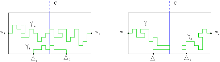
Figure 6. The two topologically distinct possibilities: either $\gamma_{1}$ connects $\Delta_{1}$ to $\Delta_{2}$, or it connects $w_{1}$ to $\Delta_{1}$. The fist case is very unlikely, see (A.18).

Let $C_{1}$ (resp. $C_{2}$) be the vertical column at distance $\lfloor L^{\varepsilon}\rfloor$ to the left (resp. to the right) of the column $C$. Then, one has the

Lemma A.4.

The probability that appears in Claim 3.10 can be upper bounded as

$$\pi_{\bar{A}}^{(-,+,\Delta)}(\Gamma^{c})\leq\pi_{V}^{\tau}(\bar{\Gamma}^{c}),$$ (A.16)

where

$$\bar{\Gamma}:=\{w_{i}\stackrel{{\scriptstyle\gamma_{i}}}{{\leftrightarrow}}\Delta_{i}\mbox{\; and\;}\gamma_{i}\cap C_{i}=\emptyset,i=1,2\}.$$ (A.17)

Therefore, from Theorem A.2 we see that to prove Claim 3.10 it is enough to show that

$$\frac{\mathcal{N}_{1}}{\Xi(V,\tau)}:=\frac{\sum_{\{\gamma_{1},\gamma_{2}\}\sim\tau}\Psi(\{\gamma_{1},\gamma_{2}\};V){\bf 1}_{\{\Delta_{1}\stackrel{{\scriptstyle\gamma_{1}}}{{\leftrightarrow}}\Delta_{2}\}}}{\Xi(V,\tau)}\leq e^{-cL^{3\varepsilon}}$$ (A.18)

and that

$$\frac{\mathcal{N}_{2}}{\Xi(V,\tau)}:=\frac{\sum_{\{\gamma_{1},\gamma_{2}\}\sim\tau}\Psi(\{\gamma_{1},\gamma_{2}\};V){\bf 1}_{\{\Delta_{1}\stackrel{{\scriptstyle\gamma_{1}}}{{\leftrightarrow}}w_{1}\}}{\bf 1}_{\{\gamma_{1}\cap C_{1}\neq\emptyset\}}}{\Xi(V,\tau)}\leq e^{-cL^{3\varepsilon}},$$ (A.19)

for some positive $c=c(\beta,\varepsilon)$.

Proof of Lemma A.4. Since the event $\Gamma^{c}$ is increasing, we note first of all that thanks to FKG we can enlarge the system from $\bar{A}$ to $V$ and change the b.c. from $(-,+,\Delta)$ to $\tau$. Secondly, we observe that the event $\bar{\Gamma}$ implies $\Gamma$. ∎

1.3.1. Lower bound on $\Xi(V,\tau)$

We will prove that there exists a positive constant $c^{\prime}$ such that for $\beta$ large

$$\Xi(V,\tau)\geq\exp\left(-\beta\tau_{\beta}(\vec{e}_{1})(L-c^{\prime}L^{3\varepsilon})\right).$$ (A.20)

Since we want a lower bound, we are allowed to keep only the configurations $\{\gamma_{1},\gamma_{2}\}\sim\tau$ such that $w_{i}\stackrel{{\scriptstyle\gamma_{i}}}{{\leftrightarrow}}\Delta_{i}$ and $\gamma_{i}$ does not touch the column $C_{i}$, for $i=1,2$. Call $\mathcal{G}_{i},i=1,2$ the set of configurations of $\gamma_{i}$ allowed by the above constraints.

Using the decay properties of $\Phi$, one sees that

$$\Xi(V,\tau)\geq c\,\left(\sum_{\gamma_{1}\in\mathcal{G}_{1}}\Psi(\gamma_{1};V)\right)^{2}.$$ (A.21)

The square is due to the fact that $\gamma_{1}$ and $\gamma_{2}$ essentially do not interact because their mutual distance is larger than $L^{\varepsilon}$ (the residual interaction can be bounded by a constant which is absorbed in $c$). It remains to prove that

$$\sum_{\gamma_{1}\in\mathcal{G}_{1}}\Psi(\gamma_{1};V)\geq\exp(-\beta\tau_{\beta}(\vec{e}_{1})((L/2)-c^{\prime}L^{3\varepsilon}))$$ (A.22)

for some positive $c^{\prime}$. This is an immediate consequence of Lemma A.6 below (applied with $\kappa=\varepsilon$), together with the fact that $d(w_{1},\Delta_{1})=L/2-L^{3\varepsilon}+O(L^{2\varepsilon})$, of the fact that the angle $\phi$ formed by the segment $w_{1}\Delta_{1}$ and $\vec{e}_{1}$ is $O(L^{-1/2+\varepsilon})$, and finally of the analyticity of the surface tension and its symmetry around $\vec{e}_{1}$.

1.3.2. Upper bound on $\mathcal{N}_{1}$

Using rough upper bounds on the number of paths $\gamma_{1}$ which connect $\Delta_{1}$ and $\Delta_{2}$ and the decay properties of $\Phi$ (in particular Lemma A.3), one sees that for $L$ large

$$\mathcal{N}_{1}\leq e^{-cL^{3\varepsilon}}\sum_{\gamma\subset\tilde{V}:\,w_{1}\stackrel{{\scriptstyle\gamma}}{{\leftrightarrow}}w_{2}}\Psi(\gamma;V)$$ (A.23)

for some $c=c(\beta,\varepsilon)>0$, where of course one uses the fact that $d(\Delta_{1},\Delta_{2})=2L^{3\varepsilon}$. Moreover, Theorem 4.16 of [9] ensures that

$$\sum_{{\gamma\subset\tilde{V}}:\,w_{1}\stackrel{{\scriptstyle\gamma}}{{\leftrightarrow}}w_{2}}\Psi(\gamma;V)\leq\exp(-\beta\tau_{\beta}(\vec{e}_{1})L+c(\log L)^{c}),$$ (A.24)

which, together with (A.20), concludes the proof of (A.18).

1.3.3. Proof of (A.19)

The estimate we wish to prove is very intuitive: if the path $\gamma_{1}$ makes a deviation to the right to touch the column $C_{1}$, it has an excess length, and therefore an excess energy, of order $L^{3\varepsilon}$ with respect to typical paths. The actual proof of (A.19) is a straightforward (although a bit lengthy) application of results from [9] and of the FKG inequalities. We sketch only the main steps.

First of all, letting $d(\gamma_{1},\gamma_{2}):=\min\{d(x_{1},x_{2}),x_{i}\in\gamma_{i},i=1,2\}$, we show that the contribution of the configurations such that $d(\gamma_{1},\gamma_{2})<L^{\varepsilon}$ is negligible. To this purpose, decompose first of all $\mathcal{N}_{2}$ as $\mathcal{N}_{2}=\mathcal{N}_{2}^{\prime}+\mathcal{N}_{2}^{\prime\prime}$ where

$$\mathcal{N}_{2}^{\prime}:=\sum_{\{\gamma_{1},\gamma_{2}\}\sim\tau}\Psi(\{\gamma_{1},\gamma_{2}\};V){\bf 1}_{\{\Delta_{1}\stackrel{{\scriptstyle\gamma_{1}}}{{\leftrightarrow}}w_{1}\}}{\bf 1}_{\{\gamma_{1}\cap C_{1}\neq\emptyset\}}{\bf 1}_{\{d(\gamma_{1},\gamma_{2})<L^{\varepsilon}\}}.$$ (A.25)

Consider the paths $\gamma_{i}$ as oriented from $w_{i}$ to $\Delta_{i}$ and, if $d(\gamma_{1},\gamma_{2})<L^{\varepsilon}$, call $P:=P(\gamma_{1},\gamma_{2}):=(x_{1},x_{2})\in{\mathbb{Z}^{2}}^{*}\times{\mathbb{Z}^{2}}^{*}$ where $x_{1}$ is the first point in $\gamma_{1}\cap{\mathbb{Z}^{2}}^{*}$ which is at distance less than $L^{\varepsilon}$ from $\gamma_{2}$, and $x_{2}$ is the first point in $\gamma_{2}\cap{\mathbb{Z}^{2}}^{*}$ at distance less than $L^{\varepsilon}$ from $x_{1}$. Of course, $P$ can take at most $L^{2}$ different values (this is a rough upper bound) and we can decompose $\mathcal{N}_{2}^{\prime}$ as $\mathcal{N}_{2}^{\prime}=\sum_{p}\mathcal{N}_{2,p}^{\prime}$ where $\mathcal{N}_{2,p}^{\prime}$ contains only the terms such that $P(\gamma_{1},\gamma_{2})=p$. Given $(\gamma_{1},\gamma_{2})$ such that $P(\gamma_{1},\gamma_{2})=p$, for $i=1,2$ one can write $\gamma_{i}$ as the union of $\gamma_{i}^{\prime}$ and $\gamma_{i}^{\prime\prime}$, where $\gamma_{i}^{\prime}$ connects $w_{i}$ to $x_{i}$, and $\gamma_{i}^{\prime\prime}$ connects $x_{i}$ to $\Delta_{i}$. Using the decay properties of $\Phi$ one sees that, uniformly in $p$ and in $\{\gamma_{i}^{\prime}\}_{i=1,2}$,

$$\sum_{\{\gamma_{i}^{\prime\prime}\}_{i=1,2}}\Psi(\{\gamma_{1},\gamma_{2}\};V)\leq c\Psi(\gamma_{1}^{\prime};V)\Psi(\gamma_{2}^{\prime};V),$$ (A.26)

where the sum runs over all the configurations of $\{\gamma_{i}^{\prime\prime}\}_{i=1,2}$ compatible with $\{\gamma_{i}^{\prime}\}_{i=1,2}$. Let $\Sigma$ be the set of paths $\gamma_{3}$ which connect $x_{1}$ to $x_{2}$, and such that the concatenation of $\gamma_{1}^{\prime},\gamma_{3}$ and $\gamma_{2}^{\prime}$ is an admissible open path, call it simply $\gamma$, connecting $w_{1}$ to $w_{2}$ and contained in $\tilde{V}$. Of course, the set $\Sigma$ depends on $\{\gamma_{i}^{\prime}\}_{i=1,2}$. Then, one sees that

$$\sum_{\{\gamma_{i}^{\prime\prime}\}_{i=1,2}}\Psi(\{\gamma_{1},\gamma_{2}\};V)\leq e^{cL^{\varepsilon}}\sum_{\gamma_{3}\in\Sigma}\Psi(\gamma;V).$$ (A.27)

In conclusion, summing over the admissible configurations of $\{\gamma_{i}^{\prime}\}_{i=1,2}$ and over the possible values of $p$, recalling (A.24) and the lower bound (A.20), we have shown that

$$\frac{\mathcal{N}_{2}^{\prime}}{\Xi(\tau,V)}\leq e^{-cL^{3\varepsilon}}.$$ (A.28)

As for $\mathcal{N}_{2}^{\prime\prime}$, using the decay properties of the potential $\Phi$ one sees immediately that, since $d(\gamma_{1},\gamma_{2})\geq L^{\varepsilon}$, the mutual interaction between the two paths can be bounded by a constant, so that

$${\mathcal{N}_{2}^{\prime\prime}}\leq c\;\sum_{\gamma_{1}\subset\tilde{V}:\;\;\Delta_{1}\stackrel{{\scriptstyle\gamma_{1}}}{{\leftrightarrow}}w_{1}}\Psi(\gamma_{1};V){\bf 1}_{\{\gamma_{1}\cap C_{1}\neq\emptyset\}}\times\sum_{\gamma_{2}\subset\tilde{V}:\;\;\Delta_{2}\stackrel{{\scriptstyle\gamma_{2}}}{{\leftrightarrow}}w_{2}}\Psi(\gamma_{2};V).$$ (A.29)

Recalling (A.21) one sees therefore that

$$\frac{\mathcal{N}_{2}^{\prime\prime}}{\Xi(\tau,V)}\leq c\frac{Q}{(1-Q)^{2}},$$ (A.30)

where

$$Q:=\frac{\sum_{\{\gamma\subset\tilde{V}:\;\;\Delta_{1}\stackrel{{\scriptstyle\gamma}}{{\leftrightarrow}}w_{1}\}}\Psi(\gamma;V){\bf 1}_{\{\gamma\cap C_{1}\neq\emptyset\}}}{\sum_{\{\gamma\subset\tilde{V}:\;\;\Delta_{1}\stackrel{{\scriptstyle\gamma}}{{\leftrightarrow}}w_{1}\}}\Psi(\gamma;V)}$$ (A.31)

and we are left with the task of proving that $Q\leq\exp(-cL^{3\varepsilon})$. Note that $Q$ is nothing but the equilibrium probability $\pi_{V}^{\hat{\tau}}(\gamma\cap C_{1}\neq\emptyset)$, where $\gamma$ is the unique open contour for a system enclosed in $V$ and with boundary conditions $\hat{\tau}$ given by $\hat{\tau}_{x}=+$ for $x=(i,0)$ with $i<\lfloor L/2\rfloor-L^{3\varepsilon}$ and $x=(0,i)$ with $i\leq 2\lfloor(2L+1)^{1/2+\varepsilon}\rfloor$, and $\hat{\tau}_{x}=-$ otherwise. Morally, one would like to apply [9, Th. 4.15] to say that $Q\leq\exp(-cL^{3\varepsilon})$; such result however cannot be applied directly because of the entropic repulsion effect that $\gamma$ feels due to the South border of $V$, and we need to take a small detour. Consider the $L$-shaped domain $W$ obtained as the union of the rectangles $V$ and $V^{\prime}$, where $V^{\prime}=\{(i,j)\in\mathbb{Z}^{2}:-L^{1/2+\varepsilon}\leq j\leq 0,1\leq i<\lfloor L/2\rfloor-L^{3\varepsilon}-1\}$, with boundary conditions $\hat{\tau}^{\prime}$ given by $\hat{\tau}^{\prime}=\hat{\tau}$ on $\partial W\cap\partial V$ and $\hat{\tau}^{\prime}=+$ on $\partial W\cap\partial V^{\prime}$, see Figure 7.

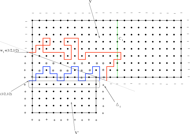
Figure 7. The $L$-shaped domain $W$ (for graphical convenience, proportions are not respected in the drawing) with its boundary conditions $\hat{\tau}^{\prime}$. For the construction of $\gamma^{\prime}$, one should imagine that the spins in the framed region are set to $-$. The sites marked by $*$ denote the $*$-connected set $\Delta^{+}(\gamma^{\prime})$. The drawn configuration of $\gamma$ is entirely above the straight line going through $w_{1}+(1/2,1/2)$ and $\Delta_{1}+(1/2,1/2)$, i.e. the spin configuration $\sigma$ belongs to the set $\Gamma^{\prime\prime}$ appearing in (A.36).

Below we will prove

Lemma A.5.

One has

$$Q=\pi_{V}^{\hat{\tau}}(\gamma\cap C_{1}\neq\emptyset)\leq\pi_{W}^{\hat{\tau}^{\prime}}(\gamma\cap C_{1}\neq\emptyset|\Gamma^{\prime})\leq\frac{\pi_{W}^{\hat{\tau}^{\prime}}(\gamma\cap C_{1}\neq\emptyset)}{\pi_{W}^{\hat{\tau}^{\prime}}(\Gamma^{\prime})},$$ (A.32)

where $\Gamma^{\prime}=\{\sigma\in\Omega_{W}:\;\exists$ inside $V$ a $*$-connected path of $+$ spins which connect the site $\Delta_{1}+(0,1)$ to one of the sites $(1,i)$ with $1\leq i\leq 2\lfloor(2L+1)^{1/2+\varepsilon}\rfloor\}$, see Figure 7.

The numerator in the right-hand side of (A.32) is smaller than $\exp(-cL^{3\varepsilon})$. Indeed, it suffices to remark that (cf. the notation (A.7)) it is smaller than

$$\frac{\mathcal{E}_{w_{1},\Delta_{1}}\left[{\bf 1}_{\{\gamma\cap C_{1}\neq\emptyset\}}\exp\left(\Phi_{W}(\gamma)\right)\right]}{\mathcal{E}_{w_{1},\Delta_{1}}\left[\exp\left(\Phi_{W}(\gamma)\right)\right]}\leq\frac{\sqrt{\mathcal{P}_{w_{1},\Delta_{1}}(\gamma\cap C_{1}\neq\emptyset)\mathcal{E}_{w_{1},\Delta_{1}}\left(\exp\left(2\Phi_{W}(\gamma)\right)\right)}}{\mathcal{E}_{w_{1},\Delta_{1}}\left[\exp\left(\Phi_{W}(\gamma)\right)\right]}.$$ (A.33)

where $\Phi_{W}(\gamma)$ was defined in (A.11). Theorem 4.15 of [9] says directly that

$$\mathcal{P}_{w_{1},\Delta_{1}}(\gamma\cap C_{1}\neq\emptyset)\leq\exp(-cL^{3\varepsilon}),$$

while the fast decay of $\Phi$, together with [9, Th. 4.16], implies that

$$\mathcal{E}_{w_{1},\Delta_{1}}\left[\exp\left(2\Phi_{W}(\gamma)\right)\right]\leq\exp(c(\log L)^{c})$$ (A.34)

$$\mathcal{E}_{w_{1},\Delta_{1}}\left[\exp\left(\Phi_{W}(\gamma)\right)\right]\geq\exp(-c(\log L)^{c}).$$ (A.35)

Roughly speaking, typical paths (under $\mathcal{P}_{w_{1},\Delta_{1}}$) have a small intersection with $W^{c}$ (again, the precise estimates follow from [9, Th. 4.15]). This is why we enlarged $V$ to $W$: if $W$ were replaced by $V$, the intersection would not be small any more and the expectations in (A.34)-(A.35) would not be under control.

The denominator in (A.32) is also not difficult to deal with: one observes (see Figure 7) that the event $\Gamma^{\prime}$ is implied by the event $\Gamma^{\prime\prime}=$$\{\gamma$ does not go below the straight line which goes through $\Delta_{1}+(1/2,1/2)$ and $w_{1}+(1/2,1/2)\}$ (we will write symbolically $\gamma\geq(\Delta_{1}w_{1})$). Indeed, the subset of $\Delta\gamma$ where spins are $+$ is $*$-connected and satisfies the requirements of $\Gamma^{\prime}$. Therefore, $\pi_{V}^{\hat{\tau}^{\prime}}(\Gamma^{\prime})\geq\exp(-cL^{\varepsilon})$. Indeed,

$$\pi_{V}^{\hat{\tau}^{\prime}}(\Gamma^{\prime})\geq\pi_{W}^{\hat{\tau}^{\prime}}(\Gamma^{\prime\prime})=\frac{\sum_{\gamma\sim\hat{\tau}^{\prime}}\Psi(\gamma;W){\bf 1}_{\{\gamma\geq(\Delta_{1}w_{1})\}}}{\sum_{\gamma\sim\hat{\tau}^{\prime}}\Psi(\gamma;W)}:$$ (A.36)

the numerator is lower bounded by

$$\exp[-\beta\tau_{\beta}(\vec{v}_{w_{1}\Delta_{1}})d(w_{1},\Delta_{1})-c(d(w_{1},\Delta_{1}))^{\varepsilon}]$$

via Lemma A.6 (take $\kappa=\varepsilon/2$) and the denominator is upper bounded by

$$\exp[-\beta\tau_{\beta}(\vec{v}_{w_{1}\Delta_{1}})d(w_{1},\Delta_{1})+c(\log d(w_{1},\Delta_{1}))^{c}]$$

via [9, Th. 4.16], where $\vec{v}_{w_{1}\Delta_{1}}$ is the unit vector pointing from $w_{1}$ to $\Delta_{1}$.

Summarizing, we have obtained $Q\leq\exp(-cL^{3\varepsilon})$ and, via (A.30) and (A.28), we have proven (A.19).

Proof of Lemma A.5. Given a configuration $\sigma\in\Omega_{W},$ imagine to replace all its spins in $\partial V\cap V^{\prime}$ by $-$, cf. Figure 7; then, associated to the restriction $\sigma_{V}\in\Omega_{V}$, there are exactly two open contours in $\tilde{V}$. The endpoints of these two contours are $(1/2,1/2)$, $w_{1}+(1/2,1/2)$, $\Delta_{1}+(1/2,1,2)$ and $\Delta_{1}+(-1/2,1/2)$. Under the assumption that $\sigma\in\Gamma^{\prime}$, one sees immediately that one of the two contours connects $w_{1}$ to $\Delta_{1}$ (this is nothing else but the open contour which we have called $\gamma$ so far, e.g. in (A.32)); we will call $\gamma^{\prime}$ the second open contour, see Figure 7. Given a possible configuration for $\gamma^{\prime}$, $V$ is divided into two components, call them $V^{\pm}(\gamma^{\prime})$, where $V^{-}(\gamma^{\prime})$ is the one “in contact with” $V^{\prime}$. It is clear that the intersection $\Delta^{+}(\gamma^{\prime}):=\Delta\gamma^{\prime}\cap V^{+}(\gamma^{\prime})$ is a $*$-connected set (i.e. any two of its points can be linked by a $*$-connected chain belonging to $\Delta^{+}(\gamma^{\prime})$) and all spins are $+$ there. It is important to remark that if we take $\sigma\in\Gamma^{\prime}$ and flip any spin in $V_{\gamma^{\prime}}^{int}:=V^{+}(\gamma^{\prime})\setminus\Delta^{+}(\gamma^{\prime})$, the configuration of $\gamma^{\prime}$ does not change. Also, if (with abuse of notation) we let $\pi_{\gamma^{\prime}}$ denote the equilibrium measure in $V_{\gamma^{\prime}}^{int}$ with b.c. $+$ on the portion of the boundary which coincides with $\Delta^{+}(\gamma^{\prime})$ and $\hat{\tau}$ otherwise, one has

$$\pi_{\gamma^{\prime}}(\gamma\cap C_{1}\neq\emptyset)\geq\pi_{V}^{\hat{\tau}}(\gamma\cap C_{1}\neq\emptyset),$$ (A.37)

by FKG since the event $\gamma\cap C_{1}\neq\emptyset$ is increasing. One has then, with $\mathcal{S}$ the set of possible configurations of $\gamma^{\prime}$,

$$\frac{\pi_{W}^{\hat{\tau}^{\prime}}(\gamma\cap C_{1}\neq\emptyset)}{\pi_{W}^{\hat{\tau}^{\prime}}(\Gamma^{\prime})} \geq \frac{\pi_{W}^{\hat{\tau}^{\prime}}(\gamma\cap C_{1}\neq\emptyset;\Gamma^{\prime})}{\pi_{W}^{\hat{\tau}^{\prime}}(\Gamma^{\prime})}$$

$$= \sum_{\xi\in\mathcal{S}}{\pi_{W}^{\hat{\tau}^{\prime}}(\gamma\cap C_{1}\neq\emptyset|\Gamma^{\prime};\gamma^{\prime}=\xi)}\frac{\pi_{W}^{\hat{\tau}^{\prime}}(\Gamma^{\prime};\gamma^{\prime}=\xi)}{\pi_{W}^{\hat{\tau}^{\prime}}(\Gamma^{\prime})}$$

$$= \sum_{\xi\in\mathcal{S}}\pi_{\xi}(\gamma\cap C_{1}\neq\emptyset)\frac{\pi_{W}^{\hat{\tau}^{\prime}}(\Gamma^{\prime};\gamma^{\prime}=\xi)}{\pi_{W}^{\hat{\tau}^{\prime}}(\Gamma^{\prime})}\geq\pi_{V}^{\hat{\tau}}(\gamma\cap C_{1}\neq\emptyset),$$

where we used (A.37) in the second inequality. ∎

1.3.4. A technical lemma

Let $a:=(a_{1},a_{2})\in{\mathbb{Z}^{2}}^{*}$ and $b=(b_{1},b_{2})\in{\mathbb{Z}^{2}}^{*}$ with $b_{1}>a_{1}$. Let $\vec{v}_{ab}$ be the unit vector pointing from $a$ to $b$ and $\phi_{ab}$ be the angle which $\vec{v}_{ab}$ forms with $\vec{e}_{1}$. Assume that $-\pi/4\leq\phi_{ab}\leq\pi/4$. Let $A>0,\kappa>0$, let $U_{a,b}=U_{a,b}(A,\kappa)\subset{\mathbb{R}}^{2}$ be the cigar-shaped region which is delimited by the two curves

$$x\mapsto\xi^{\pm}_{a,b;A,\kappa}(x):=x\tan(\phi_{ab})\pm A\left(\frac{(x-a_{1})(b_{1}-x)}{b_{1}-a_{1}}\right)^{1/2+\kappa},\;\;x\in[a_{1},b_{1}],$$

and $U^{+}_{a,b}$ be the upper half of $U_{a,b}$, obtained by slicing $U_{a,b}$ along the segment $ab$. Also, we will denote by $\Sigma_{a,b}=\Sigma_{a,b}(A,\kappa)$ the set of all open contours $\gamma$ having $a$ and $b$ as endpoints, and such that every bond in $\gamma$ has non-empty intersection with $U_{a,b}$; similarly we define $\Sigma^{+}_{a,b}$. Then,

Lemma A.6.

Let $\beta$ be large enough, and consider a domain $V\subset\mathbb{Z}^{2}$ such that $\tilde{V}$ contains $U^{+}_{a,b}(A,\kappa)$ (cf. Definition A.1). There exists $c$ depending on $\beta,A,\kappa$ such that

$$\sum_{\gamma\in\Sigma^{+}_{a,b}}\Psi(\gamma;V)\geq\exp\left[-\beta\tau_{\beta}(\vec{v}_{ab})d(a,b)-c(d(a,b))^{2\kappa}\right].$$ (A.39)

This result can be obtained via a repeated use of Theorem 4.16 of [9]. The error term $\exp(-c\,(d(a,b))^{2\kappa})$ is very rough (but sufficient for our purposes) and can presumably be improved. We do not give full details because they are a bit lengthy, although standard, but we sketch the main steps.

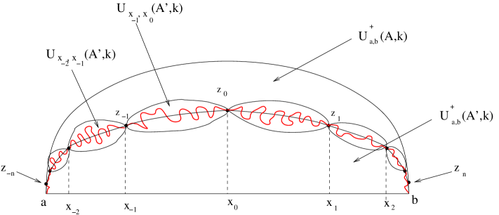
Figure 8. A typical path $\gamma$ which contributes to the lower bound (A.39). For graphical convenience, we have assumed that $a$ and $b$ have the same vertical coordinate, and not all the cigar-shaped sets $U_{z_{i},z_{i+1}}(A^{\prime},\kappa)$ have been drawn.

First of all, let for simplicity of notations $L:=b_{1}-a_{1}$ and $A^{\prime}:=A/10$. Then, one proceeds as follows (keep in mind Figure 8):

• for every $-n\leq i\leq n$, with $n=\log_{2}(L)-2$, let $z_{i}=(x_{i},y_{i})$ be a point in ${\mathbb{Z}^{2}}^{*}$ at minimal distance from $(\tilde{x}_{i},\xi^{+}_{a,b;A^{\prime},\kappa}(\tilde{x}_{i}))$, where

  $$\tilde{x}_{i}:=a_{1}+(b_{1}-a_{1})\left(\frac{1}{2}+\frac{{\rm sign}(i)}{4}\sum_{j=0}^{|i|-1}2^{-j}\right);$$ (A.40)

• remark via elementary geometrical considerations that for every $-n\leq i<n$, the cigar-shaped set $U_{z_{i},z_{i+1}}(A^{\prime},\kappa)$ is entirely contained in $U^{+}_{a,b}(A,\kappa)$;

• restrict the sum (A.39) to the paths $\gamma$ which, when oriented from $a$ to $b$, go through the points $z_{-n},z_{-n+1},\ldots,z_{n}$ (in this order), and such that the portion of the path between $z_{i}$ and $z_{i+1}$ belongs to $\Sigma_{z_{i},z_{i+1}}(A^{\prime},\kappa)$;

• remark that, via the decay properties of the potential $\Phi$, the interaction between two adjacent portions of $\gamma$ just defined can be bounded above by a constant;

• apply Theorem 4.16 of [9] to write that for every $-n\leq i<n$ one has

  $$\sum_{\gamma\in\Sigma_{z_{i},z_{i+1}}(A^{\prime},\kappa)}\Psi(\gamma;V)\geq\exp\left[-\beta\tau_{\beta}(\vec{v}_{z_{i},z_{i+1}})d(z_{i},z_{i+1})-c(\log d(z_{i},z_{i+1}))^{c}\right],$$ (A.41)

  for some constant $c$ depending on $A,\kappa,\beta$. As for the two portions of $\gamma$ from $a$ to $z_{-n}$ and from $z_{n}$ to $b$, they give a multiplicative contribution of order $1$ to (A.39) (this is because $d(a,z_{-n})=O(1)$ and $d(b,z_{n})=O(1)$, as is immediately seen from the definition of $n$);

• put together the estimates on the contributions coming from the $2n+3$ portions of $\gamma$ obtained in the previous point: using the convexity and smoothness properties of the surface tension $\tau_{\beta}(\cdot)$, one obtains the claim of the lemma.

References

- [1] K. S. Alexander, The Spectral Gap of the 2-D Stochastic Ising Model with Nearly Single-Spin Boundary Conditions, J. Statist. Phys. 104 (2001), 59–87.
- [2] K. S. Alexander, N. Yoshida, The spectral gap of the 2-D stochastic Ising model with mixed boundary conditions, J. Statist. Phys. 104 (2001), 89–109.
- [3] Y. Higuchi, N. Yoshida, Slow relaxation of -D stochastic Ising models with random and non-random boundary conditions, New trends in stochastic analysis, Charingworth, (1994), 153–167.
- [4] R. H. Schonmann, N. Yoshida, Exponential relaxation of Glauber dynamics with some special boundary conditions, Comm. Math. Phys. 189 (2) (1997), 299–309.
- [5] A. Bianchi, Glauber dynamics on non-amenable graphs: boundary conditions and mixing time, Electron. J. Probab. 13 (2008), 1980–2012.
- [6] T. Bodineau and F. Martinelli, Some new results on the kinetic Ising model in a pure phase, J. Statist. Phys. 109 (2002), 207–235.
- [7] P. Caputo, F. Martinelli, and F. L. Toninelli, On the approach to equilibrium for a polymer with adsorption and repulsion, Electron. J. Probab. 13, 213–258 (2008).
- [8] F. Cesi, G. Guadagni, F. Martinelli, and R. H. Schonmann, On the 2D stochastic Ising model in the phase coexistence region close to the critical point, J. Statist. Phys. 85 (1996), 55–102.
- [9] R. Dobrushin, R. Kotecký, S. Shlosman, Wulff Construction. A global Shape from Local Interaction, Transl. Math. Monographs 104, American Mathematical Society, Providence, RI, 1992.
- [10] D. S. Fisher, D. A. Huse, Dynamics of droplet fluctuations in pure and random Ising systems, Phys. Rev. B 35 (1987), 6841–6846.
- [11] C. M. Fortuin, P. W. Kasteleyn, J. Ginibre, Correlation inequalities on some partially ordered sets, Comm. Math. Phys. 22 (1971), 89–103.
- [12] Y. Higuchi and J. Wang, Spectral gap of Ising model for Dobrushin’s boundary condition in two dimensions, preprint, 1999.
- [13] T. M. Liggett, Interacting particle systems, Springer Verlag, New York, 1985.
- [14] D. A. Levin, Y. Peres, E. L. Wilmer, Markov Chains and Mixing Times, American Mathematical Society, Providence, RI, 2009.
- [15] D. Levin, M. Luczak, Y. Peres, Glauber dynamics for the Mean-field Ising Model: cut-off, critical power law, and metastability, Probab. Theory Related Fields, in press, (2009)
- [16] F. Martinelli, On the two dimensional dynamical Ising model in the phase coexistence region, J. Statist. Phys. 76 (1994), 1179–1246.
- [17] F. Martinelli, Lectures on Glauber dynamics for discrete spin models, Lecture Notes in Math. 1717, Springer, Berlin, (1999).
- [18] F. Martinelli, A. Sinclair, and D. Weitz, Glauber dynamics on trees: Boundary conditions and mixing time, Comm. Math. Phys. 250 (2) (2004), 301–334.
- [19] F. Martinelli, A. Sinclair, Mixing time for the solid-on-solid model, Proceedings of the 41st Annual ACM Symposium on Theory of Computing (STOC), pp. 571–580 (2009).
- [20] A. Martin-Löf, Mixing properties, differentiability of the free energy and the central limit theorem for a pure phase in the Ising model at low temperature, Comm. Math. Phys. 32 (1973), 75–92.
- [21] A. Messager, S. Miracle-Solé, and J. Ruiz, Convexity properties of the surface tension and equilibrium crystals, J. Statist. Phys. 67 (1992), 449–470.
- [22] Y. Peres, Mixing for Markov Chains and Spin Systems, available at www.stat.berkeley.edu/~peres/ubc.pdf
- [23] S. Shlosman, The droplet in the tube: a case of phase transition in the canonical ensemble, Comm. Math. Phys. 125 (1989), 81–90.
- [24] B. Simon, The statistical mechanics of lattice gases. Vol. I. Princeton Series in Physics. Princeton University Press, Princeton, NJ, 1993.
- [25] N. Sugimine, A lower bound on the spectral gap of the 3-dimensional stochastic Ising models, J. Math. Kyoto Univ. 42 (2002), 751–788.
- [26] N. Sugimine, Extension of Thomas’ result and upper bound on the spectral gap of -dimensional stochastic Ising models, J. Math. Kyoto. Univ. 42 (1) (2002), 141–160.
- [27] L. E. Thomas, Bound on the mass gap for finite volume stochastic Ising models at low temperature, Comm. Math. Phys. 126 (1989), 1–11.