Numerical evaluation of convex-roof entanglement measures
with applications to spin rings

Abstract

We present two ready-to-use numerical algorithms to evaluate convex-roof extensions of arbitrary pure-state entanglement monotones. Their implementation leaves the user merely with the task of calculating derivatives of the respective pure-state measure. We provide numerical tests of the algorithms and demonstrate their good convergence properties. We further employ them in order to investigate the entanglement in particular few-spins systems at finite temperature. Namely, we consider ferromagnetic Heisenberg exchange-coupled spin-$\frac{1}{2}$ rings subject to an inhomogeneous in-plane field geometry obeying full rotational symmetry around the axis perpendicular to the ring through its center. We demonstrate that highly entangled states can be obtained in these systems at sufficiently low temperatures and by tuning the strength of a magnetic field configuration to an optimal value which is identified numerically.

I Introduction

Entanglement, one of the most intriguing features of quantum mechanics Schrödinger (1935); Einstein et al. (1935), is undoubtedly an indispensable ingredient as a resource to any quantum computation or quantum communication scheme Nielsen and Chuang (2000). The ability to (sometimes drastically) outperform classical computations using multipartite quantum correlations has been demonstrated in various theoretical proposals which by now have become well known standard examples Deutsch and Jozsa (1992); Cleve et al. (1998); Grover (1996); Shor (1997). Due to the rapid progress in the fields of quantum computation, communication, and cryptography, both on the theoretical and the experimental side, it has become a necessity to quantify and study the production, manipulation and evolution of entangled states theoretically.

However, this has turned out to be a rather difficult task, as the dimension of the state space of a quantum system grows exponentially with the number of qudits and thus permits the existence of highly nontrivial quantum correlations between parties. While bipartite entanglement is rather well understood (see, e.g., Plenio and Virmani (2007)), the study of multipartite states (with three or more qudits) is an active field of research.

Several different approaches towards the study of entanglement exist. Bell’s original idea Bell (1964) that certain quantum states can exceed classically strict upper bounds on expressions of correlators between measurement outcomes of different parties sharing the same state has been widely extended and improved to detect entanglement in a great variety of states. Entanglement between photons persisting over large distances has been demonstrated with the use of Bell-type inequalities (see, e.g., Ref. Ursin et al. (2007) and references therein). Another more recent approach is the concept of entanglement witnesses Horodecki et al. (1996); Terhal (2000). These are observables whose expectation value is non-negative for separable states and negative for some entangled states. Thirdly, the concept of entanglement measures is focussing more on the quantification of entanglement: if state $A$ has lower entanglement than state $B$, then $A$ cannot be converted into $B$ by means of local operations and classical communication. Remarkably, there exist interesting relations between entanglement measures and Bell inequalities Emary and Beenakker (2004) on the one hand, and entanglement witnesses Gühne et al. (2007); Eisert et al. (2007) on the other hand. In this work, we focus on the direct evaluation of entanglement measures.

Among the many features one can demand of such a measure, monotonicity is arguably the most important one: an entanglement measure should be non-increasing under local operations and classical communication (reflecting the fact that it is impossible to create entanglement in a separable state by these means). A measure exhibiting this property is called an entanglement monotone, with prominent examples being, e.g., the entanglement of formation Bennett et al. (1996a), the tangle Coffman et al. (2000), the concurrence Mintert et al. (2005a) or the measure by Meyer and Wallach Meyer and Wallach (2002). While one measure captures certain features of some states especially well, other measures focus on different aspects of different states.

Often, entanglement monotones are defined only for pure states and are given as analytical expressions of the state’s components in a standard basis. Unfortunately, quantifying mixed-state entanglement is more involved. This is somewhat intuitive, since the measure needs to be capable of distinguishing quantum from classical correlations. A manifestation of this difficulty is the fact that the problem of determining whether a given density matrix is separable or not is apparently very hard and has no known general solution for an arbitrary number of subsystems with arbitrary dimensions. The ability to study mixed-state entanglement is, however, highly desirable since mixed-states appear naturally due to various coupling mechanisms of the system under examination to its environment. There exists a standard way to construct a mixed-state entanglement monotone from a pure-state monotone, the so-called convex-roof construction Uhlmann (2000), but the evaluation of functions obtained in this way requires the solution of a rather involved constrained optimization problem (see Sec. II).

In this paper, we present two algorithms targeted at solving this optimization problem numerically for any given convex-roof entanglement measure. In principle, these algorithms can also be applied to any optimization problem subjected to the same kind of constraints. The first algorithm is an extension of a procedure originally used to calculate the entanglement of formation Audenaert et al. (2001). It is a conjugate gradient method exploiting the geometric structure of the nonlinear search space emerging from the optimization constraint. The second algorithm is based on a real parametrization of the search space, which allows one to carry out the optimization problem in the more familiar Euclidean space using standard techniques.

In the second part of the paper, we use these algorithms in order to study the entanglement properties of a certain type of spin rings. These systems form a generalization to $N$ qubits of our previous study, where we had only considered the case $N=3$ Röthlisberger et al. (2008). In the presence of an isotropic and ferromagnetic Heisenberg interaction and local in-plane magnetic fields obeying a radial symmetry, it can be argued (see Sec. IV and Ref. Röthlisberger et al. (2008)) that the ground state becomes a local unitary equivalent of an almost perfect N-partite Greenberger-Horne-Zeilinger (GHZ) state Greenberger et al. (1989)

$$|\mathrm{GHZ}_{N}^{\pm}\rangle=\left(|{\uparrow\uparrow\ldots\uparrow}\rangle\pm|{\downarrow\downarrow\ldots\downarrow}\rangle\right)/\sqrt{2}.$$ (1)

Such a system could hence be used for the production of highly entangled multipartite states merely by cooling it down to low temperatures. One finds, however, that the energy splitting between the ground and first excited state vanishes in the same limit as the N-partite approximate GHZ states become perfect, namely for the magnetic field strength going to zero. Therefore, in order to quantitatively identify the magnetic field strengths yielding maximal entanglement at finite temperature, one has to study the system in terms of a suitable mixed-state entanglement measure.

The outline of the paper is as follows: In Sec. II we review how the evaluation of a convex-roof entanglement measure is related to a constrained optimization problem. We then develop and describe the numerical algorithms capable of tackling this problem in Sec. III. We also present some benchmark tests, comparing our methods to another known algorithm. In Sec. IV, we describe the spin rings mentioned earlier and study their entanglement properties in terms of a convex-roof entanglement measure evaluated using our algorithms. We conclude our work in Sec. V.

II Convex-roof entanglement measures as constrained optimization problems

Given a pure-state entanglement monotone $m$, the most reasonable properties one can demand of a generalization of $m$ to mixed states are that this generalization is itself an entanglement monotone, and that it properly reduces to $m$ for pure states. A standard procedure which achieves this is the so-called convex-roof construction Uhlmann (2000); Mintert et al. (2005b). Given a mixed state $\rho$ acting on a Hilbert space $\mathcal{H}$ of finite dimension $d$, it is defined as

$$M(\rho)=\inf_{\{p_{i},|\psi_{i}\rangle\}\in\mathfrak{D}(\rho)}\sum_{i}p_{i}m(|\psi_{i}\rangle),$$ (2)

where

$$\mathfrak{D}(\rho)=\Bigl{\{}\left\{p_{i},|\psi_{i}\rangle\right\}_{i=1}^{s},s\geq\mathop{\mathrm{missing}}{rank}\rho\;\big{|}\;\{|\psi_{i}\rangle\}_{i=1}^{s}\subset\mathcal{H},\\ p_{i}\geq 0,\;\sum_{i=1}^{s}p_{i}=1,\;\rho=\sum_{i=1}^{s}p_{i}|\psi_{i}\rangle\langle\psi_{i}|\Bigr{\}}$$ (3)

is the set of all pure-state decompositions of $\rho$. Note that the pure states $|\psi_{i}\rangle$ are understood to be normalized. The numerical value of $M(\rho)$ is hence defined as an optimization problem over the set $\mathfrak{D}(\rho)$.

In order to apply numerical algorithms to this problem, $\mathfrak{D}(\rho)$ must be accessible in a parametric way. This parametrization is well-known and is often referred to as the Schrödinger-HJW theorem Hughston et al. (1993); Kirkpatrick (2005), which we briefly outline here for the sake of completeness.

Let $St(k,r)$ denote the set of all $k\times r$ matrices $U\in\mathds{C}^{k\times r}$ with the property $U^{\dagger}U=1_{r\times r}$, i.e., matrices with orthonormal column vectors (hence we have $k\geq r$). The first part of the Schrödinger-HJW theorem states that every $U\in St(k,r)$ yields a pure-state decomposition $\{p_{i},|\psi_{i}\rangle\}_{i=1}^{k}\in\mathfrak{D}(\rho)$ of the density matrix $\rho$ by the following construction. Let $\lambda_{i}$, $|\chi_{i}\rangle$, $i=1,\ldots,r=\mathop{\mathrm{missing}}{rank}\rho$ denote the eigenvalues and corresponding normalized eigenvectors of $\rho$, i.e.,

$$\rho=\sum_{i=1}^{r}\lambda_{i}|\chi_{i}\rangle\langle\chi_{i}|.$$ (4)

Note that we have $\lambda_{i}>0$ since $\rho$ is a density matrix and as such a positive semi-definite operator. Given a matrix $U\in St(k,r)$, define the auxiliary states

$$|\tilde{\psi}_{i}\rangle=\sum_{j=1}^{r}U_{ij}\sqrt{\lambda_{j}}|\chi_{j}\rangle,\qquad i=1,\ldots,k.$$ (5)

It is then readily checked that

$$p_{i}=\langle\tilde{\psi}_{i}|\tilde{\psi}_{i}\rangle,$$ (6)

$$|\psi_{i}\rangle=(1/\sqrt{p_{i}})|\tilde{\psi}_{i}\rangle$$ (7)

is indeed a valid decomposition of $\rho$ into a convex sum of $k$ projectors.

The second part of the theorem states that for any given pure-state decomposition $\{p_{i},|\psi_{i}\rangle\}_{i=1}^{k}$ of $\rho$, there exists a $U\in St(k,r)$ realizing the decomposition by the above construction. This guarantees that by searching over the set $St(k,r)$ and obtaining the decompositions according to the Schrödinger-HJW theorem, we do not ‘miss out’ on any part of the subset of $\mathfrak{D}(\rho)$ with a fixed number of states $k$. The parameterization is thus complete, i.e., searching the infimum over $St(k,r)$ is equivalent to searching over all decompositions with fixed so-called cardinality $k$. This allows us to reformulate the optimization problem Eq. (2) as

$$M(\rho)=\min_{k\geq r}\inf_{U\in St(k,r)}h(U),$$ (8)

where $h(U)$ is the sum on the right-hand side of Eq. (2) obtained via the matrix $U$ from $\rho$, i.e.,

$$h(U)=\sum_{i=1}^{k}p_{i}(U)m(|\psi_{i}(U)\rangle).$$ (9)

Note that we have dropped the $\rho$-dependence in the above expressions, since $\rho$ is fixed within a particular calculation and only the dependence of $h$ on $U$ is of relevance in the following.

It is clear that in a numerical calculation only a finite number of different values for $k$ can be investigated. However, it is also intuitive to expect that for some large enough value of $k$, increasing the latter even further has only marginal effects. In fact, we have observed numerically that already $k=\mathop{\mathrm{missing}}{rank}\rho+4$ yields very accurate results in all tests we have performed (also in the ones presented in Sec. III.3), and we have used this choice throughout all numerical calculations within this work. Note that for a fixed value of $k$, also all other decompositions with cardinality smaller than $k$ are considered as well, since the probabilities $p_{i}$ in the elements of $\mathfrak{D}(\rho)$ are allowed to go to zero (with the convention that the corresponding states $|\psi_{i}\rangle$ are then discarded).

Since the algorithms presented in the next section will both be gradient-based, the derivatives of Eq. (9) with respect to the real and imaginary parts of $U$ evaluated at $U$ will be required at some point. We state them here for the convenience of the reader. They are given by

$$\frac{\partial h}{\partial\mathop{\mathrm{missing}}{Re}U_{kl}} =2\lambda_{l}\mathop{\mathrm{missing}}{Re}(U_{kl})m(|\psi_{k}(U)\rangle)+\sum_{i=1}^{d}\left[\mathop{\mathrm{missing}}{Re}\phi^{(i)}_{R,kl}\left.\frac{\partial m}{\partial\mathop{\mathrm{missing}}{Re}\psi^{(i)}}\right|_{|\psi_{k}(U)\rangle}+\mathop{\mathrm{missing}}{Im}\phi^{(i)}_{R,kl}\left.\frac{\partial m}{\partial\mathop{\mathrm{missing}}{Im}\psi^{(i)}}\right|_{|\psi_{k}(U)\rangle}\right],$$ (10)

$$\frac{\partial h}{\partial\mathop{\mathrm{missing}}{Im}U_{kl}} =2\lambda_{l}\mathop{\mathrm{missing}}{Im}(U_{kl})m(|\psi_{k}(U)\rangle)+\sum_{i=1}^{d}\left[\mathop{\mathrm{missing}}{Re}\phi^{(i)}_{I,kl}\left.\frac{\partial m}{\partial\mathop{\mathrm{missing}}{Re}\psi^{(i)}}\right|_{|\psi_{k}(U)\rangle}+\mathop{\mathrm{missing}}{Im}\phi^{(i)}_{I,kl}\left.\frac{\partial m}{\partial\mathop{\mathrm{missing}}{Im}\psi^{(i)}}\right|_{|\psi_{k}(U)\rangle}\right],$$ (11)

where

$$|\phi_{R,kl}(U)\rangle =\left[\sqrt{p_{k}(U)\lambda_{l}}|\chi_{l}\rangle-\lambda_{l}\mathop{\mathrm{missing}}{Re}(U_{kl})|\psi_{k}(U)\rangle\right],$$ (12)

$$|\phi_{I,kl}(U)\rangle =\left[\mathfrak{i}\sqrt{p_{k}(U)\lambda_{l}}|\chi_{l}\rangle-\lambda_{l}\mathop{\mathrm{missing}}{Im}(U_{kl})|\psi_{k}(U)\rangle\right],$$ (13)

and superscripts such as in $\psi^{(i)}$ denote the $i$th component of the state $|\psi\rangle$ in an arbitrary but fixed basis.

As a last remark, we would like to point out that the constraint set $St(k,r)$ is, in fact, a closed embedded submanifold of $\mathds{C}^{k\times r}$, called the complex Stiefel manifold Absil et al. (2008). The geometric structure emerging thereof is exploited in one of the two algorithms following shortly. The dimension of the Stiefel mainfold is $\dim St(k,r)=2kr-r^{2}$ Absil et al. (2008). Since we have $k\geq r$, we can set $k=r+n$, $n=0,1,\ldots$. The number of free parameters $N$ in the optimization is thus $N=r^{2}+2nr$. Hence, $N$ grows linearly with $n$, but quadratically with $r$. Numerical evaluation in larger systems will thus be restricted to low-rank density matrices. The flexibility of choosing $n$ is however less restricted. As mentioned above, $n=4$ already yields satisfying results.

III Numerical Algorithms

The study of optimization problems on matrix manifolds is a rather new and still active field of research (see Edelman et al. (1998); Absil et al. (2008) and references therein). Only recently, two ready-to-use algorithms for minimization over the complex Stiefel manifold have been presented Manton (2002). To our knowledge, these are the only general purpose algorithms applicable to generic target functions over $St(k,r)$ found in the literature. One is a steepest descent-type method, the other one is of Newton-type. We will compare the performance of the modified steepest descent algorithm, as it is referred to in the original work, with the methods presented in this section. We have found that our algorithms generally show better convergence properties in the cases we have examined.

We will, however, not make use of the modified Newton algorithm for the following reasons. The second derivatives (as required by any Newton-type algorithm) of the function $h(U)$ [Eq. (9)] are in general quite involved and their number grows quadratically with the size of $U$. Hence, they are very expensive to evaluate, even if one resorts to numerical finite differences. Moreover, the good convergence properties of Newton-type methods may only be expected in the very proximity of a local minimum. One therefore first typically employs gradient-based techniques to approach a minimum sufficiently enough. However, what ‘sufficiently enough’ means in a particular case is often not known beforehand. We will later make use of a quasi-Newton algorithm, which approaches local minima satisfyingly and shows strong convergence similar to Newton methods automatically when being close enough to a minimum.

III.1 Generalized Conjugate-Gradient Method

In Ref. Audenaert et al. (2001) a conjugate-gradient algorithm on the unitary group $U(k)=St(k,k)$ was presented. The goal there was to calculate the entanglement of formation also for systems with dimensions different from $2\times 2$ Wootters (1998). Here, we extend this result by noting that the method is applicable to any optimization problem on $St(k,k)$, particularly to the evaluation of entanglement measures other than the entanglement of formation, and we calculate the required general expression of the gradient of $h(U)$.

Optimizing over $St(k,k)$ instead of $St(k,r)$ comes at the cost of over-parameterizing the search space. When using this algorithm to calculate convex-roof entanglement measures, we simply took into account only the first $r$ columns of the matrix obtained at every iteration. This is certainly an aspect one could improve upon in future research.

The algorithm presented here is a conjugate gradient-type method, meaning that instead of simply going downhill, i.e., in the direction of steepest descent, previous search directions are taken into account at the current iteration step. Once the search direction $X_{i}$ at iteration step $i$, a skew-Hermitian $k\times k$ matrix, is known, a line search along the geodesic $U_{i}\exp({tX_{i}})$ is performed, where $U_{i}$ is the current iteration point. In particular, one iteration step of the algorithm may be described as follows Audenaert et al. (2001):

1. Perform a line minimization, i.e., set

   $${t_{i+1}\leftarrow\arg\min_{t}h(U_{i}\exp{(tX_{i})})}$$ (14)

   and set

   $$U_{i+1}\leftarrow U_{i}\exp{(t_{i+1}X_{i})}.$$ (15)

2. Compute the new gradient $G_{i+1}$ at $U_{i+1}$ and set

   $$T\leftarrow\exp(t_{i+1}X_{i}/2)G_{i}\exp(-t_{i+1}X_{i}/2).$$ (16)

   $T$ is the gradient $G_{i}$ parallel-transported to the new point $U_{i+1}$.

3. Calculate the modified Polak-Ribière parameter

   $$\gamma\leftarrow\frac{\langle G_{i+1}-T,G_{i+1}\rangle}{\langle G_{i},G_{i}\rangle},$$ (17)

   where $\langle X,Y\rangle=\mathop{\mathrm{missing}}{Tr}\nolimits XY^{\dagger}$.

4. Set the new search direction to

   $$X_{i+1}\leftarrow-G_{i+1}+\gamma X_{i}.$$ (18)

5. $i\leftarrow i+1$.

6. Repeat from step 1 until convergence.

The starting point $U_{0}$ can be chosen arbitrarily, and the initial search direction is set to $X_{0}=-G_{0}$. In order to find a good approximation to the global minimum, one should restart the procedure several times using random initial conditions. For the line search in step 1, we utilized the derivative-free algorithm linmin described in Ref. Press et al. (1992).

In the following, we calculate the general expression for the gradient $G$ of the function $h$, evaluated at the point $U$ (we drop iteration indices for simplicity). The gradient $G$ is defined in terms of the directional derivative of $h$, namely as

$${\frac{dh(U^{(\varepsilon)}(X))}{d\varepsilon}}\bigg{|}_{\varepsilon=0}=\langle G,X\rangle,$$ (19)

where $U^{(\varepsilon)}(X)=V\exp(\varepsilon X)$ is a geodesic on $St(k,k)$ in direction $X$ (skew-Hermitian matrix) and passing through $V$. The inner product is defined as in step 3 of the algorithm. We will eventually read off the gradient $G$ from its definition in Eq. (19).

Treating $h(U)$ as a function of the real and imaginary matrix elements of $U$, $\mathop{\mathrm{missing}}{Re}U_{ik}$ and $\mathop{\mathrm{missing}}{Im}U_{ik}$, respectively, we have

$$\begin{split}{\frac{dh(U^{(\varepsilon)}(X))}{d\varepsilon}}\bigg{|}_{\varepsilon=0}&=\sum_{ik}\left(\frac{\partial h}{\partial\mathop{\mathrm{missing}}{Re}U_{ik}}\bigg{|}_{V}\frac{\partial\mathop{\mathrm{missing}}{Re}U^{(\varepsilon)}_{ik}}{\partial\varepsilon}\bigg{|}_{\epsilon=0}\right.\\ &\quad\left.+\frac{\partial h}{\partial\mathop{\mathrm{missing}}{Im}U_{ik}}\bigg{|}_{V}\frac{\partial\mathop{\mathrm{missing}}{Im}U^{(\varepsilon)}_{ik}}{\partial\varepsilon}\bigg{|}_{\epsilon=0}\right).\end{split}$$ (20)

The partial derivatives of $h$ with respect to $\mathop{\mathrm{missing}}{Re}U_{ik}$ and $\mathop{\mathrm{missing}}{Im}U_{ik}$ have already been stated in Eqs. (10, 11). Inserting the derivatives of $U_{ik}^{(\varepsilon)}$ into Eq. (20) and sorting all terms with respect to $\mathop{\mathrm{missing}}{Re}X$ and $\mathop{\mathrm{missing}}{Im}X$, we obtain

$${\frac{dh(U^{(\varepsilon)}(X))}{d\varepsilon}}\bigg{|}_{\varepsilon=0}=\sum_{kl}(A_{kl}\mathop{\mathrm{missing}}{Re}X_{kl}+S_{kl}\mathop{\mathrm{missing}}{Im}X_{kl}),$$ (21)

where

$$A_{kl} =\sum_{i}\left(\frac{\partial h}{\partial\mathop{\mathrm{missing}}{Re}U_{il}}\bigg{|}_{V}\mathop{\mathrm{missing}}{Re}V_{ik}+\frac{\partial h}{\partial\mathop{\mathrm{missing}}{Im}U_{il}}\bigg{|}_{V}\mathop{\mathrm{missing}}{Im}V_{ik}\right),$$ (22)

$$S_{kl} =\sum_{i}\left(\frac{\partial h}{\partial\mathop{\mathrm{missing}}{Im}U_{il}}\bigg{|}_{V}\mathop{\mathrm{missing}}{Re}V_{ik}-\frac{\partial h}{\partial\mathop{\mathrm{missing}}{Re}U_{il}}\bigg{|}_{V}\mathop{\mathrm{missing}}{Im}V_{ik}\right).$$ (23)

Taking into account the symmetry conditions on $X$ by using the relations $\mathop{\mathrm{missing}}{Re}X=(X-X^{T})/2$ and $\mathop{\mathrm{missing}}{Im}X=-\mathfrak{i}(X+X^{T})/2$ we further obtain

$${\frac{dh(U_{\varepsilon}(X))}{d\varepsilon}}\bigg{|}_{\varepsilon=0}=\frac{1}{2}\sum_{kl}\big{(}(A_{kl}-A_{lk})-\mathfrak{i}(S_{kl}+S_{lk})\big{)}X_{kl}.$$ (24)

By comparing this to the right-hand side of Eq. (19), i.e.,

$$\langle G,X\rangle=\mathop{\mathrm{missing}}{Tr}\nolimits GX^{\dagger}=-\sum_{kl}G_{lk}X_{kl},$$ (25)

we finally obtain the desired expression for the matrix elements of the gradient $G$,

$$G_{kl}=(A_{kl}-A_{lk})/2+\mathfrak{i}(S_{kl}+S_{lk})/2.$$ (26)

One readily sees that $G$ is skew-Hermitian, as required.

By this, we have completed the description of the conjugate gradient algorithm capable of evaluating any convex-roof entanglement measure presented in the form of Eq. (8).

III.2 Parametrization with Euler-Hurwitz angles

Here we present an alternative approach to optimization problems over the Stiefel manifold $St(k,r)$. We will obtain a parametrization of $St(k,r)$ in terms of a set of real numbers which we will call Euler-Hurwitz angles, therefore unconstraining the optimization problem and mapping it to Euclidean space, where optimization problems have been investigated for much longer. We will therefore be able to employ a standard algorithm to tackle the transformed problem Eq. (8) Nocedal and Wright (1999).

The idea of parameterizing $St(k,r)$ is somewhat motivated by a theorem known in classical mechanics, where it is stated that any rotation in three-dimensional Euclidean space can be written as a sequence of three elementary rotations described by three angles, the Euler angles. In other words, any orthogonal $3\times 3$ matrix is parameterized by three real numbers. It was already Euler himself who generalized this idea to arbitrary $k\times k$ orthogonal matrices Euler (1987), and Hurwitz Hurwitz (1933) extended the parametrization to unitary matrices. We remark that ideas in a similar fashion to the ones promoted here have been used to calculate an entanglement measure for Werner states Terhal et al. (2002) but were not discussed in greater detail.

We now derive the parametrization of $St(k,r)$. Let $A\in St(k,r)$. The basic idea is to generate zeroes in $A$ and bring it to upper triangular form by applying so-called (complex) Givens rotations $G_{s}(\vartheta,\varphi)$ Golub and Van Loan (1996) to $A$ from the left. The $k\times k$ matrices $G_{s}(\vartheta,\varphi)$, $s=1,\ldots,k-1,$ are defined as

$$G_{s}^{i,j}(\vartheta,\varphi)=\begin{cases}e^{\mathfrak{i}\varphi}\cos\vartheta,&\mbox{if}\;\;i=j=s,\\ e^{-\mathfrak{i}\varphi}\sin\vartheta,&\mbox{if}\;\;i=s,j=s+1,\\ -e^{\mathfrak{i}\varphi}\sin\vartheta,&\mbox{if}\;\;i=s+1,j=s,\\ e^{-\mathfrak{i}\varphi}\cos\vartheta,&\mbox{if}\;\;i=s+1,j=s+1,\\ \delta_{ij},&\mbox{otherwise}.\end{cases}$$ (27)

Multiplying $A$ from the left with $G_{s}(\vartheta,\varphi)$, i.e., $\tilde{A}=G_{s}(\vartheta,\varphi)A$, has the action

$$\tilde{A}_{i,\cdot}=\begin{cases}e^{\mathfrak{i}\varphi}\cos\vartheta A_{s,\cdot}+e^{-\mathfrak{i}\varphi}\sin\vartheta A_{s+1,\cdot},&\mbox{if}\;\;i=s,\\ -e^{\mathfrak{i}\varphi}\sin\vartheta A_{s,\cdot}+e^{-\mathfrak{i}\varphi}\cos\vartheta A_{s+1,\cdot},&\mbox{if}\;\;i=s+1,\\ A_{i,\cdot},&\mbox{otherwise},\end{cases}$$ (28)

where $A_{i,\cdot}$ denotes the $i$th row of $A$.

Let us write the matrix elements $A_{s,j}$ and $A_{s+1,j}$, with $j$ arbitrary but fixed, in polar form, i.e., $A_{s,j}=xe^{\mathfrak{i}\phi_{x}}$ and $A_{s+1,j}=ye^{\mathfrak{i}\phi_{y}}$, with $x,y\geq 0$. We stick to the convention that the phases $\phi_{x}$ and $\phi_{y}$ be in the interval $]{-\pi},\pi]$ in order to make this representation unique. It is now easy to see that by choosing

$$\varphi=(\phi_{y}-\phi_{x})/2,$$ (29)

$$\vartheta=\arctan\frac{y}{x},$$ (30)

we obtain

$$(G_{s}(\vartheta,\varphi)A)_{s+1,j}=0,$$ (31)

while all the other entries in the $s$th and $(s+1)$th row have changed according to Eqs. (28). In the case $x=0$, we set $\vartheta=\pi/2$ and $\varphi=0$. In the case $y=0$, we have $\vartheta=0$, and we choose to set $\varphi=0$ as well. The angles $\vartheta$ and $\varphi$ are thus restricted to the intervals $\vartheta\in[0,\frac{\pi}{2}]$ and $\varphi\in]{-\pi},\pi[$.

By successively applying Givens rotations with appropriately chosen angles according to Eqs. (29) and (30), we may now generate zeroes in $A$ column by column, from left to right, bottom to top. In greater detail, we first erase the whole first column, except for the top entry which will generally remain non-zero. Continuing at the bottom of the second column, we may generate zeros up to (and including) the third entry from the top of the column. If we tried to make the second entry zero, we would in general generate a non-zero entry in the second row of the first column according to the transformation Eq. (28). It is convenient to label the angles calculated during this process by two indices, and to use the abbreviation $G_{s}(i,j)=G_{s}(\vartheta_{ij},\varphi_{ij})$. Eventually, we obtain a matrix $\tilde{R}$ given by

$$\tilde{R}=\tilde{Q}^{-1}A=\prod_{i=0}^{r-1}\left[\prod_{j=r-i}^{k-1}G_{j}(r-i,k-j)\right]A.$$ (32)

The inner of the two products generates zeros in column $r-i$ from the bottom up to (and including) row number $r-i+1$. The upper block of $\tilde{R}$ consisting of the first $r$ rows is of upper triangular form, while the lower block is zero. As a product of unitary Givens rotations, $\tilde{Q}^{-1}$ is itself unitary and in particular invertible. Hence, $\tilde{Q}$ always exists and is unitary. We may therefore write

$$A=\tilde{Q}\tilde{R}=QR,$$ (33)

where $Q\in St(k,r)$ consists of the first $r$ columns of $\tilde{Q}$ and $R$ is the upper $r\times r$ block of $\tilde{R}$. Since we assumed that $A\in St(k,r)$, we have

$$1_{r\times r}=A^{\dagger}A=(QR)^{\dagger}QR=R^{\dagger}Q^{\dagger}QR=R^{\dagger}R,$$ (34)

and hence, $R$ is unitary. It is straightforward to see that a unitary upper triangular matrix can only be of the form

$$R_{ij}=\delta_{ij}e^{\mathfrak{i}\chi_{i}},$$ (35)

i.e., a diagonal matrix with only phases on the diagonal. Again, we may choose $\chi_{i}\in]{-\pi},\pi]$.

We have thus achieved a unique parametrization of an arbitrary matrix $A\in St(k,r)$ by a tuple of Euler-Hurwitz angles $(\mathbf{\vartheta},\mathbf{\varphi},\mathbf{\chi})\in\mathfrak{S}$, where

$$\mathfrak{S}=[0,\frac{\pi}{2}]^{r(k-\frac{r+1}{2})}\,\times\,]{-\pi},\pi[^{r(k-\frac{r+1}{2})}\,\times\,]{-\pi},\pi]^{r}.$$ (36)

As required, we find that the number of free parameters in this representation is equal to the dimension of the Stiefel manifold, i.e., $\dim St(k,r)=2kr-r^{2}$. It is clear that the procedure described above is fully invertible. Hence, we have obtained a one-to-one mapping $F:\mathfrak{S}\rightarrow St(k,r)$. In detail, this mapping, for a vector $(\mathbf{\vartheta},\mathbf{\varphi},\mathbf{\chi})\in\mathfrak{S}$, is carried out by filling an otherwise empty $k\times r$ matrix $B$ with the entries $B_{ii}=e^{\mathfrak{i}\chi_{i}}$, $i=1,\ldots r$. Then, we apply inverse Givens rotations (specified by the Euler-Hurwitz angles $\mathbf{\vartheta}$ and $\mathbf{\varphi}$) from the left to $B$, in inverse order with respect to Eq. (32).

In conclusion, we have transformed the optimization problem Eq. (8) into the new problem

$$M(\rho)=\min_{k\geq r}\inf_{s\in\mathfrak{S}}h(F(s)).$$ (37)

Due to the periodic dependence of $F(s)$ on the angles $s$, it is practical to expand the search space from $\mathfrak{S}$ to the whole Euclidean space, making Eq. (37) a completely unconstrained optimization problem (at the cost of over-parameterizing the search space Footnote1 ). This problem can then be solved using standard numerical techniques. In all our calculations, we have used a quasi-Newton algorithm Nocedal and Wright (1999) together with the line search linmin mentioned earlier. This method requires first derivatives of the target function with respect to the angles. The derivatives with respect to $F$ have already been stated in Eqs. (10, 11), and the derivatives of $F$ with respect to the angles are obtained straightforwardly since each angle appears only once in the product representation presented above. In order to find a good approximation to the global minimum, one should restart with random initial conditions several times and take the over-all minimum.

III.3 Test Cases

Here, we briefly present some performance results of the two algorithms presented above. We have applied them to the evaluation of two different convex-roof entanglement measures for which the numerical data can be verified by analytically known results. Although our algorithms show comparatively good performance in these cases, we would like to stress that the efficiency of a certain method depends strongly on the type of problem present, and may even be related to the particular instance of the problem (see the GHZ/W example below). We have for instance also studied certain matrix approximation problems, in some of which the parameterized quasi-Newton method converged very poorly, whereas the modified steepest descent and the generalized conjugate gradient method were equally strong and very efficient. One thus cannot generically claim one algorithm to be better than the other. It is just beneficial to have several different techniques at hand, out of which one can choose the best-performing one when applied to a particular given problem.

III.3.1 Entanglement of formation of random $2\times 2$ states

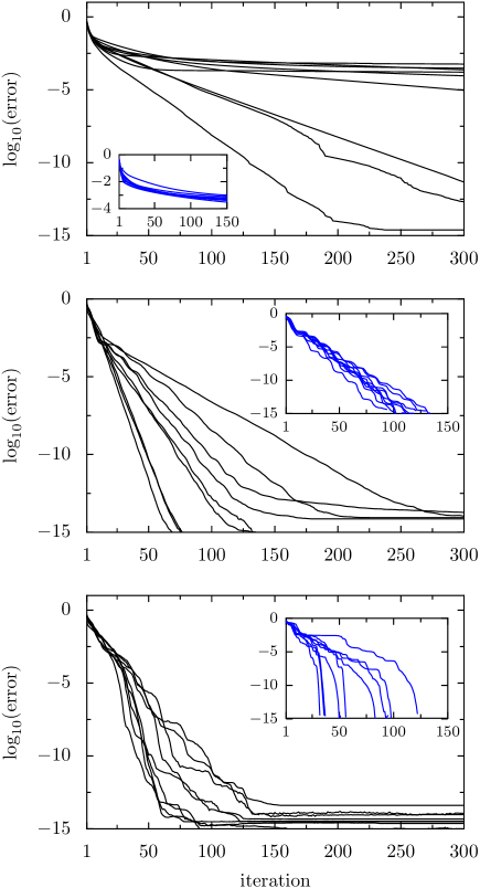
Figure 1: (color online). Convergence plots of the algorithms used to evaluate the entanglement of formation on ten random full-rank two-qubit states (each plot was done using the same ten states) showing the difference between the numerical data and the analytical result as a function of the iteration number. Top: The modified steepest descent algorithm from Ref. Manton (2002); Middle: The generalized conjugate gradient method from Sec. III.1; Bottom: Quasi-Newton on the parameterized search space, Sec. III.2. Each curve in the main plot is averaged over ten randomly chosen initial points. The typical behavior of the algorithms for a single fixed density matrix, but with varying initial points of the iteration, is displayed in the insets.

The entanglement of formation Bennett et al. (1996a) is a popular entanglement measure for bipartite mixed states. It is defined as the convex roof of the entropy of entanglement Bennett et al. (1996b), which is, for a state $|\psi\rangle$, the von-Neumann entropy $S(\rho)=-\mathop{\mathrm{missing}}{Tr}\nolimits\rho\log_{2}\rho$ of the reduced density matrix $\rho=\mathop{\mathrm{missing}}{Tr}\nolimits_{B}|\psi\rangle\langle\psi|$, $\mathop{\mathrm{missing}}{Tr}\nolimits_{B}$ denoting the partial trace over the second subsystem.

Figure 1 shows the convergence behavior of the algorithms applied to ten random full-rank two-qubit density matrices. Displayed is the error at each step of the iteration between the respective iteration value and the true result. The latter is known analytically from Ref. Wootters (1998).

Compared to the algorithms described here, the modified steepest descent algorithm due to Ref. Manton (2002) (top panel) performs rather poorly. We are aware of the fact that we are comparing here a steepest descent algorithm with two superlinear algorithms. However, apart from presenting convergence properties, we would like to point out that the modified steepest descent algorithm often converges to imprecise solutions, i.e., it gets stuck in undesirable local minima. Rather than on the starting point, this phenomenon seems to depend more on the actual density matrix itself.

The conjugate gradient algorithm due to Ref. Audenaert et al. (2001) (middle panel) also shows some dependence on the form of the density matrix, but always reaches satisfactory accuracy. The results for the parameterized quasi-Newton method (bottom panel) do not, at first glance, show the typical fast drop to the solution when close to a good local minimum. This is due to the effect that changing the starting point seems to have more influence on the number of required iterations in the case of the quasi-Newton method (see insets in Fig. 1). When considering single (non-averaged) runs of the algorithm, the fast convergence to the minimum becomes visible. In conclusion, the conjugate gradient and the parameterized quasi-Newton methods perform best in this case, the latter even slightly better than the former.

III.3.2 Tangle of GHZ/W mixtures

The second test case we present here is concerned with the evaluation of the tangle of the rank-2 mixed states

$$\rho(\eta)=\eta|\mathrm{GHZ^{+}_{3}}\rangle\langle\mathrm{GHZ^{+}_{3}}|+(1-\eta)|\mathrm{W}\rangle\langle\mathrm{W}|,$$ (38)

where $|\mathrm{GHZ}^{+}_{3}\rangle$ has been defined in Eq. (1),

$$|\mathrm{W}\rangle=\frac{1}{\sqrt{3}}\big{(}|{\uparrow\downarrow\downarrow}\rangle+|{\downarrow\uparrow\downarrow}\rangle+|{\downarrow\downarrow\uparrow}\rangle\big{)}$$ (39)

is the three-qubit W state Dür et al. (2000), and $0\leq\eta\leq 1$. The tangle $\tau_{p}$ Coffman et al. (2000) is an entanglement measure for pure states of three qubits and is known to be an entanglement monotone Dür et al. (2000). It can hence be generalized to mixed states by the convex roof construction (2). We will denote the mixed-state tangle by $\tau$, in contrast to the pure-state version $\tau_{p}$. The definition of $\tau_{p}$ reads

$$\tau_{p}(|\psi\rangle)=4\ |d_{1}-2d_{2}+4d_{3}|,$$ (40)

where

$$d_{1} = \psi^{2}_{1}\psi^{2}_{8}+\psi^{2}_{2}\psi^{2}_{7}+\psi^{2}_{3}\psi^{2}_{6}+\psi^{2}_{5}\psi^{2}_{4},$$ (41)

$$d_{2} = \psi_{1}\psi_{8}\psi_{4}\psi_{5}+\psi_{1}\psi_{8}\psi_{6}\psi_{3}+\psi_{1}\psi_{8}\psi_{7}\psi_{2}+\psi_{4}\psi_{5}\psi_{6}\psi_{3}$$ (42)

$$\;\;+\psi_{4}\psi_{5}\psi_{7}\psi_{2}+\psi_{6}\psi_{3}\psi_{7}\psi_{2},$$

$$d_{3} = \psi_{1}\psi_{7}\psi_{6}\psi_{4}+\psi_{8}\psi_{2}\psi_{3}\psi_{5},$$ (43)

and $\psi_{1},\psi_{2},\ldots,\psi_{8}$ denote the components of the state $|\psi\rangle$ represented in an arbitrary product basis. In this form, the derivatives of $\tau_{p}$ with respect to the real and imaginary parts of the components of $|\psi\rangle$, as required by the gradient Eqs. (10, 11), can be read off most easily. The tangle takes values between $0$ and $1$ and is maximal for GHZ states. The tangle of the states $\rho(\eta)$ has been studied in Ref. Lohmayer et al. (2006), where analytical expressions as a function of $\eta$ where presented. Particularly, it was found that the tangle vanishes for all $0\leq\eta\leq\eta_{0}$, where $\eta_{0}=\frac{4\sqrt[3]{2}}{3+4\sqrt[3]{2}}\approx 0.6269$, and then continuously increases to unity at $\eta=1$.

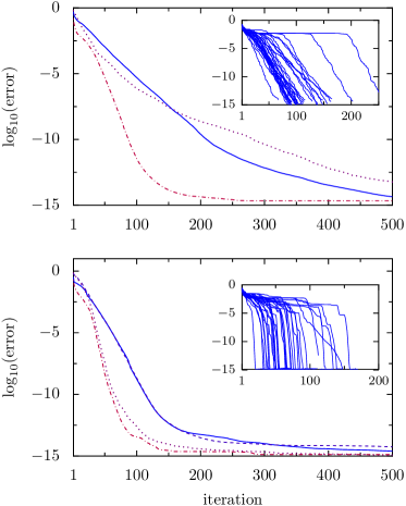
Figure 2: (color online). Convergence of the generalized conjugate gradient (top) and the parameterized quasi-Newton (bottom) algorithms for the tangle of GHZ/W states Eq. (38). The curves for the values $\eta=\frac{1}{5}\eta_{0}$ (solid line), $\eta=(1-10^{-4})\eta_{0}$ (dashed line), $\eta=(1+10^{-4})\eta_{0}$ (dotted line), and $\eta=\frac{7}{5}\eta_{0}$ (dashed-dotted line) have each been obtained by averaging 100 successful runs starting with random initial points. The typical behavior of single runs is shown in the insets, where the 100 successful tries that yield one curve in the main plots are displayed.

In Figure 2 we plot the error between the numerically obtained and analytically calculated values of $\tau(\rho(\eta))$ as a function of the iteration number for four particular values of $\eta$ (see caption of the figure). Only the results of the generalized conjugate gradient (top panel) and the parameterized quasi-Newton (bottom panel) method are shown. The modified steepest descent algorithm from Ref. Manton (2002) did not succeed to converge to a reasonable local minimum for the lowest three values of $\eta$ considered. In these cases, we empirically find the success rate, which we define as the relative number of final errors smaller than $10^{-6}$, to be $\lesssim 0.1\%$. For the largest value of $\eta$ examined, the algorithm showed typical linear convergence behavior and arrived at a precision around $10^{-12}-10^{-6}$ after $1000$ iterations with a rather high success rate of about $60\%$. Similarly, the generalized conjugate gradient algorithm failed to obtain reasonable results for the value of $\eta$ slightly below the threshold value $p_{0}$ in most attempts, and we find a success rate of $\lesssim 0.2\%$. The success probability for the other three values of $\eta$ are between $12\%$ and $95\%$, whereas they are between $25\%$ and $80\%$ for the parameterized quasi-Newton algorithm. One can see, with the help of looking more detailed into the behavior of single runs (see insets), that the averaged convergence plots are slightly flattened out due to some rather rare occurrences of slow convergence. Still, one can observe that the parameterized quasi-Newton method converges faster to good local minima.

III.4 Local unitary equivalence

We would like to remark here that the parameterized quasi-Newton method is also capable of determining whether two arbitrary mixed states are equivalent up to local unitary transformations. While this problem has an operational solution in some special cases (see, e.g., Ref. Fei and Jing (2005) and references therein), there is no generally applicable operational criterion known capable of making this decision. Using the parametrization developed in Sec. III.2, one can express each local unitary transformation $U_{i}$ in the matrix $U=U_{1}\otimes U_{2}\otimes\ldots\otimes U_{n}$ by its Euler-Hurwitz angles and optimize over the whole set of all angles simultaneously. Furthermore, on can study in this way how ‘close’ two mixed state are with respect to local unitary equivalence. Note that such kind of analyses are not possible with the modified steepest descent or the generalized conjugate gradient methods, since, as there is no parametrization, one can optimize over only one unitary matrix at a time.

IV Physical Application

In this section, we use the algorithms developed and described above to evaluate a multipartite mixed-state entanglement measure of a concrete physical system.

IV.1 Exchange-coupled spin rings with inhomogeneous magnetic field geometry

In the following, we consider the Hamiltonian

$$H=-J\sum_{i=1}^{N}\mathbf{S}_{i}\cdot\mathbf{S}_{i+1}+b\sum_{i=1}^{N}(S_{i}^{x}\cos\alpha_{i}+S_{i}^{y}\sin\alpha_{i}),$$ (44)

where $\mathbf{S}_{i}=(S_{i}^{x},S_{i}^{y},S_{i}^{z})$, $S_{i}^{k}=\sigma^{k}/2$ with $\sigma^{k}$ being the standard Pauli matrices acting on the $i$th spin, $\mathbf{S}_{N+1}\equiv\mathbf{S}_{1}$ and the angles $\alpha_{k}=2\pi(k-1)/N$, $k=1,\ldots,N$. Equation (44) describes a closed ring of $N\geq 2$ equidistant exchange-coupled spin qubits with local in-plane magnetic fields $\mathbf{b}_{i}\equiv(b\cos\alpha_{i},b\sin\alpha_{i},0)^{T}$ which are chosen such that the system is invariant under rotations by multiples of $2\pi/N$ about the center of the ring. The exchange coupling $J$ is throughout assumed to be ferromagnetic (i.e., $J>0$). The fields in Eq. (44) are chosen to point radially outwards, but the following discussion and results also hold for any other local in-plane field configuration possessing the same rotational symmetry, since all these systems are local unitary equivalents. The system is depicted schematically in Fig. 3 (a) for three spins.

In fact, we are considering here a generalization of one of the $N=3$ cases studied in Ref. Röthlisberger et al. (2008). There, the particular field configuration resulted from semiclassical considerations with the goal of obtaining a state which is close to a GHZ state [see Eq. (1)] as the ground state of the system. In that case, entanglement can be created by merely cooling the system to low enough temperatures. In principle, the argumentation for the occurrence of a GHZ ground state presented in Ref. Röthlisberger et al. (2008) can be extended to a number of qubits $N>3$. However, it can be expected that for $N\rightarrow\infty$, the lowest-lying multiplet becomes a continuous spectrum. Hence, the question arises up to which numbers of spins $N$ this setup still allows generating GHZ-type entanglement. Before further investigating this question, we briefly restate the arguments of Ref. Röthlisberger et al. (2008) for the convenience of the reader.

We start from the fact that in the ground state of the classical analog of the Hamiltonian (44), all spins are aligned for $b=0$. However, no direction of alignment is favored, reflecting the full rotational symmetry of the system in spin space. Small local magnetic fields ($b\ll J$), applied in the way described above, break this symmetry and one is left with the two degenerate ground states $\uparrow\uparrow\ldots\uparrow$ and $\downarrow\downarrow\ldots\downarrow$ where the representation (’quantization’) axis is the usual $z$-direction. In fact, each spin is slightly tilted against its local magnetic field, but there is no globally favored direction of orientation, such as with, e.g., a global spatially uniform magnetic field. Note that this effect of tilting vanishes as $b\rightarrow 0$. Due to the Zeeman term in Eq. (44) there is an energy barrier between any path connecting the two degenerate minima. In the quantum case, tunneling through this barrier lifts the degeneracy between the ground states and one obtains a tunnel doublet. Thus, in the limit $b\rightarrow 0^{+}$, the two lowest lying states are the generalized GHZ states given in Eq. (1).

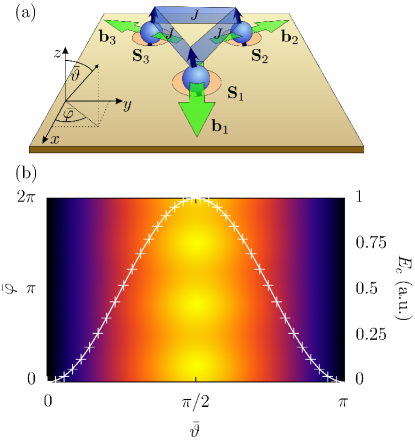
Figure 3: (color online). (a) Schematic depiction of the system described by the Hamiltonian (44) for $N=3$. Three spins $\mathbf{S}_{i}$ are situated at the corners of an equilateral triangle and are ferromagnetically exchange-coupled with coupling strength $J$. Local radial in-plane magnetic fields $\mathbf{b}_{i}$ (shown as green arrows in the $xy$-plane) point radially outwards. As discussed in the text, any other in-plane field geometry obeying the same radial symmetry (such as, e.g., a ‘chiral’ field looping around the triangle) leads to equivalent results. (b) Classical energy surface $E_{c}$ of the system shown in the top panel. The ‘mean’ angles $\bar{\vartheta}$ and $\bar{\varphi}$ (introduced in the top panel) are well suited to characterize the state of the system since fluctuations around these angles are small for $b\ll J$ and sum to zero. The superimposed white line shows the perturbatively calculated energy barrier at $\bar{\varphi}=\pi/2$ [see Eq. (2) in Ref. Röthlisberger et al. (2008)], whereas the crosses are due to a corresponding numerical minimization of the energy.

As an illustration, we plot the energy surface of the classical three-spin system corresponding to Eq. (44) in Fig. 3 (b). We have previously argued [see Ref. Röthlisberger et al. (2008), especially the discussion leading to Eq. (2) therein] that this energy can be expressed in terms of two ‘mean’ spherical angles $\bar{\varphi}$ and $\bar{\vartheta}$ [cf. Fig. 3 (a)], since all spins will basically align in the present limit $b\ll J$, up to small fluctuations which sum to zero and are chosen to minimize the total energy. One can nicely see how the out-of-plane configurations at $\bar{\vartheta}=0$ and $\bar{\vartheta}=\pi$ are energetically favored. For any value of $\bar{\varphi}$, a path connecting the two minima has to overcome an energy barrier which scales as $O(b^{2})$. In the figure, this barrier is displayed by the superimposed white line for the specific value $\bar{\varphi}=\pi/2$.

Independently of $N$, we are generally confronted with the following problem if we want to achieve the systems considered here to be in a highly entangled state at non-zero temperature. On the one hand, the energy splitting between the ground state and the first excited state vanishes as $b$ goes to zero. On the other hand, a perfect GHZ state is obtained exactly in this limit. For increasing magnetic field, the states continuously deviate from the maximally entangled GHZ state, as can be imagined with the help of the classical picture, where the spins start to tilt. One therefore has to choose the strength of $b$ as a tradeoff between having a highly entangled ground state and separating this state in energy from the next higher state.

In order to find this optimal magnetic field strength at a given temperature $T\neq 0$ we evaluate a suited mixed-state entanglement measure on the system’s canonical density matrix $\rho=\exp(-\beta H)/\mathop{\mathrm{missing}}{Tr}\nolimits\exp(-\beta H)$ where $\beta=1/k_{\mathrm{B}}T$ and $k_{\mathrm{B}}$ is Boltzmann’s constant. When we studied the case $N=3$ in Ref. Röthlisberger et al. (2008) we used the tangle [see Eq. (40)] as our pure-state measure of choice, since it is an entanglement measure for three qubits. The generalization to mixed states was done via the convex-roof construction Eq. (2). Here, however, we need a pure-state entanglement measure which is defined for any $N\geq 2$.

IV.2 Entanglement measure

In principle, an exponentially increasing number of distinct entanglement measures is required to capture all possible quantum correlations in a general pure state of $N$ qudits. This may be viewed as the reason for the rather large number of proposals for multipartite entanglement measures that have been put forward over the last years. Various insights about the structure and characterization of multipartite entanglement have been gained by studying such measures. For our purpose, we want to have a measure that is easy (and fast) to compute (in particular, that is an analytic function whose complexity grows at most polynomially with $N$), that captures the type of entanglement present in our system well, and that possibly has a nice (physical) interpretation. We found that the Meyer-Wallach measure Meyer and Wallach (2002), defined for an arbitrary number of qubits, fulfills all these criteria. According to Ref. Brennen (2003), it can be written in the compact form

$$\gamma(|\psi\rangle)=2\left[1-\frac{1}{N}\sum_{k=1}^{N}\mathop{\mathrm{missing}}{Tr}\nolimits(\rho_{k}^{2})\right],$$ (45)

where $\rho_{k}$ is the density matrix obtained by tracing out all but the $k$th qubit out of $|\psi\rangle\langle\psi|$. This is simply the subsystem linear entropy averaged over all bipartite partitions involving one qubit and the rest Footnote2 . Moreover, it was shown that this entanglement measure is experimentally observable by determining a set of parameters that grows linearly with $N$, in contrast to the exponentially increasing complexity of quantum state tomography Brennen (2003). We note at this point that the Meyer-Wallach entanglement has been generalized to a broader family of entanglement measures Scott (2004) that might give deeper insight into the structure of multipartite entanglement. However, we stick to the simple form (45) for our numerical calculations, as this measure turns out to describe our type of entanglement well.

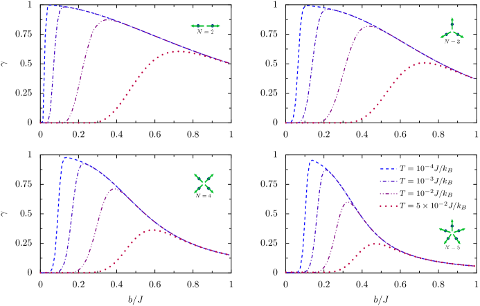
Figure 4: (color online). Meyer-Wallach entanglement measure for the system described by the Hamiltonian Eq. (44) at different temperatures for several numbers of particles. Concretely, the cases $N=2$ (top left), $N=3$ (top right), $N=4$ (bottom left), and $N=5$ (bottom right) are studied at temperatures $T=10^{-4}J/k_{\mathrm{B}}$ (dashed line), $T=10^{-3}J/k_{\mathrm{B}}$ (dashed-dotted line), $T=10^{-2}J/k_{\mathrm{B}}$ (dashed-dot-dotted line), and $T=5\times 10^{-2}J/k_{\mathrm{B}}$ (dotted line).

The Meyer-Wallach measure is an entanglement monotone (and can thus be extended to mixed states via the convex-roof construction), lies between zero and one, vanishes only for full product states (i.e., states of the form $|\psi\rangle=\bigotimes_{i}|\psi_{i}\rangle,i=1,\ldots,N$), and is maximal for generalized GHZ states Eq. (1). The upper bound is however also reached by other states, for instance by the so-called cluster states Brennen (2003); Briegel and Raussendorf (2001). A drawback of the Meyer-Wallach measure is that it can also be maximized by partially separable states. For example, the state $|\Psi\rangle=|\Phi\rangle\otimes|\Phi\rangle$, where $|\Phi\rangle=(|{\uparrow\uparrow}\rangle+|{\downarrow\downarrow}\rangle)/\sqrt{2}$ is a bipartite Bell state, gives $\gamma(|\Psi\rangle)=1$ although it is clearly not globally entangled Brennen (2003). This is however not a problem in our study for two reasons. First of all, we can check by numerical diagonalization that the ground state of our systems indeed converges to a multiparite GHZ state (at least for the first few $N\lesssim 20$). Secondly, comparing the data for $N=3$ with our earlier study in Ref. Röthlisberger et al. (2008) where we had employed the tangle, we find the same qualitative behavior of both entanglement measures. Moreover, the optimal values of $b$ for which the measures reach their maxima at a given temperature coincide almost perfectly. It is thus reasonable to assume that the Meyer-Wallach entanglement measure is well suited for quantifying entanglement in our systems.

The numerical evaluation of the Meyer-Wallach measure extended to mixed states via the convex-roof construction requires the derivatives of $\gamma(|\psi\rangle)$ with respect to the real and imaginary components of $|\psi\rangle$ [see Eqs. (10, 11)]. Due to the partial traces, these expressions are a bit cumbersome. However, exploiting the rotational symmetry of the Hamiltonian studied here, they can be considerably simplified (see Appendix).

IV.3 Results

Before we present and discuss our numerical results, we would like to mention that studying the system Eq. (44) analytically for arbitrary $N$ is rather difficult. An exact diagonalization of the Hamiltonian is not known for arbitrary $N$, and perturbation theory to constant order in $b$ (independent of $N$) is not suitable to study the ground-state properties of the system, since the ground-state splitting is lifted only in $N$-th order. One can can thus generally expect that the ground-state splitting scales with the number of spins as $b^{N}$. Since we must always have $b\ll 1$, this goes to zero for large $N$, as discussed in Sec. IV.1 above. Obtaining highly entangled states at finite temperature with this approach will thus be increasingly difficult for an increasing number of spins $N$.

Our numerical results are presented in Figs. 4 and 5. Figure 4 shows the Meyer-Wallach measure for $N=2,3,4$, and $5$ spins at four different temperatures (see caption of the figure). Each data point is the result of whichever of the two algorithms described in Sec. III performed better in a few trials with random initial conditions.

For a fixed number of spins, the entanglement as a function of the magnetic field strength $b$ assumes a maximum. This maximal entanglement $\gamma_{\mathrm{max}}(T)$ is increased and its position is shifted to smaller magnetic field values as the temperature is lowered. This is due to the fact that at low temperatures, only a small magnetic field is required in order to make the ground-state splitting sufficiently large compared with temperature. Since these small field values only slightly disturb the ideal GHZ configuration, almost maximal values of the entanglement measure (corresponding to almost perfect GHZ-states) are observed. With higher temperature, larger field values are required to protect the ground state. Consistent with the semiclassical picture, this perturbs the desired spin configuration and leads to a lower amount of entanglement. For large magnetic fields, all curves coincide eventually, as the system is always found in the ground state in that case.

Figure 5 gives more insight into the dependence of maximal entanglement $\gamma_{\mathrm{max}}(T)$ on temperature and the number of particles. The plot was obtained by maximizing the Meyer-Wallach measure over the magnetic field strength $b$ while holding the temperature fixed. Displayed is the difference between the resulting data to the zero-temperature maximum (being equal to $1$) as a function of temperature for different numbers of particles (see caption of the figure). Clearly, the maximally achievable entanglement $\gamma_{\mathrm{max}}(T)$ decreases for both increasing temperature and increasing number of particles. The qualitative dependence on the temperature was discussed already above. Here we additionally see an almost linear behavior on a log-log scale at low temperatures, suggesting a power-law decay of the maximal entanglement of the form $1-\gamma_{\mathrm{max}}(T)\propto T^{\alpha}$ with an exponent $\alpha$ depending on the number of particles $N$.

The decrease of $\gamma_{\mathrm{max}}(T)$ with the number of spins $N$ at fixed temperature is due to the fact that the energy splitting between the ground and first excited state scales as $b^{N}$. With a larger number of particles, a higher magnetic field is required to achieve a sufficiently large splitting. This in turn lowers the entanglement in the ground state, due to its $b$-dependence, resulting in a lowered maximum of the Meyer-Wallach measure. As an additional obstacle, the ground-state entanglement as a function of $b$ decays even more rapidly as the number of particles is increased. This can be seen from the inset of figure 5, where, at $T=0$, the $b$-values yielding the Meyer-Wallach measure $0.5$ (full width at half maximum, since the maximum at $T=0$ is always $1$) are shown as a function of $N$.

V conclusions

We have presented two ready-to-use numerical algorithms to evaluate any generic convex-roof entanglement measure. While one is based on a conjugate gradient algorithm operating directly on the search space, the other one is a quasi-Newton procedure performing the search in the transformed unconstrained Euclidean space. All required formulas to implement either of the two algorithms have been stated explicitly, which, in order to calculate different convex-roof extended pure-state measures, merely leaves the user with the task of calculating its derivatives with respect to the real and imaginary components of the pure-state argument. The relatively different nature of the two procedures increases the chances that at least one of them performs well in the concrete application. In a series of numerical tests, we have found that the algorithms perform well and especially significantly better than previously presented (non Newton-type) ready-to-use optimization problems on the Stiefel manifold. However, it is found that the convergence properties, as is often the case in involved optimization problems, depend on the cost function. This suggests to try applying different techniques to a particular optimization problem and examine which one performs best in that case.

Further, we have applied our algorithms to evaluate a multipartite entanglement measure on density matrices originating from a real physical system. The latter consists of $N$ ferromagnetically exchange-coupled spin-$\frac{1}{2}$ particles placed on the edges of a regular polygon with $N$ edges. We have argued that a particular local magnetic field geometry, namely radially symmetric in-plane fields, favor a highly entangled ground state configuration. We have confirmed this argumentation by evaluating the mixed-state Meyer-Wallach entanglement measure, defined for an arbitrary number of qubits, and found indeed high values of entanglement at low temperatures and specific magnetic field strengths. This not only quantifies the entanglement properties present in this system, but also serves more generally as a proof-of-principle for the usefulness and applicability of our algorithms.

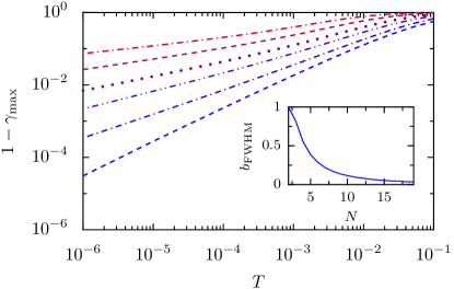
Figure 5: (color online). Difference between zero-temperature and finite-temperature maximally achievable Meyer-Wallach entanglement measure as a function of temperature for systems with $N=2,3,4,5,7,10$ spins (from bottom to top). Inset: Value of the magnetic field strength $b$ as a function of system size at which the ground state yields the Meyer-Wallach value 0.5 (full width at half maximum).

*

Appendix A Derivatives of the Meyer-Wallach entanglement measure

Within our numerical framework, the evaluation of the Meyer-Wallach measure $\gamma(|\psi\rangle)$ [see Eq. (45)] requires its partial derivatives with respect to the real and imaginary components of $|\psi\rangle$ [see Eqs. (10, 11)]. They are given by

$$\left.\frac{\partial\gamma}{\partial\mathop{\mathrm{missing}}{Re}\psi^{(i)}}\right|_{|\psi\rangle} =-\frac{8}{N}\sum_{k=1}^{N}\sum_{\mu=0}^{1}\sum_{\nu_{1}=0}^{1}\sum_{\nu_{2}=0}^{1}\cdots\sum_{\nu_{N}=0}^{1}\mathop{\mathrm{missing}}{Re}\left(\psi^{(\nu_{1},\nu_{2},\ldots,\nu_{k-1},\mu,\nu_{k+1},\ldots,\nu_{N})}\rho_{k}^{\nu_{k},\mu}\right),$$ (46)

$$\left.\frac{\partial\gamma}{\partial\mathop{\mathrm{missing}}{Im}\psi^{(i)}}\right|_{|\psi\rangle} =-\frac{8}{N}\sum_{k=1}^{N}\sum_{\mu=0}^{1}\sum_{\nu_{1}=0}^{1}\sum_{\nu_{2}=0}^{1}\cdots\sum_{\nu_{N}=0}^{1}\mathop{\mathrm{missing}}{Im}\left(\psi^{(\nu_{1},\nu_{2},\ldots,\nu_{k-1},\mu,\nu_{k+1},\ldots,\nu_{N})}\rho_{k}^{\nu_{k},\mu}\right).$$ (47)

Here, we represented the $i$th component of $|\psi\rangle$ by the tuple $i=(\nu_{1},\ldots,\nu_{N})$, with the indices $\nu_{j}\in\{0,1\}$ corresponding to some arbitrary product basis $\{|\nu_{1}\rangle|\nu_{2}\rangle\cdots|\nu_{N}\rangle\}_{\nu_{j}=0}^{1}$ of the spin system. Furthermore, $\rho_{k}^{\nu,\mu}$ denotes the matrix element with indices $(\nu,\mu)$ of the reduced density matrix $\rho_{k}=\mathop{\mathrm{missing}}{Tr}\nolimits_{\nu_{1},\nu_{2},\ldots,\nu_{k-1},\nu_{k+1},\ldots,\nu_{N}}|\psi\rangle\langle\psi|\in\mathds{C}^{2\times 2}$.

In case of the systems studied in Sec. IV.1, the computation of the Meyer-Wallach measure (45) and its derivatives can be greatly simplified by exploiting the rotational symmetry of the Hamiltonian $H$. Since we have $[H,\mathcal{R}]=0$, where $\mathcal{R}$ is the symmetry operator for the rotation by an angle of $2\pi/N$ about the central axis perpendicular to the plane of the spin ring, all $\rho_{k}$ in Eq. (45) are unitary equivalents for a simultaneous eigenstate $|\psi\rangle$ of $H$ and $\mathcal{R}$. This reduces Eq. (45) to the simple form

$$\gamma(|\psi\rangle)=2[1-\mathop{\mathrm{missing}}{Tr}\nolimits(\rho_{1}^{2})].$$ (48)

The corresponding derivatives read

$$\left.\frac{\partial\gamma}{\partial\mathop{\mathrm{missing}}{Re}\psi^{(i)}}\right|_{|\psi\rangle} =-8[\rho_{1}^{0,0}\mathop{\mathrm{missing}}{Re}\psi^{(i)}+\mathop{\mathrm{missing}}{Re}(\rho_{1}^{0,1}\psi^{(2^{N-1}+i)})],$$ (49)

$$\left.\frac{\partial\gamma}{\partial\mathop{\mathrm{missing}}{Im}\psi^{(i)}}\right|_{|\psi\rangle} =-8[\rho_{1}^{0,0}\mathop{\mathrm{missing}}{Im}\psi^{(i)}+\mathop{\mathrm{missing}}{Im}(\rho_{1}^{0,1}\psi^{(2^{N-1}+i)})],$$ (50)

for $0\leq i\leq 2^{N-1}-1$, and

$$\left.\frac{\partial\gamma}{\partial\mathop{\mathrm{missing}}{Re}\psi^{(i)}}\right|_{|\psi\rangle} =-8[\rho_{1}^{1,1}\mathop{\mathrm{missing}}{Re}\psi^{(i)}+\mathop{\mathrm{missing}}{Re}(\rho_{1}^{0,1}\psi^{\ast(i-2^{N-1})})],$$ (51)

$$\left.\frac{\partial\gamma}{\partial\mathop{\mathrm{missing}}{Im}\psi^{(i)}}\right|_{|\psi\rangle} =-8[\rho_{1}^{1,1}\mathop{\mathrm{missing}}{Im}\psi^{(i)}-\mathop{\mathrm{missing}}{Im}(\rho_{1}^{0,1}\psi^{\ast(i-2^{N-1})})],$$ (52)

for $2^{N-1}\leq i\leq 2^{N}-1$. In practice, we first diagonalize $H$ numerically Footnote3 , subsequently diagonalize further any degenerate spaces with respect to $\mathcal{R}$, and then apply the simplified formulas above.

References

- Schrödinger (1935) E. Schrödinger, Naturwissenschaften 23, 823 (1935).
- Einstein et al. (1935) A. Einstein, B. Podolsky, and N. Rosen, Phys. Rev. 47, 777 (1935).
- Nielsen and Chuang (2000) M. A. Nielsen and I. L. Chuang, Quantum Computation and Quantum Information (Cambridge University Press, New York, 2000).
- Deutsch and Jozsa (1992) D. Deutsch and R. Jozsa, Proc. R. Soc. London, Ser. A 439, 553 (1992).
- Cleve et al. (1998) R. Cleve, A. Ekert, C. Macchiavello, and M. Mosca, Proc. R. Soc. London, Ser. A 454, 339 (1998).
- Grover (1996) L. K. Grover, in Proceedings, 28th Annual ACM Symposium on the Theory of Computing (1996), p. 212.
- Shor (1997) P. Shor, SIAM Journal on Computing 26, 1484 (1997).
- Plenio and Virmani (2007) M. B. Plenio and S. Virmani, Quant. Inf. Comp. 7, 1 (2007).
- Bell (1964) J. Bell, Physics 1, 195 (1964).
- Ursin et al. (2007) R. Ursin, F. Tiefenbacher, T. Schmitt-Manderbach, H. Weier, T. Scheidl, M. Lindenthal, B. Blauensteiner, T. Jennewein, J. Perdigues, P. Trojek, et al., Nature Phys. 3, 481 (2007).
- Horodecki et al. (1996) M. Horodecki, P. Horodecki, and R. Horodecki, Phys. Lett. A 223, 1 (1996).
- Terhal (2000) B. Terhal, Phys. Lett. A 271, 319 (2000).
- Emary and Beenakker (2004) C. Emary and C. W. J. Beenakker, Phys. Rev. A 69, 032317 (2004).
- Gühne et al. (2007) O. Gühne, M. Reimpell, and R. F. Werner, Phys. Rev. Lett. 98, 110502 (2007).
- Eisert et al. (2007) J. Eisert, F. G. S. L. Brandão, and K. M. R. Audenaert, New J. Phys. 9, 46 (2007).
- Bennett et al. (1996a) C. H. Bennett, D. P. DiVincenzo, J. A. Smolin, and W. K. Wootters, Phys. Rev. A 54, 3824 (1996a).
- Coffman et al. (2000) V. Coffman, J. Kundu, and W. K. Wootters, Phys. Rev. A 61, 052306 (2000).
- Mintert et al. (2005a) F. Mintert, M. Kuś, and A. Buchleitner, Phys. Rev. Lett. 95, 260502 (pages 4) (2005a).
- Meyer and Wallach (2002) D. A. Meyer and N. R. Wallach, J. Math. Phys. 43, 4273 (2002).
- Uhlmann (2000) A. Uhlmann, Phys. Rev. A 62, 032307 (2000).
- Audenaert et al. (2001) K. Audenaert, F. Verstraete, and B. De Moor, Phys. Rev. A 64, 052304 (2001).
- Röthlisberger et al. (2008) B. Röthlisberger, J. Lehmann, D. S. Saraga, P. Traber, and D. Loss, Phys. Rev. Lett. 100, 100502 (2008).
- Greenberger et al. (1989) D. M. Greenberger, M. Horne, and A. Zeilinger, Bell’s Theorem, Quantum Theory, and Conceptions of the Universe (Kluwer Academic Publishers, Dortrecht, 1989).
- Mintert et al. (2005b) F. Mintert, A. R. R. Carvalho, M. Kuś, and A. Buchleitner, Phys. Rep. 415, 207 (2005b).
- Hughston et al. (1993) L. P. Hughston, R. Jozsa, and W. K. Wootters, Phys. Lett. A 183, 14 (1993).
- Kirkpatrick (2005) K. A. Kirkpatrick, Found. Phys. Lett. 19, 95 (2005).
- Absil et al. (2008) P.-A. Absil, R. Mahony, and R. Sepulchre, Optimization Algorithms on Matrix Manifolds (Princeton University Press, Princeton, New Jersey, 2008).
- Edelman et al. (1998) A. Edelman, T. A. Arias, and S. T. Smith, SIAM J. Matrix Anal. Appl. 20, 303 (1998).
- Manton (2002) J. H. Manton, IEEE Trans. Signal Process. 50, 635 (2002).
- Wootters (1998) W. K. Wootters, Phys. Rev. Lett. 80, 2245 (1998).
- Press et al. (1992) W. H. Press, S. A. Teukolsky, W. T. Vetterling, and B. P. Flannery, Numerical Recipes in C: The Art of Scientific Computing (Cambridge University Press, New York, NY, USA, 1992).
- Nocedal and Wright (1999) J. Nocedal and S. J. Wright, Numerical Optimization (Springer, 1999).
- Euler (1987) L. Euler, in Opera Omnia, series I, vol. VI (Birkhäuser, Basel, 1987).
- Hurwitz (1933) A. Hurwitz, in Mathematische Werke, vol. II (Birkhäuser, Basel, 1933).
- Terhal et al. (2002) B. M. Terhal, M. Horodecki, D. W. Leung, and D. P. DiVincenzo, J. Math. Phys. 43, 4286 (2002).
- Golub and Van Loan (1996) G. H. Golub and C. F. Van Loan, Matrix Computations (Johns Hopkins University Press, Baltimore, 1996).
- (37) Allowing the iteration points to move outside of may result in large absolute values of the angles, possibly leading to reduced precision in the output. Such effects can be prevented by projecting the current iteration point back to a few times in the first couple of iterations.
- Bennett et al. (1996b) C. H. Bennett, H. J. Bernstein, S. Popescu, and B. Schumacher, Phys. Rev. A 53, 2046 (1996b).
- Dür et al. (2000) W. Dür, G. Vidal, and J. I. Cirac, Phys. Rev. A 62, 062314 (2000).
- Lohmayer et al. (2006) R. Lohmayer, A. Osterloh, J. Siewert, and A. Uhlmann, Phys. Rev. Lett. 97, 260502 (2006).
- Fei and Jing (2005) S.-M. Fei and N. Jing, Physics Letters A 342, 77 (2005).
- Brennen (2003) G. K. Brennen, Quant. Inf. Comp. 3, 619 (2003).
- (43) The subsystem linear entropy , where , is a well-established bipartite entanglement measure that is often used instead of the von-Neumann entropy in order to simplify calculations Scott (2004).
- Scott (2004) A. J. Scott, Phys. Rev. A 69, 052330 (2004).
- Briegel and Raussendorf (2001) H. J. Briegel and R. Raussendorf, Phys. Rev. Lett. 86, 910 (2001).
- (46) Since for the number of particles considered in Sec. IV.3 the splitting between the lowest and the next higher mutliplet is still always large compared with temperature, we diagonalize only the lowest-lying -dimensional subspace of using a Lanczos algorithm.