A Type System for Parallel Components

Abstract

The # component model was proposed to improve the practice of parallel programming. This paper introduces a type system for # programming systems, aiming to lift the abstraction and safety of programming for parallel computing architectures by introducing a notion of abstract component based on universal and existential bounded quantification. Issues about the implementation of such type system in HPE, a # programming system, are also discussed.

1 Introduction

Multi-core processors have already made parallel computing a mainstream technology, but high performance computing (HPC) applications that run on clusters and grids have already attracted the investments of the software industry. The key for reaching peak performance is the knowledge of how to apply HPC techniques for parallel programming by looking at the particular features of the parallel computing architecture.

With the raising of complexity and scale of HPC applications [Post and Votta 2005], HPC developers now demands for software engineering artifacts to develop HPC software [Sarkar et al. 2004]. Unfortunately, parallel programming is still hard to be incorporated into usual software development platforms [Bernholdt D. E. et al. 2004]. Due to the success of component technologies in the commercial scenario, component models and frameworks for HPC applications have been proposed [van der Steen 2006], such as CCA and its compliant frameworks [Armstrong et al. 2006], Fractal/ProActive [Bruneton et al. 2002], and GCM [Baude et al. 2008]. However, the HPC community still looks for a general notion of parallel component and better connectors for efficient parallel synchronization.

The # component model was proposed to meet the aims of parallel software in HPC domain. It provides (#-)components with the ability to be deployed in a pool of computing nodes of a parallel execution platform and to address non-functional concerns. Based on a framework architecture recently proposed [Carvalho Junior et al. 2007], a # programming system based on the notion of #-components was designed and prototyped, called HPE (The Hash Programming Environment). This paper presents the design of a type system for # programming systems, adopted in HPE, that support a suitable notion of abstract component for increasing the level of abstraction of parallel programming over particular architectures with minimal performance penalties.

Section 2 presents the # component model and HPE. Section 3 outlines a language for describing configurations of #-components, whose type system is introduced in Section 4 and implemented Section 5. Section 6 concludes this paper, outlining further works.

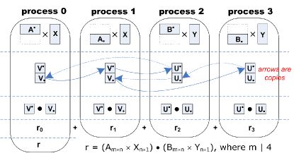
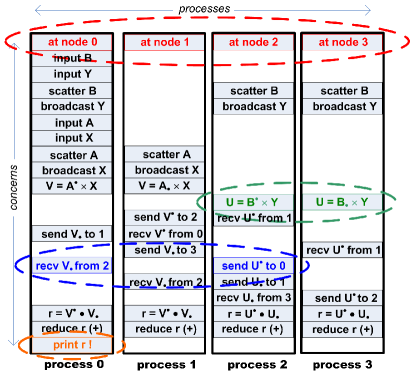
Figure 1: From Processes to #-Components, Intuitively

2 The # Component Model

Notions of parallel components have been proposed in many computational frameworks for HPC applications [van der Steen 2006]. In general, they lack the level of expressiveness and efficiency of message passing libraries such as MPI [Dongarra et al. 1996]. For this reason, the search for more expressive ways to express parallelism with components is at present an important research theme for people that work with CCA (Common Component Architecture), Fractal, and GCM (Grid Component Model) compliant component platforms [Allan et al. 2002, Baude et al. 2007, Baduel et al. 2007]. The # component model proposes a notion of components that are intrinsically parallel and shows how they can be combined to form new components and applications.

A programming system is defined as any artifact for development of programs for applications in some domain. Examples of programming systems are programming languages, problem solving environments, computational frameworks, visual composition languages, and so on. We say that a programming system is component-based if programs are constructed by gluing independent parts that represent some notion of component by means of a set of supported connectors. A component-based programming system complies to the # component model if they support the following features:

• components are built from a set of parts, called units, each one supposed to be deployed in a node of a parallel computing execution platform;

• components can be combined to form new components and applications by means of overlapping composition, a kind of hierarchical composition;

• Each component belongs to one in a finite set of supported component kinds.

Components of # programming systems are called #-components, which has been formally defined in previous works, using category theory and institutions [Carvalho Junior and Lins 2008]. Figure 1 provides an intuitive notion of #-components by assuming the knowledge of the reader about the basic structure of parallel programs, as a set of processes communicating by message passing. For that, it is used a parallel program that calculate $A\times\widehat{x}\bullet B\times\widehat{y}$, where $A_{m{\times}n}$ and $B_{m{\times}k}$ are matrices and $\widehat{x}_{n{\times}1}$ and $\widehat{y}_{k{\times}1}$ are vectors. For that, the parallel program is formed by $N$ processes coordinated in two groups, named $p$ and $q$, with $M$ and $P$ processes, respectively. In Figure 1, $M=P=2$, $p=\{\textbf{process\ 0},\textbf{process\ 1}\}$ and $q=\{\textbf{process\ 2},\textbf{process\ 3}\}$. In the first stage, the processes in $p$ calculate $\widehat{v}=A\times\widehat{x}$, while the processes in $q$ calculate $\widehat{u}=B\times\widehat{y}$, where $\widehat{v}_{m{\times}1}$ and $\widehat{u}_{m{\times}1}$ are intermediate vectors. Figure 1(a) illustrates the partitioning of matrices and vectors and the messages exchanged (arrows). $M^{\bullet}$ denotes the upper rows of the matrix $M$, where $M_{\bullet}$ denotes their lower rows. The definition is analogous for vectors, by taking them as matrices with a single column. Thus, the matrices $A$ and $B$ are partitioned by rows, while the vectors $\widehat{x}$ and $\widehat{y}$ are replicated across the processes in groups $p$ and $q$. After the first stage, the elements of $\widehat{v}$ and $\widehat{u}$ are distributed across the processes in groups $p$ and $q$, respectively. In the second stage, $\widehat{v}$ and $\widehat{u}$ are distributed across all the $N$ processes for improving data locality when calculating $\widehat{v}\bullet\widehat{u}$ in the third stage.

In Figure 1(b), the processes that form the parallel program described in the last paragraph are sliced according to software concern, whose definition vary broadly in the literature [Milli et al. 2004]. For the purposes of this paper, it is sufficient to take a concern as anything about the software that one wants to be able to reason about as a relatively well-defined entity. Software engineers classify concerns in functional and non-functional ones. In the parallel program of the example, the relevant concerns include synchronization, communication and computation operations and allocation of processes onto processors. Most of them involve the participation of slices of many processes, such as the four slices that define allocation of processes to processors, the two slices of processes 2 and 3 that perform the matrix-vector product $U=B\times Y$ in parallel, and that ones defining communication channels (send and recv pairs). Such teams of cooperative slices define the units of #-components. In Figure 1(a), candidates to be #-components are represented by the dashed ellipses. Thus, a unit defines the role of a process with respect to the concern addressed by the #-component. The example also shows that #-components can deal with non-functional concerns, such as mapping of processes onto processors. The reader may be convinced that a # parallel programmer works at the perspective of concerns, while a common parallel programmer works at the perspective of processes. The resulting program may be viewed as a #-component that encapsulates the computation of $A\times\widehat{x}\bullet B\times\widehat{y}$. In such case, the processes, numbered from 0 to 3, are their units. Notice that it is formed by combining units of the composed #-components, taken as slices of the resulting unit. This is possible due to overlapping composition.

Why is # intrinsically parallel ?

Usual component notions are sequential. In the sense of the # component model, they are formed by only one unit. In general, parallelism is obtained by orchestration of a set of components, each one executing in different nodes. Thus, a concern implemented in parallel must be scattered across the boundaries of a set of components, breaking encapsulation and modularization principles behind the use of components. Another common approach is to take a component as a parallel program, where parallel synchronization is introspectively implemented inside the boundaries of the parallel component using some message passing interface like MPI [Dongarra et al. 1996]. In such approach, the component platform is completely “out of the way” with communications between components and do not support hierarchical composition. Stronger parallelism approaches support parallelism by means of specific connectors for parallel synchronization, but losing flexibility and expressivity since programmers are restricted to a specific set of connectors. The scattering of implementation of components in units and the support for connectors as (#-)components are the reasons to say that the # programming model is intrinsically targeted at the requirements of parallel computing for high-end HPC computer architectures.

$\textbf{{absConfig}}\rightarrow kind\ header\ inner^{*}\ unit^{+}$ $header\rightarrow\textrm{configId}\ publicInner^{*}\ paramType^{*}\ cFunAppNoVar^{?}$ $paramType\rightarrow\textrm{varId}\ cFunApp$ $cFunApp\rightarrow cFunAppNoVar\mid\textrm{varId}$ $cFunAppNoVar\rightarrow\textrm{configId}\ cFunApp^{*}$ $publicInner\rightarrow\textrm{innerId}$ $inner\rightarrow\textrm{innerId}\ cFunApp\ innerId^{*}$ $unit\rightarrow\textrm{unitId}\ slice^{*}\ action$ $slice\rightarrow\textrm{sliceId}\ \textrm{innerId}\ \textrm{unitId}$ $action\rightarrow$ $kind\rightarrow$ $\textrm{application}\mid\textrm{computation}\mid\textrm{synchronizer}\mid\textrm{data}\mid$ $\textrm{environment}\mid\textrm{architecture}\mid\textrm{qualifier}$

$\textbf{{concConfig}}\rightarrow$ $header$ $unit^{+}$ $header\rightarrow$ configId $cFunAppNoVar$ configId $version$ $unit\rightarrow$ unitId $source$

Figure 2: HCL Abstract Syntax - Abstract ($absConfig$) and Concrete ($concConfig$)

2.1 Component Kinds

Usual component platforms define only one general kind of component, intended to address some functional concern, with a fixed set of connectors, taken as separate entities in relation to components. The definition of component and the rules for composing them to other components define the component model of a components platform [Wang and Qian 2005]. It is attempted to define a notion of component that is general enough to serve for implementation of any concerns that could be encapsulated in a software module. # programming systems are distinct due to its support for many kinds of components, each one specialized to address specific kinds of concerns, functional or non-functional ones. We find the following main uses for components kinds:

• connectors are taken as specific kinds of components, making possible for a programmer to develop specific connectors for the use of their applications or libraries of connectors for reuse. This is an important feature in the context of HPC and parallel programming, where connectors must be tuned for the specific characteristics of the target parallel computer architecture.

• component kinds can be used as an abstraction to define building blocks of applications in specific domains of computational sciences and engineering, targeting specialists from these fields. In such case, component kinds and their composition rules could be viewed as a kind of DSL (Domain Specific Language).

• In HPC context, to ensure interoperability in the implementation of existing component-based computational frameworks is considered a hard problem. We conjecture that interoperability among many # programming systems, specific and general purpose, may be obtained by developing of specific sets of component kinds only intended for supporting interoperability.

2.2 HPE - A General Purpose # Programming System Targeting Clusters

The Hash Programming Environment (HPE) is a # programming system based on a recently proposed architecture for frameworks from which programming platforms targeting at specific application domains may be instantiated [Carvalho Junior et al. 2007]. It is an open-source project hosted at http://code.google.com/p/hash-programmin-environment. The HPE framework is implemented as a plug-in to the IBM Eclipse Platform, from which HPE is instantiated for general purpose parallel programming of HPC applications targeting clusters of multiprocessors. To fit this application domain, HPE supports seven kinds of components: computations, data structures, synchronizers, architectures, environments, applications, and qualifiers. The HPE architecture has three main components:

• the Front-End, from which programmers build configurations of #-components and control their life cycle;

• the Core, which manages a library of #-components distributed across a set of locations and provides configuration services; and

• the Back-End, which manages the components infrastructure where #-components are deployed and the execution platforms where they execute.

The interfaces between these three components were implemented as Web Services for promoting their independence, mainly regarding localization and development platform. For instance, from a Front-End a user may connect to any Core and/or Back-End of interest that can be discovered using UDDI services. The Back-End of HPE was implemented by extending the CLI/Mono platform, while the Front-End and the Core were implemented in Java using the MVC (Model-View-Controller) design pattern.

$\mathbf{computation}\ \textsc{M}$ $\textsc{atVecProduct}\langle{N}\rangle(a,x,v)$ $[$ $\textsl{T}:\textsc{Number},\textsl{C}:\textsc{Architecture},$ $\textsl{E}:\textsc{Environment}[\textsl{C}],\textsl{Da}:\textsc{MatPartition},$ $\textsl{Dx}:\textsc{VecPartition},\textsl{Dv}:\textsc{VecPartition}]$ $\mathbf{be}$ $\mathbf{gin}$ $\mathbf{iterator}\ k\ \mathbf{from}\ 0\ \mathbf{to}\ N{-}1$ $\mathbf{data}\ a:\textsc{PData}\langle{N}\rangle[\textsc{Matrix}[\textsl{T}],\textsl{C},\textsl{E},\textsl{Da}]$ $\mathbf{data}\ x:\textsc{PData}\langle{N}\rangle[\textsc{Vector}[\textsl{T}],\textsl{C},\textsl{E},\textsl{Dx}]$ $\mathbf{data}\ v:\textsc{PData}\langle{N}\rangle[\textsc{Vector}[\textsl{T}],\textsl{C},\textsl{E},\textsl{Dv}]$ $\mathbf{unit}\$ $calculate[k]$ $\mathbf{be}$ $\mathbf{gin}$ $\mathbf{slice}\ aslice\ \mathbf{from}\ a.matrix[k]$ $\mathbf{slice}\ xslice\ \mathbf{from}\ x.vector[k]$ $\mathbf{slice}\ vslice\ \mathbf{from}\ v.vector[k]$ $\mathbf{action}\ \dots$ $\mathbf{end}$ $\mathbf{end}$

$\mathbf{comp}$ $\mathbf{utation}\ \textsc{MatVecProductImplForDouble}\langle{N}\rangle$ $\mathbf{implements}\ \textsc{Mat}$ $\textsc{VecProduct}\langle{N}\rangle$ $[$ $\textsc{Double},\textsc{GNUCluster},$ $\textsc{MPIFull}[\textsc{GNUCluster}],\textsc{ByRows},$ $\textsc{Replicate},\textsc{Replicate}]$ $\mathbf{version}\ 2.2.2.1$ $\mathbf{be}$ $\mathbf{gin}$ $\mathbf{iterator}\ k\ \mathbf{from}\ 0\ \mathbf{to}\ N{-}1$ $\mathbf{unit}\ calculate[k]$ $\mathbf{be}$ $\mathbf{gin}$ // source code in the host language $\mathbf{end}$ $\mathbf{end}$

Figure 3: Examples of HCL Programs (Full Syntax)

3 A Configuration Language for # Programming Systems

Figure 2 presents the abstract syntax of an architecture description language (ADL) for overlapping composition of #-components, which could be adopted by a # programming system. This language is called HCL (Hash Configuration Language). HPE Front-End has implemented a visual variant of HCL.

In previous papers, overlapping composition has been formalized using a calculus of terms, called HOCC (Hash Overlapping Composition Calculus) [Carvalho Junior and Lins 2009], and theory of institutions [Carvalho Junior and Lins 2008]. In this paper, HCL is adopted to provide a more intuitive description of overlapping composition, but keeping rigor.

A configuration is a specification of a #-component, which may be abstract or concrete. Conceptually, in a #-programming system, a #-component is synthesized at compile-time or startup-time using the configuration information, by combining software parts whose nature depends on the component kind. A # programming system defines a function $\mathcal{S}$ for synthesizing #-components from configurations. $\mathcal{S}$ is applied recursively to the inner components of a configuration and combines the units of the inner components to build the units of the #-component. In HPE, units of a #-component are C# classes.

Figure 3 present examples of configurations for abstract and concrete #-components, written in the concrete syntax of HCL, augmented with support for iterators. For simplicity, in the rest of the paper we refer to an abstract #-components as an abstract component, and we refer to a concrete #-component simply as a #-component.

Conceptually, an abstract component fully specifies the concern addressed by all of its compliant #-components. Their parameter types, delimited by square brackets, determine the context of use for which their #-components must be specialized. For example, the abstract component MatVecProduct encompasses all #-components that implement a matrix-vector multiplication specialized for a given number type, execution platform architecture, parallelism enabling environment, and partition strategies of the matrix $a$ and vectors $x$ and $v$. Such context is determined by the parameter type variables $N$, $C$, $E$, $Da$, $Dx$, and $Dv$, respectively. For instance, the #-component specified by MatVecProductImplForDouble is specialized for calculations with matrices and vectors of double precision float point numbers, using MPI for enabling parallelism, targeting a GNU Linux cluster, and supposing that matrix $a$ is partitioned by rows, and that elements of vectors $x$ and $v$ are replicated across processors. This is configured by supplying parameter type variables of MatVecProduct with appropriate abstract components that are subtypes of the bound associated to the supplied variable (e.g. $\textsc{Replicate}<:\textsc{VecPartition}$).

In the body of a configuration, a set of inner components are declared, whose overlapping composition form the component being configured. In MatVecProduct, they are identified by $a$, $x$, and $v$ and typed by a reference to a configuration of abstract component with its context parameters supplied. Indeed, the inner component $a$ is of kind data and it is obtained from the configuration PData when applied to the context parameters $\textsc{Matrix}[N]$, $C$, $E$, and $Da$, which means that it is a parallel matrix of numbers of some configuration abstracted in the variable $N$, partitioned using the partitioning strategy defined by the variable $Da$, specialized for the execution platform $C$, and for the parallelism enabling environment $E$. These variables come from the enclosing configuration.

The header of a configuration written in HCL also informs its kind and a set of component parameters, which are references to inner components defined as public ones. In fact, component parameters provide high-order features for #-components [Alt et al. 2004]. In the example, all the inner components - $a$, $x$, and $v$ - must be received as parameters by MatVecProduct compliant #-components in execution time.

Finally, a configuration declares a non-empty set of units, formed by folding units of inner components, called slices of the unit being declared. MatVecProduct has $N$ units named $calculate$. Their slices define the local partitions of $a$, $x$, and $v$. In a well formed configuration, all units of any inner component are slices of some unit of the abstract component being configured. A computation unit must also declare an action that specifies the operation to be performed. Recently, we have proposed the use of Circus for formal specification of these actions [Carvalho Junior and Lins 2009].

In MatVecProductImplForDouble, it is provided an implementation for the units of MatVecProduct, using the host language for programming units of #-components of kind computation. In HPE, computations, as well the other kinds of components, are programmed in any language that has support in the CLI/Mono platform. The HPE system partially generate the code of units of abstract components and #-components, using the translation schema that will be presented in Section 5.

T	$\rightarrow$	$\texttt{A}^{n}$ n≥0 | H | $\mathtt{Top}_{\kappa}$	(4.1)
$\texttt{A}^{n}$	$\rightarrow$	$\left[X_{i}<:\texttt{H}_{i}\ ^{i=1{\dots}n}\right]\rhd\texttt{A}^{0}$    n≥1	(4.2)
$\texttt{A}^{0}$	$\rightarrow$	$\kappa\bullet\left\langle{a_{i}:\texttt{H}_{i}\ ^{i=1{\dots}k}}\right\rangle\rightarrow\left\langle{a_{i}:\texttt{H}_{i}\ ^{i=k{+}1{\dots}l}},u_{i}{:}\left\langle{\sigma_{i},L_{i}}\right\rangle\ ^{i=1{\dots}q}\right\rangle$	(4.3)
H	$\rightarrow$	$X$ | $\texttt{A}^{n}\lhd\left[\texttt{H}_{i}\ ^{i=1{\dots}n}\right]$    n≥1	(4.4)

Figure 4: Configuration Types

$$\begin{array}[]{ccc}\begin{array}[]{c}\Gamma\vdash\texttt{S}<:\texttt{S}\end{array}&\begin{array}[]{c}\Gamma\vdash\texttt{S}{<:}\texttt{U}\hskip 14.22636pt\Gamma\vdash\texttt{U}{<:}\texttt{T}\\ \hline\cr\Gamma\vdash\texttt{S}{<:}\texttt{T}\end{array}&\begin{array}[]{c}\mbox{\rm$\kappa$ is the kind in the shape of $\texttt{S}$}\\ \hline\cr\Gamma\vdash\texttt{S}<:\mathtt{Top}_{\kappa}\end{array}\\ \textrm{\it(Reflexive)}&\textrm{\it(Transitive)}&\textrm{\it(Top)}\end{array}$$

$$\begin{array}[]{cc}\begin{array}[]{c}\Gamma,X{<:}{T}\vdash{S}_{1}{<:}{S}_{2}\\ \hline\cr\Gamma\vdash[X{<:}{T}]\rhd{S}_{1}<:[X{<:}{T}]\rhd{S}_{2}\end{array}&\begin{array}[]{c}\Gamma\vdash{S}_{1}{<:}{S}_{2},\ \ \ \Gamma\vdash{T}_{2}{<:}{T}_{1}\\ \hline\cr\Gamma\vdash{S}_{1}\lhd[{T}_{1}]<:{S}_{2}\lhd[{T}_{2}]\end{array}\\ \textrm{\it(Abstract Component)}&\textrm{\it(\#-Component)}\end{array}$$

$$\begin{array}[]{c}\{a_{i}^{1}\ {}^{i=1{\dots}k}\}=\{a_{i}^{2}\ {}^{i=1{\dots}l}\},\ \{a_{i}^{1}\ {}^{i=1{\dots}l}\}\supseteq\{a_{i}^{2}\ {}^{i=1{\dots}k}\},\ \sigma_{i}^{1}\supseteq\sigma_{i}^{2}\ {}^{i=1{\dots}q},\ L_{i}^{1}/\sigma_{i}^{2}\subseteq L_{i}^{2}\ {}^{i=1{\dots}q}\\ \exists i,j\in\{1{\dots}k\}\mid a_{i}^{1}=a_{j}^{2}\Rightarrow\Gamma\vdash{T}_{j}^{2}<:{T}_{i}^{1},\ \exists i\in\{k{+}1{\dots}l^{1}\},j\in\{k{+}1{\dots}l^{2}\}\mid a_{i}^{1}=a_{j}^{2}\Rightarrow\Gamma\vdash{T}_{i}^{1}<:{T}_{j}^{2}\\ \hline\cr\Gamma\vdash\kappa\bullet\left\langle{a_{i}^{1}{:}{T}_{i}^{1}\ {}^{i=1{\dots}k}}\right\rangle\rightarrow\left\langle{a_{i}^{1}{:}{T}_{i}^{1}\ {}^{i=k{+}1{\dots}l^{1}}},u_{i}{:}\left\langle{\sigma_{i}^{1},L_{i}^{1}}\right\rangle\ ^{i=1{\dots}q}\right\rangle\\ \hskip 142.26378pt<:\kappa\bullet\left\langle{a_{i}^{2}{:}{T}_{i}^{2}\ {}^{i=1{\dots}k}}\right\rangle\rightarrow\left\langle{a_{i}^{2}{:}{T}_{i}^{2}\ {}^{i=k{+}1{\dots}l^{2}}},u_{i}{:}\left\langle{\sigma_{i}^{2},L_{i}^{2}}\right\rangle\ ^{i=1{\dots}q}\right\rangle\\ \textrm{\it(Shape)}\end{array}$$

Figure 5: Subtyping Rules

4 A Type System for # Programming Systems

Figure 4 presents a syntax for types of configurations of #-components, whose associated subtyping relation is presented in Figure 5. The production 4.1 states that a configuration may be typed as an abstract component type or a #-component type. Also, it defines that there is a top abstract component associated to each kind. Abstract component types are defined in 4.2. The set of bound variables $X_{1},\dots,X_{n}$ denote their context. An abstract component type also specifies a shape, describing how it forms an abstract component from overlapping composition of other #-components. The shape of an abstract component type is defined in 4.3. The general form of #-component types is defined in 4.4, from an abstract component type by supplying their bound context variables.

In the shape of a #-component (Figure 4), $\kappa$ specifies its kind, among the kinds supported by the # programming system. The labels $a_{1},\dots,a_{l}$ identify inner components, with their associated #-component types. The inner components labeled from $a_{1}$ to $a_{k}$ are the public ones (component parameters of a configuration). The assertions $u_{i}{:}\left\langle{\sigma_{i},L_{i}}\right\rangle\ ^{i=1{\dots}q}$ type the units of the #-component. For any unit, the function $\sigma$ maps a set of symbols that denote labels of slices to units of inner components, denoted by $a.u$, where $a\in\{a_{1},\dots,a_{l}\}$ and $u$ is a label of a unit of the inner component labeled by $a$. The typing rules for configurations impose that each unit of an inner component must be a slice of one, and only one, unit of the #-component. $L$ is a formal language on the alphabet $\mathbf{Dom}(\sigma)$, denoting the tracing semantics that defines the action of the unit.

$\begin{array}[]{c}v_{ij}\in\mathbf{units\_of}(U_{z_{ij}})\ ^{j=1{\dots}m_{i}}\ {}^{i=1{\dots}l},\\ \{r_{ij}\ ^{j=1{\dots}p_{i}\ {i=1{\dots}l}}\}\subseteq\{1,{\dots},l\},\ \ \ \ \ \ \{z_{ij}\ ^{{j=1{\dots}m_{i}}\ {i=1{\dots}l}}\}=\{1,{\dots},l\}\end{array}$ $\begin{array}[]{c}\mathcal{T}\left(\makebox{\mbox{ \framebox{\begin{minipage}{433.62pt} \par\begin{tabbing}\lx@intercol$\mathit{kind}\ C\ [X_{i}:T_{i}\ ^{i=1{\dots}n}](a_{i}\ \ ^{i=1{\dots}k})$ \\ \hfil\lx@intercol\cr\lx@intercol$\mathbf{beg}$\=\hfil\lx@intercol&\lx@intercol$\mathbf{in}$ \\ \hfil\lx@intercol\cr\lx@intercol\>\hfil\lx@intercol&\lx@intercol$kind_{i}\ a_{i}:U_{i}\ (a_{r_{ij}}\ ^{j=1{\dots}p_{i}})\ \ ^{i=1{\dots}l}$\\ \hfil\lx@intercol\cr\lx@intercol\>\hfil\lx@intercol&\lx@intercol$\mathbf{unit}\ u_{i}\ \ \ ^{i=1{\dots}q}$ \\ \hfil\lx@intercol\cr\lx@intercol\>\hfil\lx@intercol&\lx@intercol$\mathbf{beg}$\=\hfil\lx@intercol&\lx@intercol$\mathbf{in}$ \\ \hfil\lx@intercol\cr\lx@intercol\>\hfil\lx@intercol&\lx@intercol\>\hfil\lx@intercol&\lx@intercol$\mathbf{slice}\ s_{ij}\ \mathbf{from}\ a_{z_{ij}}.v_{ij}\ \ ^{j=1{\dots}m_{i}}$ \\ \hfil\lx@intercol\cr\lx@intercol\>\hfil\lx@intercol&\lx@intercol\>\hfil\lx@intercol&\lx@intercol$\mathbf{action}\ A_{i}$\\ \hfil\lx@intercol\cr\lx@intercol\>\hfil\lx@intercol&\lx@intercol$\mathbf{end}$\\ \hfil\lx@intercol\cr\lx@intercol$\mathbf{end}$ \hfil\lx@intercol\end{tabbing}\par \end{minipage}}} },\Gamma\right)\end{array}$ = $[X_{i}{<:}$ $\mathcal{T}\left(T_{i}\right)\ ^{i=1{\dots}n}]\ \rhd\ kind\bullet$ $\langle a_{i}{:}\mathcal{T}$ $\left(U_{i}\left(U_{r_{ij}}\ ^{j=1{\dots}p_{i}}\right),\Gamma\cup\{X_{i}\ ^{i=1{\dots}n}\}\right)\ ^{i=1{\dots}k}\rangle$ $\rightarrow$ $\langle$ $a_{i}{:}\mathcal{T}\left(U_{i}\left(U_{r_{ij}}\ ^{j=1{\dots}p_{i}}\right),\Gamma\cup\{X_{i}\ ^{i=1{\dots}n}\}\right)\ ^{i=k+1{\dots}{l}},$ $u_{i}{:}\left\langle{\{s_{ij}\mapsto a_{z_{ij}}.v_{ij}\ ^{j=1{\dots}m_{i}}\},\mathcal{L}(A_{i})}\right\rangle\ ^{i=1{\dots}q}\rangle$

(5.1)

$\mathcal{T}(V_{i},\Gamma)<:\mathcal{T}(T_{i},\Gamma)\ ^{i=1{\dots}n}$ $\begin{array}[]{c}\mathcal{T}\left(\makebox{\mbox{ \framebox{\begin{minipage}{433.62pt} \par\begin{tabbing}\lx@intercol$\mathit{kind}\ C\ [X_{i}:T_{i}\ ^{i=1{\dots}n}](\mathrm{A})$ \\ \hfil\lx@intercol\cr\lx@intercol$\mathbf{begin}\ Body\ \mathbf{end}$ \hfil\lx@intercol\end{tabbing}\par \end{minipage}}} }\left[V_{i}\ ^{i={1{\dots}n}}\right],\Gamma\right)\end{array}$ = $\begin{array}[]{c}\mathcal{T}\left(\makebox{\mbox{ \framebox{\begin{minipage}{433.62pt} \par\begin{tabbing}\lx@intercol$\mathit{kind}\ C\ [X_{i}:T_{i}\ ^{i=1{\dots}n}](\mathrm{A})$ \\ \hfil\lx@intercol\cr\lx@intercol$\mathbf{begin}\ Body\ \mathbf{end}$ \hfil\lx@intercol\end{tabbing}\par \end{minipage}}} },\emptyset\right)\lhd\left[\mathcal{T}\left(V_{i},\Gamma\right)\ ^{i=1{\dots}n}\right]\end{array}$

(5.2)

$\mathcal{T}(B_{i},\Gamma)<:\mathcal{T}(U_{i},\Gamma)\ ^{i=1{\dots}k}$ $\begin{array}[]{c}\mathcal{T}\left(\makebox{\mbox{ \framebox{\begin{minipage}{433.62pt} \par\begin{tabbing}\lx@intercol$\mathit{kind}\ C\ [X_{i}:T_{i}\ ^{i=1{\dots}n}](a_{i}\ \ ^{i=1{\dots}k})$ \\ \hfil\lx@intercol\cr\lx@intercol$\mathbf{beg}$\=\hfil\lx@intercol&\lx@intercol$\mathbf{in}$ \\ \hfil\lx@intercol\cr\lx@intercol\>\hfil\lx@intercol&\lx@intercol$kind_{i}\ a_{i}:U_{i}\ (a_{r_{ij}}\ ^{j=1{\dots}p_{i}})\ \ ^{i=1{\dots}l}$\\ \hfil\lx@intercol\cr\lx@intercol\>\hfil\lx@intercol&\lx@intercol$\mathbf{unit}\ u_{i}\ \ \ ^{i=1{\dots}q}$ \\ \hfil\lx@intercol\cr\lx@intercol\>\hfil\lx@intercol&\lx@intercol$\mathbf{beg}$\=\hfil\lx@intercol&\lx@intercol$\mathbf{in}$ \\ \hfil\lx@intercol\cr\lx@intercol\>\hfil\lx@intercol&\lx@intercol\>\hfil\lx@intercol&\lx@intercol$\mathbf{slice}\ s_{ij}\ \mathbf{from}\ a_{z_{ij}}.v_{ij}\ \ ^{j=1{\dots}m_{i}}$ \\ \hfil\lx@intercol\cr\lx@intercol\>\hfil\lx@intercol&\lx@intercol\>\hfil\lx@intercol&\lx@intercol$\mathbf{action}\ A_{i}$\\ \hfil\lx@intercol\cr\lx@intercol\>\hfil\lx@intercol&\lx@intercol$\mathbf{end}$\\ \hfil\lx@intercol\cr\lx@intercol$\mathbf{end}$ \hfil\lx@intercol\end{tabbing}\par \end{minipage}}} }\left[\mathrm{V}\right]\ \left(B_{i}\ ^{i={1{\dots}k}}\right),\Gamma\right)\end{array}$ = $\begin{array}[]{c}\mathcal{T}\left(\makebox{\mbox{ \framebox{\begin{minipage}{433.62pt} \par\begin{tabbing}\lx@intercol$\mathit{kind}\ C\ [X_{i}:T_{i}\ ^{i=1{\dots}n}]$ \\ \hfil\lx@intercol\cr\lx@intercol$\mathbf{beg}$\=\hfil\lx@intercol&\lx@intercol$\mathbf{in}$ \\ \hfil\lx@intercol\cr\lx@intercol\>\hfil\lx@intercol&\lx@intercol$kind_{i}\ a_{i}:B_{i}\ (a_{r_{ij}}\ ^{j=1{\dots}p_{i}})\ \ ^{i=1{\dots}k}$\\ \hfil\lx@intercol\cr\lx@intercol\>\hfil\lx@intercol&\lx@intercol$kind_{i}\ a_{i}:U_{i}\ (a_{r_{ij}}\ ^{j=1{\dots}p_{i}})\ \ ^{i=k+1{\dots}l}$\\ \hfil\lx@intercol\cr\lx@intercol\>\hfil\lx@intercol&\lx@intercol$\mathbf{unit}\ u_{i}\ \ \ ^{i=1{\dots}q}$ \\ \hfil\lx@intercol\cr\lx@intercol\>\hfil\lx@intercol&\lx@intercol$\mathbf{beg}$\=\hfil\lx@intercol&\lx@intercol$\mathbf{in}$ \\ \hfil\lx@intercol\cr\lx@intercol\>\hfil\lx@intercol&\lx@intercol\>\hfil\lx@intercol&\lx@intercol$\mathbf{slice}\ s_{ij}\ \mathbf{from}\ a_{z_{ij}}.v_{ij}\ \ ^{j=1{\dots}m_{i}}$ \\ \hfil\lx@intercol\cr\lx@intercol\>\hfil\lx@intercol&\lx@intercol\>\hfil\lx@intercol&\lx@intercol$\mathbf{action}\ A_{i}$\\ \hfil\lx@intercol\cr\lx@intercol\>\hfil\lx@intercol&\lx@intercol$\mathbf{end}$\\ \hfil\lx@intercol\cr\lx@intercol$\mathbf{end}$ \hfil\lx@intercol\end{tabbing}\par \end{minipage}}} }\left[\mathrm{V}\right],\Gamma\right)\end{array}$

(5.3)

$X\in\Gamma$ $\mathcal{T}(X,\Gamma)=X$ (5.4) $\mathcal{T}\left(\makebox{\mbox{ \framebox{\begin{minipage}{433.62pt} \par\begin{tabbing}\lx@intercol$\mathit{kind}\ $\=\hfil\lx@intercol&\lx@intercol$C\ [X_{i}:T_{i}\ \ ^{i=1{\dots}n}]$\\ \hfil\lx@intercol\cr\lx@intercol\>\hfil\lx@intercol&\lx@intercol$\mathbf{implements}\ C^{\prime}\ [X_{i}\ ^{i=1{\dots}n}]$ \\ \hfil\lx@intercol\cr\lx@intercol$\mathbf{beg}$\=\hfil\lx@intercol&\lx@intercol$\mathbf{in}$ \\ \hfil\lx@intercol\cr\lx@intercol\>\hfil\lx@intercol&\lx@intercol$\mathbf{unit}\ u_{i}\ \ \ ^{i=1{\dots}q}$ \\ \hfil\lx@intercol\cr\lx@intercol\>\hfil\lx@intercol&\lx@intercol$\mathbf{beg}$\=\hfil\lx@intercol&\lx@intercol$\mathbf{in}$ \\ \hfil\lx@intercol\cr\lx@intercol\>\hfil\lx@intercol&\lx@intercol\>\hfil\lx@intercol&\lx@intercol$\emph{{S}}_{i}$\\ \hfil\lx@intercol\cr\lx@intercol\>\hfil\lx@intercol&\lx@intercol$\mathbf{end}$\\ \hfil\lx@intercol\cr\lx@intercol$\mathbf{end}$ \hfil\lx@intercol\end{tabbing}\par \end{minipage}}} },\Gamma\right)$ = $\mathcal{T}\left({C^{\prime}}\ \left[T_{i}\ ^{i=1{\dots}n}\right],\Gamma\right)$ (5.5)

Figure 6: Schema $\mathcal{T}$ for Computing the Type of a Configuration (Outline)

In Figure 6, it is outlined $\mathcal{T}$, a function for calculating the type of a configuration. The auxiliary parameter $\Gamma$ is the set of bound variables, often known as context. It ensures that any variable referred in a configuration is declared in the header. No free variables exist in a well formed configuration. $T$, $U$, and $V$ denote logical variables in the definition for references to configurations of #-components. The definition 5.1 types the configuration of an abstract component. The definition 5.2 types a configuration of abstract component applied to an actual context, where the resulting type is the type of the #-component that may be applied in the context. The definition 5.3 types an abstract component with public inner components supplied, which is necessary to define the type of inner components in the definition 5.1. The definition 5.4 only maps configuration variables to type variables, provided that they exist in the context. The definition 5.5 types a configuration of a #-component. For simplicity, the definition ignores extends clauses of configurations (definition by inheritance).

4.1 Interpretation

Abstract and concrete components may be interpreted in terms of the combinators of an usual type system with universal and existential bounded quantification and type operators. Let $\mathbf{C}$ be an abstract component type $\mathbf{C}\equiv[Z<:\texttt{T}_{1}]\rhd\texttt{T}_{2}$. Its interpretation, $\mathbf{C}^{\mathcal{I}}$ may be defined like below:

$\mathbf{C}^{\mathcal{I}}\equiv\lambda{X}{<:}{T}_{1}.\ \forall{Y}{<:}X.\ \{\exists{Z}{<:}{T}_{1};{T}_{2}\}$,

where variables $X$ and $Y$ are not referenced in ${T}_{2}$ $\left(\{X,Y\}\cap\mathit{Vars}({T}_{2})=\emptyset\right)$. Moreover, a #-component

$$\emph{kind}\ \mathbf{c}\ [Y{:}{T}_{3}]\ \mathbf{implements}\ \mathbf{C}\ [Y]\ \mathbf{begin}\ \dots\ \mathbf{end}\\$$

has the following interpretation:

$\mathbf{c}^{\mathcal{I}}\equiv\lambda{Y}{<:}{T}_{3}.\ \left(\{*Y;{t}\}\ \mathbf{as}\ \{\exists{Z}{<:}{T}_{1};\texttt{T}_{2}\}\right)$

proc edure findHashComponent sort(CTop); tryGeneralize(next of CTop); if ( cTop has implementation) then return implementation of CTop else fail ! end-if end-procedure lastMarked = null; proc edure sort($C$): if $C$ has unmarked parameters for each unmarked parameter $C_{i}$ of $C$ sort($C_{i}$) else mark($C$); next of $C$ = lastMarked; lastMarked = $C$; end-if end-procedure

assumption: let $\kappa$ be the kind of CTop. proc edure tryGeneralize($C$) if $C$=null or CTop has not an implementation in $\epsilon$ reset $C$; $C^{\prime}$ = $C$; rep eat replace $C$ by $C^{\prime}$ tryGeneralize(next of $C$) $C^{\prime}$ $\leftarrow$ least proper supertype of $C$; until $C^{\prime}$ == $\mathbf{Top}_{\kappa}$ or CTop has an implementation in $\epsilon$; end-if end-procedure

CTop is a #-component type. Thus, it has form $\mathbf{H}$, such that $\mathbf{H}\equiv\textit{cid}\ [C_{1},C_{2},\dots,C_{n}]$, where cid is a reference to a configuration of abstract component and each $C_{i}$ is a context parameter of the form $\mathbf{H}$, recursively. The resolution algorithm tries to find a #-component that types to CTop in an environment $\epsilon$ of deployed #-components maintained by the # programming system. The algorithm has two phases, defined by the procedures sort and tryGeneralize. The first one calculates a total order for traversing the recursive context parameters of CTop, by calculating the relation “next of”. Procedure tryGeneralize recursively traverse this list, calculating the least proper supertype of each parameter in $\epsilon$ and testing if the current generalized type has some implementation in the environment $\epsilon$. If anyone is found, the procedure returns it. The operation “replace $C$ by $C^{\prime}$” replaces, in CTop, the parameter $C$ by its least supertype $C^{\prime}$ in $\epsilon$, while “reset $C$” sets $C$ back to the initial parameter, after successive generalizations. The algorithm always stop, since there is a finite number of parameters in an abstract component and each kind $\kappa$ of abstract component has a maximum supertype ($\mathtt{Top}_{\kappa}$). Also, the algorithm is deterministic, because each abstract component has only one supertype (by single inheritance) and each abstract component has only one #-component that conforms to it in the context (by singleton design pattern).

Figure 7: Deterministic Traversing of Subtypes of Abstract Components

Notice that $\mathbf{c}^{\mathcal{I}}$ has type $\mathbf{C}^{\mathcal{I}}\ [{T}_{3}]$.

As discussed before, the declaration of an inner component of abstract component type $\mathbf{C}$ makes explicit the definition of the intended context in the supplied parameters of $\mathbf{C}$. For instance, suppose that $\mathbf{c}$ is dynamically linked by the execution environment for supplying the inner component labeled $a$, defined as

$\mathbf{\mathit{kind}}\ a:\mathbf{C}\ [{T}_{3}^{\prime}]$.

Of course, $T_{3}^{\prime}<:T_{3}$. Thus, ${T}_{3}^{\prime}$ is now the representation type in $\mathbf{c}$, which has been generically defined as $X$, such that $X{<:}{T}_{3}$. In terms of the interpretation, it is applied the package $\mathbf{c}^{\mathcal{I}}\ T_{3}^{\prime}$ in the context. All operations inside $\mathbf{c}$ will be defined in relation to ${T}_{3}^{\prime}$ and not in relation to ${T}_{3}$, the upper bound of the abstract representation type $X$.

More intuitively, $\mathbf{C}$ includes #-components that are best tuned to be applied in a context where a subtype of $T_{1}$ is used, abstracted in type variable operator $X$. In particular, the previous context, for inner component $a$, requires $T_{3}^{\prime}$. Thus, any #-component belonging to $\mathbf{C}$ that is best tuned for some supertype of $T_{3}^{\prime}$ and subtype of $T_{1}$, may be dynamically bound to $a$, such as $\mathbf{c}$, which best tuned for $T_{3}$, since $T_{3}^{\prime}{<:}T_{3}{<:}T_{1}$.

The previous discussion may be trivially generalized for many parameters.

For improving understanding, let

$\mathbf{synchronizer}\ \textsc{Channel}\ [E{:}\textsc{Environment},D{:}\textsc{Data}]$
$\mathbf{beg}$	$\mathbf{in}$
	$\mathbf{unit}\ send\$
	$\mathbf{unit}\ recv\$
$\mathbf{end}$

be a configuration of an abstract component whose #-components represent communication channels that may be tuned for a specific parallelism enabling environment (middleware or library) and data type to be transmitted. A configuration may demand for

$\mathbf{synchronizer}\ {ch}:\textsc{Channel}\ [\textsc{MPIFull},\textsc{Vector}]$

, where $ch$ must be dynamically bound to the best communication channel available in the environment that can transmit an array in an execution platform where full MPI is available (any #-component package whose type is a subtype of $\mathcal{T}(\textsc{Channel})\lhd[\textsc{MPIFull},\textsc{Vector}]$). By the subtying rules, #-components with the following configuration headers may be bound to $ch$:

1. $\mathbf{synchronizer}\ \textsc{ChannelImpl1}\ [E{:}\textsc{MPIFull},D{:}\textsc{Vector}]\ \mathbf{implements}\ \textsc{Channel}\ [E,D]$

2. $\mathbf{synchronizer}\ \textsc{ChannelImpl2}\ [E{:}\textsc{MPIBasic},D{:}\textsc{Vector}]\ \mathbf{implements}\ \textsc{Channel}\ [E,D]$

3. $\mathbf{synchronizer}\ \textsc{ChannelImpl3}\ [E{:}\textsc{MPIFull},D{:}\textsc{Data}]\ \mathbf{implements}\ \textsc{Channel}\ [E,D]$

4. $\mathbf{synchronizer}\ \textsc{ChannelImpl4}\ [E{:}\textsc{MPIBasic},D{:}\textsc{Data}]\ \mathbf{implements}\ \textsc{Channel}\ [E,D]$

The first one is the better tuned one for the context where $\mathcal{T}(\textsc{Channel})\lhd[\textsc{MPIFull},\textsc{Vector}]$ is demanded. The other ones are approximations. By looking at the fourth case, notice that a channel that use the basic subset of MPI primitives and that can transmit any data structure, including arrays, can be applied in the context. In fact, if the system does not find a better tuned #-component, it will traverse subtypes, deterministically, using the algorithm described in Figure 7, to find a the best approximation available in the environment of deployed #-components. In the example, by supposing that MPIFull directly extends MPIBasic and that Vector directly extends Data, the types will be traversed in the presented order. To be deterministic, the so called resolution algorithm supposes that the # programming system supports a nominal and single inheritance subtyping system. In fact, both restrictions are supported by HCL.

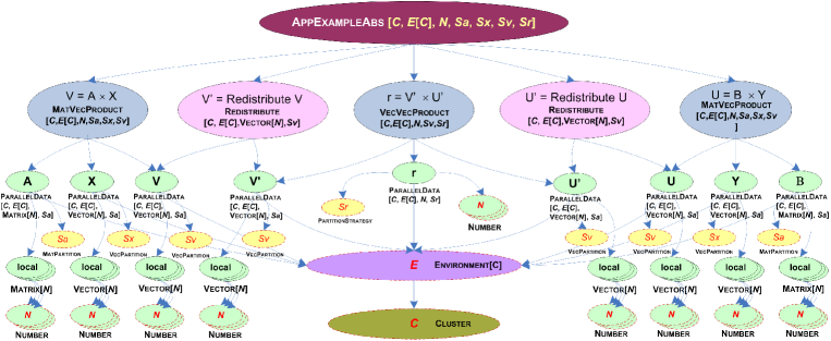
Figure 8: Hierarchy of Components of the Application Example

5 Implementation Issues

This section shows how the proposed type system has been implemented in HPE, the # programming system introduced in Section 2.2. The Back-End of HPE treats a #-component as a set of CLI/Mono object, each one associated to a unit, instantiated from a C# class. Therefore, the function $\mathcal{S}$ map configurations of abstract components to C# interfaces and configurations of #-components to C# classes that implement the interface associated to the configuration of the abstract component that it implements.

Let $C=\left[\makebox{\mbox{ \begin{minipage}{433.62pt} \par\begin{tabbing}\lx@intercol$\mathit{kind}\ C\ [X_{i}:T_{i}\ ^{i=1{\dots}n}]\ (a_{i}\ \ ^{i=1{\dots}k})$ \\ \hfil\lx@intercol\cr\lx@intercol$\mathbf{beg}$\=\hfil\lx@intercol&\lx@intercol$\mathbf{in}$ \\ \hfil\lx@intercol\cr\lx@intercol\>\hfil\lx@intercol&\lx@intercol$kind_{i}\ a_{i}:U_{i}\ (a_{r_{ij}}\ ^{j=1{\dots}p_{i}})\ \ ^{i=1{\dots}l}$\\ \hfil\lx@intercol\cr\lx@intercol\>\hfil\lx@intercol&\lx@intercol$\mathbf{unit}\ u_{i}\ \ \ ^{i=1{\dots}q}$ \\ \hfil\lx@intercol\cr\lx@intercol\>\hfil\lx@intercol&\lx@intercol$\mathbf{beg}$\=\hfil\lx@intercol&\lx@intercol$\mathbf{in}$ \\ \hfil\lx@intercol\cr\lx@intercol\>\hfil\lx@intercol&\lx@intercol\>\hfil\lx@intercol&\lx@intercol$\mathbf{slice}\ s_{ij}\ \mathbf{from}\ a_{z_{ij}}.v_{ij}\ \ ^{j=1{\dots}m_{i}}$ \\ \hfil\lx@intercol\cr\lx@intercol\>\hfil\lx@intercol&\lx@intercol\>\hfil\lx@intercol&\lx@intercol$\mathbf{action}\ A_{i}$\\ \hfil\lx@intercol\cr\lx@intercol\>\hfil\lx@intercol&\lx@intercol$\mathbf{end}$\\ \hfil\lx@intercol\cr\lx@intercol$\mathbf{end}$ \hfil\lx@intercol\end{tabbing}\par \end{minipage}} }\right]$ be a configuration schema of an abstract component. $\mathcal{S}(C)$ maps to a tuple of C# interfaces, one for each unit $u_{i}$, with the structure

namespace $C$
{
	public	interface $\mathbf{I}^{u_{i}}\left\langle\overline{\textbf{X}}\right\rangle:\mathbf{I}^{\mathit{kind}}$
		${\color[rgb]{0,0,1}\left[\makebox{\mbox{ \begin{minipage}{433.62pt} \par\begin{tabbing}\lx@intercol{\color[rgb]{0,0,0}where $X_{j}:\mathbf{I}^{T_{j}.w_{ij}}$} \hfil\lx@intercol\end{tabbing}\par \end{minipage}}}\ \ {\color[rgb]{1,0,0}\framebox{\rm a slice $T_{j}.w_{ij}$ exists (transitively) in $u_{i}$}}\ {\color[rgb]{0,1,0}\framebox{$X_{j}\in\overline{\textbf{X}}$}}\ \right]^{j=1\dots n}}$
	{
		${\color[rgb]{0,0,1}\left[\makebox{\mbox{ \begin{minipage}{433.62pt} \par\begin{tabbing}\lx@intercol{\color[rgb]{0,0,0}$\mathbf{I}^{U_{z_{ij}}.v_{ij}}$ $S_{ij}$ \{set;\};} \hfil\lx@intercol\end{tabbing}\par \end{minipage}}}\ \ {\color[rgb]{1,0,0}\framebox{$z_{ij}\in\{1,\dots,k\}$}}\ \right]^{j=1\dots m_{i}}}$
	}
}

The index $i$ refers to the unit ($u_{i}$). The interface declares a set of properties $S_{ij}$, one for each slice of the unit that corresponds to a unit of a public inner component. They require only their set access method. The reason will be clarified in the next paragraphs. The notation used for abstracting C# interface identifiers, $\mathbf{I}^{U_{z_{ij}}.v_{ij}}$, means the name of the C# interface that correspond to the unit $v_{ij}$ of the configuration $U_{z_{ij}}$.

Let $CImpl=\left[\makebox{\mbox{ \begin{minipage}{433.62pt} \par\begin{tabbing}\lx@intercol$\mathit{kind}\ $\=\hfil\lx@intercol&\lx@intercol$C\ [X_{i}:T_{i}\ \ ^{i=1{\dots}n}]$\\ \hfil\lx@intercol\cr\lx@intercol\>\hfil\lx@intercol&\lx@intercol$\mathbf{implements}\ C^{\prime}\ [X_{i}\ ^{i=1{\dots}n}]$ \\ \hfil\lx@intercol\cr\lx@intercol$\mathbf{beg}$\=\hfil\lx@intercol&\lx@intercol$\mathbf{in}$ \\ \hfil\lx@intercol\cr\lx@intercol\>\hfil\lx@intercol&\lx@intercol$\mathbf{unit}\ u_{i}\ \ \ ^{i=1{\dots}q}$ \\ \hfil\lx@intercol\cr\lx@intercol\>\hfil\lx@intercol&\lx@intercol$\mathbf{beg}$\=\hfil\lx@intercol&\lx@intercol$\mathbf{in}$ \\ \hfil\lx@intercol\cr\lx@intercol\>\hfil\lx@intercol&\lx@intercol\>\hfil\lx@intercol&\lx@intercol$\emph{{C}}_{i}$\\ \hfil\lx@intercol\cr\lx@intercol\>\hfil\lx@intercol&\lx@intercol$\mathbf{end}$\\ \hfil\lx@intercol\cr\lx@intercol$\mathbf{end}$ \hfil\lx@intercol\end{tabbing}\par \end{minipage}} }\right]$ be a configuration of a #-component. $\mathcal{S}(CImpl)$ maps to a set of C# classes, one for each unit $u_{i}$, with the following structure:

namespace $CImpl$
{
	public	class $\mathbf{H}^{u_{i}}\left\langle\overline{\textbf{X}}\right\rangle$: $\mathbf{Unit}$, $C.\mathbf{I}^{u_{i}}\left\langle\overline{\textbf{X}}\right\rangle$
		${\color[rgb]{0,0,1}\left[\makebox{\mbox{ \begin{minipage}{433.62pt} \par\begin{tabbing}\lx@intercol{\color[rgb]{0,0,0}where $X_{j}:\mathbf{I}^{T_{j}.w_{ij}}$} \hfil\lx@intercol\end{tabbing}\par \end{minipage}}}\ \ {\color[rgb]{1,0,0}\framebox{\rm a slice $T_{j}.w_{ij}$ exists (transitively) in $u_{i}$}}\ {\color[rgb]{0,1,0}\framebox{$X_{j}\in\overline{\textbf{X}}$}}\ \right]^{j=1\dots n_{i}}}$
	{
		// private slices
		${\color[rgb]{0,0,1}\left[\makebox{\mbox{{\color[rgb]{0,0,0} \begin{minipage}{433.62pt} \par\begin{tabbing}\lx@intercol private $\mathbf{I}^{U_{z_{ij}}.v_{ij}}$ $s_{ij}$ = null;\\ \hfil\lx@intercol\cr\lx@intercol private $\mathbf{I}^{U_{z_{ij}}.v_{ij}}$ $S_{ij}$ \\ \hfil\lx@intercol\cr\lx@intercol\{\=\hfil\lx@intercol&\lx@intercol\\ \hfil\lx@intercol\cr\lx@intercol\>\hfil\lx@intercol&\lx@intercol set \=\hfil\lx@intercol&\lx@intercol\{\ \=\hfil\lx@intercol&\lx@intercol\\ \hfil\lx@intercol\cr\lx@intercol\>\hfil\lx@intercol&\lx@intercol\>\hfil\lx@intercol&\lx@intercol\>\hfil\lx@intercol&\lx@intercol$s_{ij}=value$;\\ \hfil\lx@intercol\cr\lx@intercol\>\hfil\lx@intercol&\lx@intercol\>\hfil\lx@intercol&\lx@intercol\>\hfil\lx@intercol&\lx@intercol\hskip 22.76219pt \makebox{ \begin{math}{\color[rgb]{0,0,1}\left[\makebox{\mbox{ \begin{minipage}{433.62pt} \par\begin{tabbing}\lx@intercol{\color[rgb]{0,0,0}$s_{ik}.S^{\prime}_{i{jk}}=value$;} \hfil\lx@intercol\end{tabbing}\par \end{minipage}}}\ {\color[rgb]{1,0,0}\framebox{\rm$a_{z_{ik}}$ is a parameter of $a_{z_{ij}}$}}\ \right]^{k=1\dots m_{i}}}\end{math} }\\ \hfil\lx@intercol\cr\lx@intercol\>\hfil\lx@intercol&\lx@intercol\>\hfil\lx@intercol&\lx@intercol\} \\ \hfil\lx@intercol\cr\lx@intercol\} \hfil\lx@intercol\end{tabbing}\par \end{minipage}}}}\ {\color[rgb]{1,0,0}\framebox{$z_{ij}\in\{k{+}1,\dots,l\}$}}\ \right]^{j=1\dots m_{i}}}$
		// public slices
		${\color[rgb]{0,0,1}\left[\makebox{\mbox{{\color[rgb]{0,0,0} \begin{minipage}{433.62pt} \par\begin{tabbing}\lx@intercol private $\mathbf{I}^{U_{z_{ij}}.v_{ij}}$ $s_{ij}$ = null;\\ \hfil\lx@intercol\cr\lx@intercol public $\mathbf{I}^{U_{z_{ij}}.v_{ij}}$ $S_{ij}$ \\ \hfil\lx@intercol\cr\lx@intercol\{\=\hfil\lx@intercol&\lx@intercol\\ \hfil\lx@intercol\cr\lx@intercol\>\hfil\lx@intercol&\lx@intercol set \=\hfil\lx@intercol&\lx@intercol\{\ \=\hfil\lx@intercol&\lx@intercol\\ \hfil\lx@intercol\cr\lx@intercol\>\hfil\lx@intercol&\lx@intercol\>\hfil\lx@intercol&\lx@intercol\>\hfil\lx@intercol&\lx@intercol$s_{ij}=value$;\\ \hfil\lx@intercol\cr\lx@intercol\>\hfil\lx@intercol&\lx@intercol\>\hfil\lx@intercol&\lx@intercol\>\hfil\lx@intercol&\lx@intercol\hskip 22.76219pt \makebox{ \begin{math}{\color[rgb]{0,0,1}\left[\makebox{\mbox{ \begin{minipage}{433.62pt} \par\begin{tabbing}\lx@intercol{\color[rgb]{0,0,0}$s_{ik}.S^{\prime}_{i{jk}}=value$;} \hfil\lx@intercol\end{tabbing}\par \end{minipage}}}\ {\color[rgb]{1,0,0}\framebox{\rm$a_{z_{ik}}$ is a parameter of $a_{z_{ij}}$}}\ \right]^{k=1\dots m_{i}}}\end{math} }\\ \hfil\lx@intercol\cr\lx@intercol\>\hfil\lx@intercol&\lx@intercol\>\hfil\lx@intercol&\lx@intercol\} \\ \hfil\lx@intercol\cr\lx@intercol\} \hfil\lx@intercol\end{tabbing}\par \end{minipage}}}}\ {\color[rgb]{1,0,0}\framebox{$z_{ij}\in\{1,\dots,k\}$}}\ \right]^{j=1\dots m_{i}}}$
		// creation of private slices
		public void createSlices()
		{
			base.createSlices();
			${\color[rgb]{0,0,1}\left[\makebox{\mbox{ \begin{minipage}{433.62pt}\par\begin{tabbing}\lx@intercol{\color[rgb]{0,0,0}this.$S_{ij}$ = $\left(\mathbf{I}^{U_{z_{ij}}.v_{ij}}\right)$ \text@underline{BackEnd.createSlice}(this,$\dots$);} \hfil\lx@intercol\end{tabbing}\par\end{minipage}}}\ {\color[rgb]{1,0,0}\framebox{$z_{ij}\in\{k{+}1,\dots,l\}$}}\ \right]^{j=1\dots m_{i}}}$
		}
		$\emph{{C}}_{i}$ // kind dependent part
	}
}

The properties associated to the public slices of unit $u_{i}$, named $S_{ij}{{}^{\tiny\ |\ j\in\{1,\dots,m_{i}\}\wedge z_{ij}\in\{1,\dots,k\}}}$, required by interface $C.\mathbf{I}^{u_{i}}$, are implemented. In addition, there are private properties for the private slices of $u_{i}$, named $S_{ij}{{}^{\tiny\ |\ j\in\{1,\dots,m_{i}\}\wedge z_{ij}\in\{k{+}1,\dots,l\}}}$.

The public method createSlices and the static method BackEnd.createSlice form a mutually recursive pair. When creating a unit $u_{i}$ of a #-component $c$, createSlices calls BackEnd.createSlice to create the unit $v_{i{j}}$ of some private inner component $a_{z_{i{j}}}$ of $c$ that is a private slice $s_{i{j}}$ of $u_{i}$. Then, after instantiating $v_{i{j}}$, BackEnd.createSlice calls createSlices for creating its slices. The procedure proceeds recursively until units with no slices are reached (primitive units). In the return, the object that represents $v_{i{j}}$ is assigned to the slice property $S_{i{j}}$, causing a call of its writing access method (set). If $a_{z_{i{j}}}$ supplies any public inner component of another inner component $a_{z_{i{{k}}}}$, then $v_{ij}$ is also assigned to the corresponding public slice $S^{\prime}_{ijk}$ of $s_{i{{k}}}$, such that $s_{i{{k}}}{\mapsto}a_{z_{i{{k}}}}.v_{i{{k}}}\in\sigma_{i}$.

Moreover, BackEnd.createSlice is a parallel method, since $q$ simultaneous calls are performed to create a #-component $c$, each one executed by a process that has a unit $u_{i}\ ^{i=1{\dots}q}$ as slice. The $i^{th}$ call queries the DGAC (Distributed Global Assembly Cache), the HPE module responsible to manage parallel components, to find the class $\mathbf{H}^{u_{i}}$ that represent the unit $u_{i}$ of the best #-component, deployed in the environment, for the abstract component referred by the inner component in the configuration. For that, DGAC uses the resolution algorithm of Figure 7.

For each kind of #-component, it may be defined a dependent part, referred as $\emph{{C}}_{i}$ in the schema. More specifically, $\emph{{C}}_{i}$ is the implementation of the interface defined by the interface $\mathbf{I}^{\mathit{kind}}$. For example, for the kind computation, of HPE, it is defined the interface

inter	face IComputation {
	void compute();
}

,

whose method compute is implemented by the programmer to define the computation to be performed over the slices of each unit.

5.1 Case Study

Figure 8 depicts the hierarchy of components of a configuration of an abstract component of kind application for the parallel program of Section 2, named AppExampleAbs. The ellipses represent the transitive inner components that appear in the overall application. The arrows represent the “is inner component of” relation. The colors assigned to the abstract components distinguish their kinds. Dashed ellipses indicate parameters of the configuration, whose associated variable identifiers are italicized.

01. namespace example.computation.MatVecProduct 02. { 03. public interface ICalculate$<$C, E, N, Da, Dx, Dv$>$ 04 : IComputationKind 05. where C: ICluster 06. where E: IEnvironment$<$C$>$ 07. where N: INumber 08. where Da: IVecPartition 09. where Dx: IVecPartition 10. where Dv: IVecPartition 11. { 12. E Env {set;} 13. IParData$<$C, E, Matrix$<$N$>$, Da$>$ A {set;} 14. IParData$<$C, E, Vector$<$N$>$, Dx$>$ X {set;} 15. IParData$<$C, E, Vector$<$N$>$, Dv$>$ V {set;} 16. } 17. }

01. namespace example.computation.impl.MatVecProductImplForNumber { 02. public class HCalc ulate$<$C, E, N, Da, Dx, Dv$>$: Unit, ICalculate$<$C, E, D, Da, Dx, Dv$>$ 03. where C: IGNUCluster 04. where E: IMPIFull$<$C$>$ 05. where N: INumber 06. where Da: IByRows 07. where Dx: IReplicate 08. where Dv: IReplicate 09. { 10. private E env = null; 11. private IParData$<$C, E, Matrix$<$N$>$, Da$>$ a = null; 12. private IParData$<$C, E, Vector$<$N$>$, Dx$>$ x = null; 13. private IParData$<$C, E, Vector$<$N$>$, Dv$>$ v = null; 14. 15. public E Env { set { this.env = a.Env = x.Env = v.Env = value; } } 16. public IParData$<$C, E, Matrix$<$N$>$, Da$>$ A { set { this.a = value; } } 17. public IParData$<$C, E, Vector$<$N$>$, Dx$>$ X { set { this.x = value; } } 18. public IParData$<$C, E, Vector$<$N$>$, Dv$>$ V { set { this.v = value; } } 19. 20. public HCalculate() { $\cdots$ } 21. public void createSlices() { $\cdots$ } 22. public void compute() { 23. ($\cdots$) 24. IVector$<$N$>$ arr = V.Value; 25. ($\cdots$) 26. // 1st attempt (unsafe). line 33 causes type check error !!! 27. N newValue = new example.data.impl.NumberImpl.INumberImpl(); 28. ($\cdots$) 29. // 2nd attempt (safe). In line 36, using reflection, an instance of N is created. 30. N newValue = Activator.CreateInstance(typeof(N)); 31. ($\cdots$) 32. for (i=0; i¡=arr.size(); i++) arr.set(i, newValue); 33. ($\cdots$) 34. } 35. } 36. }

Figure 9: Unit of MatVecProduct and MatVecProductImplForNumber

The configuration of the inner component $\mathrm{V=A\times X}$ is MatVecProduct, discussed in Section 3. To illustrate how the proposed type system fits CTS (Common Type System), of CLI virtual machines, the interface ICalculate, associated with the units of the abstract component MatVecProduct, and the class HCalculate, associated with the units of MatVecProductImplForNumbers, are presented in Figure 9, obtained from the translation schemas introduced in the beginning of Section 5. MatVecProductImplForNumber differs from MatVecProductImplForDouble because it works with any number data type, including double precision float point ones.

It is important to understand how generic types of CLI are used to implement the relation between abstract components and their #-components. For instance, the interface ICalculate is generic in type variables $C$, $E$, $N$, $Sa$, $Sx$, and $Sv$, like MatVecProduct. HCalculate is also generic in the same type parameters, but their bounds are specialized for the types for which the class is tuned, making possible to make assumptions about the structure of objects of these types. In the method compute of HCalculate (lines 22 to 34), it is shown that CTS does not allow that one instantiates an object of class INumberImpl, implementing INumber, in a context where a object of type $N$, such that $N<:\texttt{INumber}$, is expected, like in line 27 (1st attempt). If the value of $N$ at run-time is a proper subtype of INumber, like IDouble, the assignment to array elements in line 32 is unsafe. On the other hand, if the variable newValue is instantiated like in line 30 (2nd attempt) it is created an object of the actual type of $N$, which can be IDouble safely. This is the reason why languages such as C# and Java only support invariant generic types ($T\langle{U}\rangle<:T^{\prime}\langle{U^{\prime}}\rangle\Leftrightarrow T<:T^{\prime}\wedge U=U^{\prime}$). In languages like Java, where generic types are implemented using type erasure, it is not possible to create an instance of the class associated to type variable $N$ at run-time, since type variables are erased in compilation. But this is possible in C#, using reflection, because the bytecode of CIL (Common Intermediate Language) carries generic types at runtime. This is one of the motivations to use Mono for implementing HPE.

6 Conclusions and Lines for Further Works

The # component model attempts to converge software engineering techniques and parallel programming artifacts, addressing the raising in complexity and scale of recent applications in HPC domains. The recent design and prototype of HPE, a # programming system, suggests gains in abstraction and modularity, without significant performance penalties. This paper introduced a type system for # programming systems that was applied to HPE, allowing the study of its formal properties, mainly regarding safety, compositionability, and expressiveness. It has been designed for allowing programmers to make assumptions about specific features of parallel computing architectures, but also providing the ability to work at some desired level of abstraction. This is possible due to a combination of existential and universal bounded quantification. In the near future, it is planned to research on the how other concepts found in higher-level type system designs may improve parallel programming practice.

References

- [Allan et al. 2002] Allan, B. A., Armstrong, R. C., Wolfe, A. P., Ray, J., Bernholdt, D. E., and Kohl, J. A. (2002). The CCA Core Specification in a Distributed Memory SPMD Framework. Concurrency and Computation: Practice and Experience, 14(5):323–345.
- [Alt et al. 2004] Alt, M., Dünnweber, J., Müller, J., and Gorlatch, S. (2004). HOCs: Higher-Order Components for Grids. In Workshop on Component Models and Systems for Grid Applications (in ICS’2004). Kluwer Academics.
- [Armstrong et al. 2006] Armstrong, R., Kumfert, G., McInnes, L. C., Parker, S., Allan, B., Sottile, M., Epperly, T., and Dahlgreen Tamara (2006). The CCA Component Model For High-Performance Scientific Computing. Concurrency and Computation: Practice and Experience, 18(2):215–229.
- [Baduel et al. 2007] Baduel, L., Baude, F., and Caromel, D. (2007). Asynchronous Typed Object Groups for Grid Programming. Journal of Parallel Programming, 35(6):573–613.
- [Baude et al. 2007] Baude, F., Caromel, D., Henrio, L., and Morel, M. (2007). Collective Interfaces for Distributed Components. In 7th International Symposium on Cluster Computing and the Grid (CCGrid 07). IEEE Computer Society.
- [Baude et al. 2008] Baude, F., Caromel, F., Dalmasso, C., Danelutto, M., Getov, W., Henrio, L., and Pérez, C. (2008). GCM: A Grid Extension to Fractal for Autonomous Distributed Components. Annals of Telecommunications, 0:000–000.
- [Bernholdt D. E. et al. 2004] Bernholdt D. E., Nieplocha, J., and Sadayappan, P. (2004). Raising Level of Programming Abstraction in Scalable Programming Models. In IEEE International Conference on High Performance Computer Architecture (HPCA), Workshop on Productivity and Performance in High-End Computing (P-PHEC), pages 76–84. Madrid, Spain, IEEE Computer Society.
- [Bruneton et al. 2002] Bruneton, E., Coupaye, T., and Stefani, J. B. (2002). Recursive and Dynamic Software Composition with Sharing. In European Conference on Object Oriented Programming (ECOOP’2002). Springer.
- [Carvalho Junior et al. 2007] Carvalho Junior, F. H., Lins, R., Correa, R. C., and Araújo, G. A. (2007). Towards an Architecture for Component-Oriented Parallel Programming. Concurrency and Computation: Practice and Experience, 19(5):697–719. Special Issue: Component and Framework Technology in High-Performance and Scientific Computing. Edited by David E. Bernholdt.
- [Carvalho Junior and Lins 2008] Carvalho Junior, F. H. and Lins, R. D. (2008). An Institutional Theory for #-Components. Electronic Notes in Theoretical Computer Science, 195:113–132.
- [Carvalho Junior and Lins 2009] Carvalho Junior, F. H. and Lins, R. D. (2009). Compositional Specification of Parallel Programs Using Circus. Electronic Notes in Theoretical Computer Science, 0000:0–0. 5th International Workshop on Formal Aspects of Component Software.
- [Dongarra et al. 1996] Dongarra, J., Otto, S. W., Snir, M., and Walker, D. (1996). A Message Passing Standard for MPP and Workstation. Communications of ACM, 39(7):84–90.
- [Milli et al. 2004] Milli, H., Elkharraz, A., and Mcheick, H. (2004). Understanding Separation of Concerns. In Workshop on Early Aspects - Aspect Oriented Software Development (AOSD’04), pages 411–428.
- [Pierce 2002] Pierce, B. (2002). Types and Programming Languages. The MIT Press.
- [Post and Votta 2005] Post, D. E. and Votta, L. G. (2005). Computational Science Demands a New Paradigm. Physics Today, 58(1):35–41.
- [Sarkar et al. 2004] Sarkar, V., Williams, C., and Ebciolu, K. (2004). Application Development Productivity Challenges for High-End Computing. In IEEE International Conference on High Performance Computer Architecture (HPCA), Workshop on Productivity and Performance in High-End Computing, pages 14–18.
- [van der Steen 2006] van der Steen, A. J. (2006). Issues in Computational Frameworks. Concurrency and Computation: Practice and Experience, 18(2):141–150.
- [Wang and Qian 2005] Wang, A. J. A. and Qian, K. (2005). Component-Oriented Programming. Wiley-Interscience.