1/R Correction to Gravity in the Early Universe

Abstract

To explain the accelerated expansion of the late universe, the $1/R$ correction to Einstein gravity is usually considered, where $R$ is the Ricci scalar. This correction term, if stable, is generally believed to be negligible during inflation. However, if the $1/R$ term is inflaton-dependent, it will dramatically change the story of inflation. The entropy perturbation will naturally appear and drive the evolution of curvature perturbation outside the Hubble horizon. In a large class of models, the entropy perturbation can be made nearly scale-invariant. In Einstein gravity the single-field inflation with a quartic potential has been ruled out by recent observations, but it revives when the $1/R$ term is turned on. The evolution of non-Gaussianities on large scale are also studied and applied to inflation with $1/R$ correction. In some specific models, a large non-Gaussianity can be naturally generated outside the horizon. Recent study ruled out almost all $f(R)$ models during matter dominated phase. Taking this into consideration, we are left with a limited class of model which recovers the Einstein gravity soon after reheating.

I Introduction

Despite great achievements of Einstein’s gravity theory, numerous versions of its modification or extension have been proposed in the last and this century. Some proposals came and went, while others were tightly constrained by observations Turyshev:2008ur . One of the modern motivations for modifying Einstein gravity is attempting to explain the accelerated expansion of the late universe Riess:1998cb ; Perlmutter:1998np ; Komatsu:2008hk . Rather than introducing a cosmological constant or an unknown dark energy, one can explain the cosmic acceleration by designing a modified theory of gravity, see typical models in Dvali:2000hr ; Carroll:2003wy ; Li:2004rb for instance. Among the nonlinear modifications Nojiri:2006ri ; Sotiriou:2008rp , namely $f(R)$ gravity theories, the most disputed one is a model with $1/R$ correction to the Einstein action Carroll:2003wy ,

$$S=\frac{M_{p}^{2}}{2}\int d^{4}x\sqrt{-g}\left(R-\frac{\mu^{4}}{R}\right)+\int d^{4}x\sqrt{-g}\mathcal{L}_{M},$$ (1)

though such a term looks bizarre from the viewpoint of effective field theory.

In reference Carroll:2003wy , it was assumed that the $1/R$ term was negligibly small in the early universe but gradually reveals itself as the universe becomes more and more flat (the Ricci scalar $R$ gets smaller and smaller) at the late time. However, in general the parameter $\mu$ may depend on some matter fields and therefore evolve along with the matter fields. Indeed, the general coupling between gravity and the matter sector was considered in recent investigations Amendola:2006kh ; Amendola:2006eh ; Song:2006ej ; Sawicki:2007tf ; Nesseris:2008mq ; Sadeghi:2009qr ; Bertolami:2009cd ; Ito:2009nk . Especially, the parameter $\mu$ can be a function of the inflaton field, which will induce a correction term to single-field inflation,

$$S=\int d^{4}x\sqrt{-g}\left[\frac{1}{2}M_{p}^{2}R+\frac{g(\varphi)}{2R}-\frac{1}{2}g^{\alpha\beta}\partial_{\alpha}\varphi\partial_{\beta}\varphi-V(\varphi)\right].$$ (2)

We expect the correction term was not negligible during inflation but decayed soon after inflation (during reheating). By fine-tuning the coupling $g(\varphi)$, one may also expect action (2) reproduces (1) in the late universe. Please refer to Liddle:2008bm for a delicate model unifying inflaton, dark matter and dark energy with a single field.

In fact, the action (2) is just a special case of the $f(\varphi,R)$ generalized gravity, see Ji:2009yw ; Hwang:1990re ; Hwang:1996np ; Hwang:1996bc ; Hwang:1997uc ; Hwang:2005hb ; Chen:2006wn and references therein. So we can employ the formalism recently developed in Ji:2009yw to deal with this model. In section II we will collect the main results of Ji:2009yw , in a way as general as possible. The non-Gaussianity in $f(\varphi,R)$ theory has not been studied previously and deserves a separate investigation. But a semi-quantitative analysis of this problem will be presented in section III. Then these formulas will be applied to model (2) in section IV, where we also find out the conditions for generating nearly scale-invariant power spectra. Based on these results, we will in sections V and VI study models with specific potentials, i.e., $V(\varphi)=\frac{1}{2}m^{2}\varphi^{2}$ and $V(\varphi)=\lambda\varphi^{4}$ respectively. The five-year Wilkinson Microwave Anisotropy Probe (WMAP5) has ruled out single-field inflation with $V(\varphi)=\lambda\varphi^{4}$ in Einstein gravity, because in this model the tensor-to-scalar ratio $r_{T}$ is too large and the the power spectrum of curvature perturbation $P_{\mathcal{R}}$ is over-tilted Komatsu:2008hk . Interestingly, our results will show that, in $V(\varphi)=\lambda\varphi^{4}$ model, $r_{T}$ can be depressed by an order of magnitude while $P_{\mathcal{R}}$ can be less tiled due to the $1/R$ term, hence the model can pass the WMAP5 test. In the past few years, by considering the coupling to matter in high redshift Amendola:2006kh ; Amendola:2006eh , it was found that there are instabilities in some branches of $f(R)$ gravity models Song:2006ej ; Sawicki:2007tf . Therefore, in section VII, we analyze the stability problem for our models and its implication to post-inflation evolutions. We will conclude in the last section after a few remarks on the possible loopholes and the resulting uncertainty of our calculations. In appendix A we will derive some useful formulas for three-point correlation functions of entropy and curvature perturbations. The formulas developed in section III and appendix A are very general and can be applied to other inflation models with weakly coupled multiple fields.

II Inflation in Generalized Gravity

There has been a lot of investigations on perturbation theory in generalized gravity, where the Ricci scalar and a scalar field are non-minimally coupled via an arbitrary function Hwang:1990re ; Hwang:1996np ; Hwang:1996bc ; Hwang:1997uc ; Hwang:2005hb ; Chen:2006wn :

$$S=\int d^{4}x\sqrt{-g}\left[\frac{1}{2}f(\varphi,R)-\frac{1}{2}g^{\alpha\beta}\partial_{\alpha}\varphi\partial_{\beta}\varphi-V(\varphi)\right].$$ (3)

But most of them are restricted to special cases with only one degree of freedom, although it was believed that there should be two degrees of freedom in general Teyssandier:1983zz ; Maeda:1988ab ; Wands:1993uu . In a recent research Ji:2009yw , such an $f(\varphi,R)$ theory was reanalyzed by incorporating the other degree of freedom and the entropy perturbation. Being interested in its implication to inflation, here we will gather the general relevant results. In an independent work Matsuda:2009np , starting with more general kinetic terms and more scalar fields, the evolution of the “perturbed expansion rate” was calculated for generalized gravity theory using the techniques invented by Wands:2000dp . We will mainly follow the conventions and notations in Ji:2009yw . For instance, the signature of metric is $(-+++)$, and we will take

$$M_{p}^{-2}=8\pi G,\leavevmode\nobreak\ \leavevmode\nobreak\ \leavevmode\nobreak\ \leavevmode\nobreak\ R=6(2H^{2}+\dot{H}),\leavevmode\nobreak\ \leavevmode\nobreak\ \leavevmode\nobreak\ \leavevmode\nobreak\ F=\frac{\partial}{\partial R}f(\varphi,R),\leavevmode\nobreak\ \leavevmode\nobreak\ \leavevmode\nobreak\ \leavevmode\nobreak\ E=\frac{2HF+\dot{F}}{F^{\frac{3}{2}}}.$$ (4)

All of the general results have appeared in Ji:2009yw , partly mixing with some special models. Nevertheless, it is still helpful to put them orderly in this section.

First of all, let us define the slow-roll parameters:

$$\epsilon_{1}=\frac{\dot{H}}{H^{2}},\leavevmode\nobreak\ \leavevmode\nobreak\ \leavevmode\nobreak\ \leavevmode\nobreak\ \epsilon_{2}=\frac{\ddot{H}}{H\dot{H}},\leavevmode\nobreak\ \leavevmode\nobreak\ \leavevmode\nobreak\ \leavevmode\nobreak\ \eta_{1}=\frac{\ddot{\varphi}}{H\dot{\varphi}},$$

$$\eta_{2}=\frac{\dddot{\varphi}}{H\ddot{\varphi}},\leavevmode\nobreak\ \leavevmode\nobreak\ \leavevmode\nobreak\ \leavevmode\nobreak\ \delta_{1}=\frac{\dot{F}}{HF},\leavevmode\nobreak\ \leavevmode\nobreak\ \leavevmode\nobreak\ \leavevmode\nobreak\ \delta_{2}=\frac{\dot{E}}{HE},$$

$$\delta_{3}=\frac{\ddot{F}}{H\dot{F}},\leavevmode\nobreak\ \leavevmode\nobreak\ \leavevmode\nobreak\ \leavevmode\nobreak\ \delta_{4}=\frac{\ddot{E}}{H\dot{E}},\leavevmode\nobreak\ \leavevmode\nobreak\ \leavevmode\nobreak\ \leavevmode\nobreak\ \delta_{6}=\frac{\dddot{E}}{H\ddot{E}}\leavevmode\nobreak\ .$$ (5)

Be careful with the notation and sign difference between the slow-roll parameters here and those in most literature. The slow-roll conditions are met if the absolute values of these parameters are much smaller than unity. Under the slow-roll conditions, the background equations can be approximately written as

$$V-\frac{1}{2}f+3H^{2}F\simeq 0,$$

$$\dot{\varphi}^{2}+2\dot{H}F-H\dot{F}\simeq 0,$$

$$3H\dot{\varphi}-\frac{1}{2}f_{,\varphi}+V_{,\varphi}\simeq 0.$$ (6)

These equations and the slow-roll conditions also result in the following useful relations

$$\dot{E}=-\frac{\dot{\varphi}^{2}}{F^{\frac{3}{2}}},\leavevmode\nobreak\ \leavevmode\nobreak\ \leavevmode\nobreak\ \leavevmode\nobreak\ \ddot{E}=\frac{3\dot{F}\dot{\varphi}^{2}-4F\dot{\varphi}\ddot{\varphi}}{2F^{\frac{5}{2}}},\leavevmode\nobreak\ \leavevmode\nobreak\ \leavevmode\nobreak\ \leavevmode\nobreak\ \delta_{2}\simeq\epsilon_{1}-\frac{1}{2}\delta_{1},$$

$$\delta_{4}\simeq 2\eta_{1}-\frac{3}{2}\delta_{1},\leavevmode\nobreak\ \leavevmode\nobreak\ \leavevmode\nobreak\ \leavevmode\nobreak\ \delta_{6}\simeq\eta_{1}-\frac{5}{2}\delta_{1}+\frac{3\delta_{1}\delta_{3}-\delta_{1}\eta_{1}-4\eta_{1}\eta_{2}}{3\delta_{1}-4\eta_{1}}.$$ (7)

In the longitudinal gauge, the Friedmann-Lemaître-Robertson-Walker (FLRW) metric with scalar type perturbations is given by

$$ds^{2}=-(1+2\phi)dt^{2}+a^{2}(1-2\psi)\delta_{ij}dx^{i}dx^{j}.$$ (8)

For generalized gravity, usually $\phi\neq\psi$, so we will have two degrees of freedom after eliminating the inflaton fluctuation $\delta\varphi$. The perturbed Einstein equations will give us two coupled second-order differential equations for ($\phi$, $\psi$). So we say there are two dynamical degrees of freedom. But this pair of variables can be traded for ($\mathcal{R}$, $\mathcal{S}$) or ($v_{\mathcal{R}}$, $v_{\mathcal{S}}$) or ($u_{\mathcal{R}}$, $u_{\mathcal{S}}$) by the following relations:

$$\mathcal{R} = \frac{1}{2}(\phi+\psi)+\frac{2HF+\dot{F}}{2F\dot{\varphi}^{2}+3\dot{F}^{2}}\left[F(\dot{\phi}+\dot{\psi})+\frac{1}{2}(2HF+\dot{F})(\phi+\psi)\right],$$

$$\mathcal{S} = \frac{\dot{F}}{\dot{\varphi}}\sqrt{\frac{3}{2F}}\left[\frac{F(2HF+\dot{F})}{2F\dot{\varphi}^{2}+3\dot{F}^{2}}(\dot{\phi}+\dot{\psi})+\frac{(2HF+\dot{F})^{2}}{4F\dot{\varphi}^{2}+6\dot{F}^{2}}(\phi+\psi)+\frac{2HF+\dot{F}}{2\dot{F}}(\phi-\psi)\right],$$

$$v_{\mathcal{R}} = \frac{a\sqrt{2F(2F\dot{\varphi}^{2}+3\dot{F}^{2})}}{2HF+\dot{F}}\mathcal{R},\leavevmode\nobreak\ \leavevmode\nobreak\ \leavevmode\nobreak\ \leavevmode\nobreak\ v_{\mathcal{S}}=\frac{a\sqrt{2F(2F\dot{\varphi}^{2}+3\dot{F}^{2})}}{2HF+\dot{F}}\mathcal{S},$$

$$u_{\mathcal{R}} = \frac{F^{\frac{3}{2}}}{\sqrt{4F\dot{\varphi}^{2}+6\dot{F}^{2}}}(\phi+\psi),\leavevmode\nobreak\ \leavevmode\nobreak\ \leavevmode\nobreak\ \leavevmode\nobreak\ u_{\mathcal{S}}=\frac{a\sqrt{F(2F\dot{\varphi}^{2}+3\dot{F}^{2})}}{\sqrt{3}(2HF+\dot{F})}\mathcal{S}.$$ (9)

We have chosen the normalization for $\mathcal{S}$ so that $\mathcal{P}_{\mathcal{R}\ast}=\mathcal{P}_{\mathcal{S}\ast}$ when perturbations cross the Hubble horizon, as will be given by equation (II). In reference Ji:2009yw , $\mathcal{R}$ is interpreted as the curvature perturbation while $\mathcal{S}$ is interpreted as the entropy perturbation. $v_{\mathcal{R}}$ and $v_{\mathcal{S}}$ are the corresponding canonical variables. The interpretation of $u_{\mathcal{R}}$ and $u_{\mathcal{S}}$ is less clear, but are defined for our convenience, and one may think $u_{\mathcal{R}}$ as as something akin to the canonical momenta (not exactly). In terms of them, the evolution equations of perturbations take the form

$$u^{\prime\prime}_{\mathcal{R}k}+k^{2}u_{\mathcal{R}k}+m_{\mathcal{R}}^{2}a^{2}u_{\mathcal{R}k}+\beta u_{\mathcal{S}k} = 0,$$

$$u^{\prime\prime}_{\mathcal{S}k}+k^{2}u_{\mathcal{S}k}+m_{\mathcal{S}}^{2}a^{2}u_{\mathcal{S}k}+\alpha k^{2}u_{\mathcal{R}k} = 0,$$ (10)

whose coefficients

$$\frac{m_{\mathcal{R}}^{2}}{H^{2}}\simeq 2\epsilon_{1}-\eta_{1},\leavevmode\nobreak\ \leavevmode\nobreak\ \leavevmode\nobreak\ \leavevmode\nobreak\ \beta\simeq\mbox{sign}(\dot{\varphi})aH\sqrt{\delta_{1}-2\epsilon_{1}},$$

$$\alpha\simeq\mbox{sign}(\dot{\varphi})\frac{2}{3}aH\sqrt{\delta_{1}-2\epsilon_{1}},$$

$$\frac{m_{\mathcal{S}}^{2}}{H^{2}}\simeq\frac{5}{2}\delta_{1}-5\epsilon_{1}+\frac{F}{3H^{2}F_{,R}}+\frac{\dot{F}F_{,\varphi}}{2H^{2}F_{,R}\dot{\varphi}}-6.$$ (11)

As is well known, couple is trouble. This also applies to the coupled equations (II). To make our analysis simple, for perturbations inside the Hubble horizon, we will always disregard the coupling terms controlled by $\beta$ and $\alpha$ (decoupled approximation). This enables us to get a rough estimation but also induces some uncertainties. Imposing an appropriate quantized initial condition at $k\gg aH$, we find an analytical solution under the decoupled approximation,

$$u_{\mathcal{R}k}=-\frac{1}{4k^{\frac{3}{2}}}e^{i(\nu_{1}-\frac{1}{2})\frac{\pi}{2}}\sqrt{-\pi k\tau}H^{(1)}_{\nu_{1}}(-k\tau)\hat{e}_{\mathcal{R}k}, \text{with}\leavevmode\nobreak\ \nu_{1}^{2}=\frac{1}{4}-\frac{m_{\mathcal{R}}^{2}}{H^{2}},$$

$$u_{\mathcal{S}k}=-\frac{1}{2\sqrt{6k}}e^{i(\nu_{2}-\frac{3}{2})\frac{\pi}{2}}\sqrt{-\pi k\tau}H^{(1)}_{\nu_{2}}(-k\tau)\hat{e}_{\mathcal{S}k}, \text{with}\leavevmode\nobreak\ \nu_{2}^{2}=\frac{1}{4}-\frac{m_{\mathcal{S}}^{2}}{H^{2}}.$$ (12)

Here $\{\hat{e}_{\mathcal{R}k},\hat{e}_{\mathcal{S}k}\}$ is the orthonormal basis

$$\langle\hat{e}_{\alpha k},\hat{e}_{\beta k^{\prime}}\rangle=\delta_{\alpha\beta}\delta(k-k^{\prime}),\leavevmode\nobreak\ \leavevmode\nobreak\ \leavevmode\nobreak\ \leavevmode\nobreak\ \alpha,\beta=\mathcal{R},\mathcal{S}.$$ (13)

The normalization of Fourier modes $\mathcal{R}_{k}$ and $\mathcal{S}_{k}$ is exhibited by equation (70) in appendix A. If $m_{\mathcal{R}}^{2}/H^{2}\simeq 0$ and $m_{\mathcal{S}}^{2}/H^{2}\simeq-2$, then the power spectra at the horizon-crossing $k=aH$ are nearly scale-invariant,

$$\mathcal{P}_{\mathcal{R}\ast} = \frac{k^{3}}{2\pi^{2}}|\mathcal{R}_{k\ast}|^{2}\simeq\left.\frac{H^{4}}{4\pi^{2}\dot{\varphi}^{2}}\right|_{\ast},$$

$$\mathcal{P}_{\mathcal{S}\ast} = \frac{k^{3}}{2\pi^{2}}|\mathcal{S}_{k\ast}|^{2}\simeq\left.\frac{H^{4}}{4\pi^{2}\dot{\varphi}^{2}}\right|_{\ast}.$$ (14)

The condition $m_{\mathcal{R}}^{2}/H^{2}\simeq 0$ is trivial due to the slow-roll conditions. But $m_{\mathcal{S}}^{2}/H^{2}\simeq-2$ puts a nontrivial constraint on viable models. Throughout this paper, an asterisk means the quantities take their horizon-crossing value. Since we have neglected the coupling between curvature perturbation and entropy perturbation inside the horizon, their cross-correlation is negligible at the Hubble-crossing,

$$\mathcal{P}_{\mathcal{C}\ast}=\frac{k^{3}}{2\pi^{2}}\langle\mathcal{R}_{k\ast},\mathcal{S}_{k\ast}\rangle\simeq 0.$$ (15)

When crossing the horizon, the spectral indices are

$$n_{\mathcal{R}\ast}-1=n_{\mathcal{S}\ast}-1=4\epsilon_{1\ast}-2\eta_{1\ast}.$$ (16)

Unlike the single-field inflation in Einstein gravity, the entropy perturbation and curvature perturbation are not conserved even well outside the horizon $k\ll aH$. It is more convenient to follow their evolution in terms of ($\mathcal{R}$, $\mathcal{S}$). If $m_{\mathcal{S}}^{2}/H^{2}\simeq-2$, we have $\ddot{\mathcal{S}}_{k}/(H\dot{\mathcal{S}}_{k})\sim\mathcal{O}(\epsilon)$ and hence

$$\dot{\mathcal{S}}_{k}=\mu_{\mathcal{S}}H\mathcal{S}_{k}, \mu_{\mathcal{S}}=-\frac{1}{3}\left(\frac{m_{\mathcal{S}}^{2}}{H^{2}}+2+\epsilon_{1}-\frac{9}{4}\delta_{1}-3\delta_{2}+\frac{3}{2}\delta_{4}\right),$$

$$\dot{\mathcal{R}}_{k}=\mu_{\mathcal{R}}H\mathcal{S}_{k}, \mu_{\mathcal{R}}=\frac{\mbox{sign}(\dot{\varphi})}{\delta_{1}}\sqrt{\frac{2(\delta_{1}-2\epsilon_{1})}{3}}\left(2\eta_{1}-\frac{5}{2}\delta_{1}-\delta_{4}\right).$$ (17)

Taking $\mu_{\mathcal{S}}$ and $\mu_{\mathcal{R}}$ as constants approximately, its analytical solution reads

$$\mathcal{S}_{k}=\mathcal{S}_{k\ast}\exp\left(\int_{t_{\ast}}^{t}\mu_{\mathcal{S}}Hdt\right)=\mathcal{S}_{k\ast}e^{\mu_{\mathcal{S}}(N_{\ast}-N)},$$

$$\mathcal{R}_{k}-\mathcal{R}_{k\ast}=\int_{t_{\ast}}^{t}\mu_{\mathcal{R}}H\mathcal{S}_{k}dt=\frac{\mu_{\mathcal{R}}}{\mu_{\mathcal{S}}}\mathcal{S}_{k\ast}\left[e^{\mu_{\mathcal{S}}(N_{\ast}-N)}-1\right],$$ (18)

in which $N=\ln[a_{end}/a(t)]$ stands for the e-folding number from time $t$ to the end of inflation.

As a result, on the super-hubble scale, the power spectra are

$$\mathcal{P}_{\mathcal{R}}\simeq\mathcal{P}_{\mathcal{R}\ast}+\mathcal{P}_{\mathcal{S}\ast}\frac{\mu_{\mathcal{R}}^{2}}{\mu_{\mathcal{S}}^{2}}\left[e^{\mu_{\mathcal{S}}(N_{\ast}-N)}-1\right]^{2},$$

$$\mathcal{P}_{\mathcal{S}}\simeq\mathcal{P}_{\mathcal{S}\ast}e^{2\mu_{\mathcal{S}}(N_{\ast}-N)},$$

$$\mathcal{P}_{\mathcal{C}}\simeq\mathcal{P}_{\mathcal{S}\ast}\frac{\mu_{\mathcal{R}}}{\mu_{\mathcal{S}}}e^{\mu_{\mathcal{S}}(N_{\ast}-N)}\left[e^{\mu_{\mathcal{S}}(N_{\ast}-N)}-1\right].$$ (19)

Their spectral indices are

$$n_{\mathcal{R}}-1 = n_{\mathcal{S}\ast}-1-\frac{2\mu_{\mathcal{R}}^{2}\mu_{\mathcal{S}}e^{\mu_{\mathcal{S}}(N_{\ast}-N)}\left[e^{\mu_{\mathcal{S}}(N_{\ast}-N)}-1\right]}{\mu_{\mathcal{S}}^{2}+\mu_{\mathcal{R}}^{2}\left[e^{\mu_{\mathcal{S}}(N_{\ast}-N)}-1\right]^{2}},$$

$$n_{\mathcal{S}}-1 = n_{\mathcal{S}\ast}-1-2\mu_{\mathcal{S}},$$

$$n_{\mathcal{C}}-1 = n_{\mathcal{S}\ast}-1-\frac{\mu_{\mathcal{S}}\left[2e^{\mu_{\mathcal{S}}(N_{\ast}-N)}-1\right]}{e^{\mu_{\mathcal{S}}(N_{\ast}-N)}-1}.$$ (20)

We have defined the entropy-to-curvature ratio in Ji:2009yw

$$r_{\mathcal{S}}=\frac{\mathcal{P}_{\mathcal{S}}}{\mathcal{P}_{\mathcal{R}}}.$$ (21)

The tensor type perturbation is conserved outside the horizon. Its power spectrum is relatively simple Hwang:2005hb

$$\mathcal{P}_{T}\simeq\frac{2H^{2}}{\pi^{2}F}=\mathcal{P}_{\mathcal{S}\ast}(8\delta_{1}-16\epsilon_{1}),$$ (22)

with a spectral index

$$n_{T}\simeq\frac{2\dot{H}}{H^{2}}-\frac{\dot{F}}{HF}=2\epsilon_{1}-\delta_{1}.$$ (23)

Here we have used a normalization different from Hwang:2005hb ; Ji:2009yw to accommodate to the WMAP5 convention Komatsu:2008hk .

The above results hold generally for slow-roll inflation in generalized $f(\varphi,R)$ gravity with $F>0$, as long as the entropy perturbation is non-vanishing and nearly scale-invariant. For details of derivation and explanations, one can refer to Ji:2009yw .

It proves helpful to utilize also the entropy-curvature correlation angle $\Delta$ Wands:2002bn and the tensor-to-scalar ratio $r_{T}$

$$\cos\Delta=\frac{\mathcal{P}_{\mathcal{C}}}{\sqrt{\mathcal{P}_{\mathcal{R}}\mathcal{P}_{\mathcal{S}}}},\leavevmode\nobreak\ \leavevmode\nobreak\ \leavevmode\nobreak\ \leavevmode\nobreak\ r_{T}=\frac{\mathcal{P}_{T}}{\mathcal{P}_{\mathcal{R}}},$$ (24)

as well as a general transfer matrix

$$\left(\begin{array}[]{c}\mathcal{R}\\ \mathcal{S}\end{array}\right)=\left(\begin{array}[]{cc}1&T_{\mathcal{R}\mathcal{S}}\\ 0&T_{\mathcal{S}\mathcal{S}}\end{array}\right)\left(\begin{array}[]{c}\mathcal{R}\\ \mathcal{S}\end{array}\right)_{\ast}.$$ (25)

In fact, $\cos\Delta$ is nothing else but the correlation coefficient introduced in Langlois:1999dw .

III Non-Gaussianity

The primordial non-Gaussianity has attracted a lot of attention during recent years. To judge whether we can get some interesting large non-Gaussianity before expanding actions to the third order and calculating the three-point correlation functions, we can make some semi-quantitative estimates using the results of single-field inflation in Einstein gravity theory.

We start with the calculation of three-point correlation of curvature perturbations $\mathcal{R}$, by virtue of (25),

$$\langle\mathcal{R}(\mathbf{k}_{1})\mathcal{R}(\mathbf{k}_{2})\mathcal{R}(\mathbf{k}_{3})\rangle$$ (26)

$$= \langle(\mathcal{R}(\mathbf{k}_{1})_{\ast}+T_{\mathcal{RS}}\mathcal{S}(\mathbf{k}_{1})_{\ast})(\mathcal{R}(\mathbf{k}_{2})_{\ast}+T_{\mathcal{RS}}\mathcal{S}(\mathbf{k}_{2})_{\ast})(\mathcal{R}(\mathbf{k}_{3})_{\ast}+T_{\mathcal{RS}}\mathcal{S}(\mathbf{k}_{3})_{\ast})\rangle$$

$$= \langle\mathcal{S}(\mathbf{k}_{1})_{\ast}\mathcal{S}(\mathbf{k}_{2})_{\ast}\mathcal{S}(\mathbf{k}_{3})_{\ast}\rangle T_{\mathcal{RS}}^{3}$$

$$+\left[\langle\mathcal{R}(\mathbf{k}_{3})_{\ast}\mathcal{S}(\mathbf{k}_{1})_{\ast}\mathcal{S}(\mathbf{k}_{2})_{\ast}\rangle+\langle\mathcal{R}(\mathbf{k}_{2})_{\ast}\mathcal{S}(\mathbf{k}_{3})_{\ast}\mathcal{S}(\mathbf{k}_{1})_{\ast}\rangle+\langle\mathcal{R}(\mathbf{k}_{1})_{\ast}\mathcal{S}(\mathbf{k}_{2})_{\ast}\mathcal{S}(\mathbf{k}_{3})_{\ast}\rangle\right]T_{\mathcal{RS}}^{2}$$

$$+\left[\langle\mathcal{R}(\mathbf{k}_{2})_{\ast}\mathcal{R}(\mathbf{k}_{3})_{\ast}\mathcal{S}(\mathbf{k}_{1})_{\ast}\rangle+\langle\mathcal{R}(\mathbf{k}_{1})_{\ast}\mathcal{R}(\mathbf{k}_{3})_{\ast}\mathcal{S}(\mathbf{k}_{2})_{\ast}\rangle+\langle\mathcal{R}(\mathbf{k}_{1})_{\ast}\mathcal{R}(\mathbf{k}_{2})_{\ast}\mathcal{S}(\mathbf{k}_{3})_{\ast}\rangle\right]T_{\mathcal{RS}}$$

$$+\langle\mathcal{R}(\mathbf{k}_{1})_{\ast}\mathcal{R}(\mathbf{k}_{2})_{\ast}\mathcal{R}(\mathbf{k}_{3})_{\ast}\rangle,$$

where an asterisk means the quantities are calculated at the time of horizon-crossing $k=aH$. In the above equation, we assumed the linear evolution of $\mathcal{R}_{k}$ and $\mathcal{S}_{k}$ outside the horizon. Although this assumption is good enough for our semi-quantitative analysis, in a more accurate treatment, one should consider the nonlinear effects. There are two sources of nonlinear effects outside the horizon: the $\ddot{S}_{k}$ term neglected in equation (II); the time dependence of $\mu_{\mathcal{S}}$ and $\mu_{\mathcal{R}}$.

As we have mentioned, the curvature perturbation and the entropy perturbation are coupled. But, under our approximation, their coupling inside the horizon will not be taken into consideration in the estimation of magnitude. Because all of these quantities are calculated at horizon-crossing, we can treat the adiabatic and entropy perturbations independently. Using the single-field relations Komatsu:2001rj ; Chen:2006nt ,

$$\langle\mathcal{R}(\mathbf{k}_{1})_{\ast}\mathcal{R}(\mathbf{k}_{2})_{\ast}\mathcal{R}(\mathbf{k}_{3})_{\ast}\rangle = (2\pi)^{5/2}\delta^{(3)}\left(\sum_{i}\mathbf{k}_{i}\right)\left[-\frac{3}{10}f_{NL\ast}^{\mathcal{R}}\left(\mathcal{P}_{k\ast}^{\mathcal{R}}\right)^{2}\right]\frac{\sum_{i}k_{i}^{3}}{\prod_{i}k_{i}^{3}},$$

$$\langle\mathcal{S}(\mathbf{k}_{1})_{\ast}\mathcal{S}(\mathbf{k}_{2})_{\ast}\mathcal{S}(\mathbf{k}_{3})_{\ast}\rangle = (2\pi)^{5/2}\delta^{(3)}\left(\sum_{i}\mathbf{k}_{i}\right)\left[-\frac{3}{10}f_{NL\ast}^{\mathcal{S}}\left(\mathcal{P}_{k\ast}^{\mathcal{S}}\right)^{2}\right]\frac{\sum_{i}k_{i}^{3}}{\prod_{i}k_{i}^{3}}.$$ (27)

The power spectra on the right hand side are given by (II) and related by (21), while the nonlinear parameters $f_{NL\ast}^{\mathcal{R}}$ and $f_{NL\ast}^{\mathcal{S}}$ can be estimated independently by the single-field results. Hence the summation involving these two pure three-point correlations can be easily written into a compact form,

$$\langle\mathcal{S}(\mathbf{k}_{1})_{\ast}\mathcal{S}(\mathbf{k}_{2})_{\ast}\mathcal{S}(\mathbf{k}_{3})_{\ast}\rangle T_{\mathcal{RS}}^{3}+\langle\mathcal{R}(\mathbf{k}_{1})_{\ast}\mathcal{R}(\mathbf{k}_{2})_{\ast}\mathcal{R}(\mathbf{k}_{3})_{\ast}\rangle$$ (28)

$$= (2\pi)^{5/2}\delta^{(3)}\left(\sum_{i}\mathbf{k}_{i}\right)\left(-\frac{3}{10}\right)\left(f_{NL\ast}^{\mathcal{R}}+r_{\mathcal{S}\ast}^{2}T_{\mathcal{RS}}^{3}f_{NL\ast}^{\mathcal{S}}\right)\left(\mathcal{P}_{k\ast}^{\mathcal{R}}\right)^{2}\frac{\sum_{i}k_{i}^{3}}{\prod_{i}k_{i}^{3}}.$$

The contributions of terms like $\langle\mathcal{RSS}\rangle$ and $\langle\mathcal{RRS}\rangle$ will be a little trouble before we know the exact forms of third order action and perform careful calculations. Here we cannot determine the value of these terms for generic configuration, but in appendix A there is an estimation for the local shape. We find there the three-point correlations involving both $\mathcal{R}$ and $\mathcal{S}$ are proportional to the two-point cross-correlation $\mathcal{P}_{\mathcal{C}}$, whose initial value is negligible at the time of horizon-crossing under our approximation. These proportional relations rely on the locality of the shape, although it is possible that they could be generalized to other shapes by incorporating the $\mathbf{k}$ dependence of $f_{NL}^{\mathcal{R}}$ and $f_{NL}^{\mathcal{S}}$. Strictly speaking, we have to reevaluate their contributions seriously when going beyond the local limit. But, lacking of a solid proof, we will still set $\langle\mathcal{R_{\ast}S_{\ast}S_{\ast}}\rangle=\langle\mathcal{R_{\ast}R_{\ast}S_{\ast}}\rangle=0$ for all shapes, which will give us some satisfactory results in semi-quantitative estimation. In the previous section, we made a decoupled approximation for linear perturbations inside the horizon. The assumption here is just a nonlinear generalization of that linear one. After this assumption, we get on the super-horizon scale,

$$\langle\mathcal{R}(\mathbf{k}_{1})\mathcal{R}(\mathbf{k}_{2})\mathcal{R}(\mathbf{k}_{3})\rangle=(2\pi)^{5/2}\delta^{(3)}\left(\sum_{i}\mathbf{k}_{i}\right)\left(-\frac{3}{10}\right)(\mathcal{P}_{k\ast}^{\mathcal{R}})^{2}\frac{\sum_{i}k_{i}^{3}}{\prod_{i}k_{i}^{3}}\left(f_{NL\ast}^{\mathcal{R}}+r_{\mathcal{S}\ast}^{2}T_{\mathcal{RS}}^{3}f_{NL\ast}^{\mathcal{S}}\right).$$ (29)

At the same time, the left hand side of (29) can be converted into

$$\langle\mathcal{R}(\mathbf{k}_{1})\mathcal{R}(\mathbf{k}_{2})\mathcal{R}(\mathbf{k}_{3})\rangle=(2\pi)^{5/2}\delta^{(3)}\left(\sum_{i}\mathbf{k}_{i}\right)\left[-\frac{3}{10}f_{NL}^{\mathcal{R}}\left(\mathcal{P}_{k}^{\mathcal{R}}\right)^{2}\right]\frac{\sum_{i}k_{i}^{3}}{\prod_{i}k_{i}^{3}},$$ (30)

where the spectrum can be related with the one at horizon-crossing by (II), as

$$\mathcal{P}_{\mathcal{R}}=\mathcal{P}_{\mathcal{R}\ast}+T_{\mathcal{RS}}^{2}\mathcal{P}_{\mathcal{S}\ast}=\left(1+r_{\mathcal{S}\ast}T_{\mathcal{RS}}^{2}\right)\mathcal{P}_{\mathcal{R}\ast}.$$ (31)

Comparing (29), (30) and (31), we finally get the nonlinear parameter $f_{NL}$ of curvature perturbation on super-Hubble scale, especially at the end of inflation, expressed by some parameters at horizon-crossing,

$$f_{NL}=\frac{f_{NL\ast}^{\mathcal{R}}+r_{\mathcal{S}\ast}^{2}T_{\mathcal{RS}}^{3}f_{NL\ast}^{\mathcal{S}}}{(1+r_{\mathcal{S}\ast}T_{\mathcal{RS}}^{2})^{2}}$$ (32)

Here $f_{NL\ast}^{\mathcal{R}}$ and $f_{NL\ast}^{\mathcal{S}}$ are computed at $k=aH$. In our approximation, the curvature and entropy perturbations are evolving independently before that time, so the nonlinear parameters for them at the Hubble-exit can be estimated with the independent single-field results Maldacena:2002vr ; Li:2008gg ,

$$f_{NL\ast}^{\mathcal{R}} = -\frac{5}{12}[n_{\mathcal{R}\ast}-1+f(\mathbf{k}_{1},\mathbf{k}_{2},\mathbf{k}_{3})n_{T\ast}],$$

$$f_{NL\ast}^{\mathcal{S}} = -\frac{5}{12\xi}\left[n_{\mathcal{S}\ast}-1-\frac{2\dot{\xi}}{H\xi}+f(\mathbf{k}_{1},\mathbf{k}_{2},\mathbf{k}_{3})n_{T\ast}\right],$$ (33)

where $f(\mathbf{k}_{1},\mathbf{k}_{2},\mathbf{k}_{3})$ is a factor of momentum configuration, with maximum $5/6$ in equilateral limit and minimum $0$ in local limit Maldacena:2002vr . $\xi$ is a factor related to the normalization of $\mathcal{S}$. Corresponding to our normalization (II), it is

$$\xi=\frac{\dot{F}}{\dot{\varphi}}\sqrt{\frac{3}{2F}},\leavevmode\nobreak\ \leavevmode\nobreak\ \leavevmode\nobreak\ \leavevmode\nobreak\ \frac{\dot{\xi}}{H\xi}=\delta_{3}-\eta_{1}-\frac{1}{2}\delta_{1}.$$ (34)

In our model, so far we do not know the relation between the entropy perturbation during inflation and the one at the matter-radiation decoupling. So there is an ambiguity in the normalization of entropy perturbation. In literature of two-field inflation, a convenient normalization is usually chosen so that $\mathcal{P}_{\mathcal{R}\ast}=\mathcal{P}_{\mathcal{S}\ast}$ at the Hubble-exit. We follow the same normalization. But one should realize that the it is $\mathcal{S}/\xi$ rather than $\mathcal{S}$ that satisfies the simplest form of the consistency relation. Therefore the second consistency relation (III) takes a relatively more complicated form. Since $n_{\mathcal{R}\ast}-1=n_{\mathcal{S}\ast}-1$ and $r_{\mathcal{S}\ast}=1$ to the leading order, then we have a simplified estimation of (32) as

$$f_{NL} = \frac{f_{NL\ast}^{\mathcal{R}}(\xi+T_{\mathcal{RS}}^{3})}{\xi(1+T_{\mathcal{RS}}^{2})^{2}}+\frac{5\dot{\xi}T_{\mathcal{RS}}^{3}}{6H\xi^{2}(1+T_{\mathcal{RS}}^{2})^{2}}$$ (35)

$$= -\frac{5(\xi+T_{\mathcal{RS}}^{3})}{12\xi(1+T_{\mathcal{RS}}^{2})^{2}}[n_{\mathcal{R}\ast}-1+f(\mathbf{k}_{1},\mathbf{k}_{2},\mathbf{k}_{3})n_{T\ast}]+\frac{5\dot{\xi}T_{\mathcal{RS}}^{3}}{6H\xi^{2}(1+T_{\mathcal{RS}}^{2})^{2}}.$$

For nowadays observation, the most relevant results are its values in the local and the equilateral limits:

$$f_{NL}^{local} = -\frac{5(\xi+T_{\mathcal{RS}}^{3})}{12\xi(1+T_{\mathcal{RS}}^{2})^{2}}(n_{\mathcal{R}\ast}-1)+\frac{5\dot{\xi}T_{\mathcal{RS}}^{3}}{6H\xi^{2}(1+T_{\mathcal{RS}}^{2})^{2}},$$

$$f_{NL}^{equil} = -\frac{5(\xi+T_{\mathcal{RS}}^{3})}{12\xi(1+T_{\mathcal{RS}}^{2})^{2}}\left(n_{\mathcal{R}\ast}-1+\frac{5}{6}n_{T\ast}\right)+\frac{5\dot{\xi}T_{\mathcal{RS}}^{3}}{6H\xi^{2}(1+T_{\mathcal{RS}}^{2})^{2}}.$$ (36)

All the parameters involved in this formula can be expressed by the slow-roll parameters and e-folding number, as in the previous section. We will evaluate the results for specific models given below in section V and VI.

IV $1/R$ Correction to Inflation

With the above results at hand, it is straightforward to study the inflation model (2), where a inflaton-dependent $1/R$ correction is included. The steps are parallel to those in Ji:2009yw . Remember in Ji:2009yw a special model with a inflaton-dependent $R^{2}$ term was considered. But it turned out the inflaton is rolling up its potential in that model. It is a rather tricky problem to terminate inflation in “rolling-up” models. So it would be interesting to get a “rolling-down” model in $f(\varphi,R)$ gravity. The model we are going to study has this quality, to which we will return at the end of this section.

Comparing (2) with (3), it reads directly,

$$f(\varphi,R)=M_{p}^{2}R+\frac{g(\varphi)}{R},\leavevmode\nobreak\ \leavevmode\nobreak\ \leavevmode\nobreak\ \leavevmode\nobreak\ F=M_{p}^{2}-\frac{g}{R^{2}},$$ (37)

then we obtain the simplified background equations

$$V-3M_{p}^{2}H^{2}-\frac{g}{16H^{2}}\simeq 0,$$ (38)

$$\dot{\varphi}^{2}+2\dot{H}F-H\dot{F}\simeq 0,$$ (39)

$$3H\dot{\varphi}\simeq\frac{g_{,\varphi}}{24H^{2}}-V_{,\varphi}.$$ (40)

The solutions for equation (38) are simply

$$H^{2}=\frac{1}{3M_{p}^{2}}\rho(\varphi)=\frac{V\pm\sqrt{V^{2}-\frac{3}{4}gM_{p}^{2}}}{6M_{p}^{2}}.$$ (41)

We will always take the positive solution (the one with upper sign “$+$”) by virtue of the fact $H^{2}>0$.

We get the following relations:

$$F\simeq M_{p}^{2}-\frac{gM_{p}^{4}}{16\rho^{2}},$$

$$\rho_{,\varphi}\dot{\varphi}\simeq 6M_{p}^{2}H\dot{H}=2H\rho\epsilon_{1},$$

$$\rho_{,\varphi}\ddot{\varphi}+\rho_{,\varphi\varphi}\dot{\varphi}^{2}\simeq 6M_{p}^{2}(H\ddot{H}+\dot{H}^{2}),$$

$$3H\ddot{\varphi}+3\dot{H}\dot{\varphi}\simeq\left(\frac{g_{,\varphi}M_{p}^{2}}{8\rho}-V_{,\varphi}\right)_{,\varphi}\dot{\varphi},$$

$$3H\dddot{\varphi}+6\dot{H}\ddot{\varphi}+3\ddot{H}\dot{\varphi}\simeq\left(\frac{g_{,\varphi}M_{p}^{2}}{8\rho}-V_{,\varphi}\right)_{,\varphi}\ddot{\varphi}+\left(\frac{g_{,\varphi}M_{p}^{2}}{8\rho}-V_{,\varphi}\right)_{,\varphi\varphi}\dot{\varphi}^{2}.$$ (42)

The slow-roll parameters (II) can be expressed in terms of $g$ and $V$ and their derivatives with respect to $\varphi$,

$$\epsilon_{1}=\frac{\dot{H}}{H^{2}}\simeq\frac{\rho_{,\varphi}M_{p}^{2}}{2\rho^{2}}\left(\frac{g_{,\varphi}M_{p}^{2}}{8\rho}-V_{,\varphi}\right),$$

$$\eta_{1}=\frac{\ddot{\varphi}}{H\dot{\varphi}}\simeq-\epsilon_{1}+\frac{M_{p}^{2}}{\rho}\left(\frac{g_{,\varphi}M_{p}^{2}}{8\rho}-V_{,\varphi}\right)_{,\varphi},$$

$$\delta_{1}=\frac{\dot{F}}{HF}\simeq-\frac{2\epsilon_{1}\rho^{3}M_{p}^{2}}{\rho_{,\varphi}(16\rho^{2}-gM_{p}^{2})}\left(\frac{g}{\rho^{2}}\right)_{,\varphi},\leavevmode\nobreak\ \leavevmode\nobreak\ \leavevmode\nobreak\ \leavevmode\nobreak\ \delta_{2}=\frac{\dot{E}}{HE}\simeq\epsilon_{1}-\frac{1}{2}\delta_{1},$$

$$\delta_{3}=\frac{\ddot{F}}{H\dot{F}}=\eta_{1}+\frac{2\epsilon\rho(g/\rho^{2})_{,\varphi\varphi}}{\rho_{,\varphi}(g/\rho^{2})_{,\varphi}},\leavevmode\nobreak\ \leavevmode\nobreak\ \leavevmode\nobreak\ \leavevmode\nobreak\ \delta_{4}=\frac{\ddot{E}}{H\dot{E}}\simeq 2\eta_{1}-\frac{3}{2}\delta_{1},$$

$$\epsilon_{2}=\frac{\ddot{H}}{H\dot{H}}\simeq\eta_{1}-\epsilon_{1}+\frac{2\epsilon\rho\rho_{,\varphi\varphi}}{\rho_{,\varphi}^{2}},$$

$$\eta_{2}=\frac{\dddot{\varphi}}{H\ddot{\varphi}}\simeq\eta_{1}-\epsilon_{1}-\frac{\epsilon_{1}\epsilon_{2}}{\eta_{1}}+\frac{2\epsilon_{1}M_{p}^{2}}{\eta_{1}\rho_{,\varphi}}\left(\frac{g_{,\varphi}M_{p}^{2}}{8\rho}-V_{,\varphi}\right)_{,\varphi\varphi},$$

$$\delta_{6}=\frac{\dddot{E}}{H\ddot{E}}\simeq\eta_{1}-\frac{5}{2}\delta_{1}+\frac{3\delta_{1}\delta_{3}-\delta_{1}\eta_{1}-4\eta_{1}\eta_{2}}{3\delta_{1}-4\eta_{1}}.$$ (43)

The “mass squared” for entropy perturbation reduces to

$$\frac{m_{\mathcal{S}}^{2}}{H^{2}}\simeq\frac{5}{2}\delta_{1}-6\epsilon_{1}-8+\frac{32\rho^{2}}{gM_{p}^{2}}\left(1+\frac{3}{2}\epsilon_{1}\right)+\frac{3g_{,\varphi}M_{p}^{4}}{16g}\left(\frac{g}{\rho^{2}}\right)_{,\varphi}\left(1+\frac{1}{2}\epsilon_{1}\right).$$ (44)

To calculate non-Gaussianities, we also need

$$\xi=-\left(\frac{gM_{p}^{3}}{8\rho^{2}}\right)_{,\varphi}\sqrt{\frac{6\rho^{2}}{16\rho^{2}-gM_{p}^{2}}}.$$ (45)

In order to move on, we should specify the potential $V(\varphi)$ and the coupling $g(\varphi)$. This is the task of the coming two sections. Here we should mention the condition to make the power spectra scale-invariant. There nontrivial condition $m_{\mathcal{S}}^{2}/H^{2}\simeq-2$ is translated now to the requirement $32\rho^{2}/(gM_{p}^{2})\sim 6$. According to (41), this requirement is easy to satisfy if we choose

$$g=\frac{4V^{2}-M_{p}^{4}V_{,\varphi\varphi}^{2}}{3M_{p}^{2}}.$$ (46)

We will take this choice in the subsequent sections. The $V_{,\varphi\varphi}$ term in the numerator is necessary, otherwise one would find $\dot{F}=0$ and $\mu_{\mathcal{R}}$ is divergent. Generally we have $4V^{2}\gg M_{p}^{4}V_{,\varphi\varphi}^{2}$, then from (40) it is not hard to get

$$3H\dot{\varphi}\simeq-\frac{1}{3}V_{,\varphi}.$$ (47)

In our following specific examples $V=\frac{1}{2}m^{2}\varphi^{2}$ or $V=\lambda\varphi^{4}$ ($\lambda>0$), so $V_{,\varphi}\dot{\varphi}<0$ and the inflaton is rolling down its potential as promised. We also have $F>0$, so the formalism developed in Ji:2009yw is applicable here.

V Quadratic Potential: $V(\varphi)=\frac{1}{2}m^{2}\varphi^{2}$

In this case, the action takes the form

$$S=\int d^{4}x\sqrt{-g}\left[\frac{1}{2}M_{p}^{2}R+\frac{m^{4}(\varphi^{4}-M_{p}^{4})}{6M_{p}^{2}R}-\frac{1}{2}g^{\alpha\beta}\partial_{\alpha}\varphi\partial_{\beta}\varphi-\frac{1}{2}m^{2}\varphi^{2}\right].$$ (48)

When the scalar field $\varphi$ fades out, this action recovers the gravitational part of action (1) if $\mu^{4}=m^{4}/3$. But as we will see at the end of this section, this is not the case because $\mu^{4}\ll m^{4}/3$.

Figure 1: The evolutions of power spectra with respect to e-folding number $N_{\ast}-N$ after crossing the horizon. This figure is drawn according to the model with action (48). From top to bottom: curvature power spectrum $\mathcal{P}_{\mathcal{R}}$, entropy power spectrum $\mathcal{P}_{\mathcal{S}}$ (dashed blue line) and cross-correlation power spectrum $\mathcal{P}_{\mathcal{C}}$ (dot-dashed purple line), tensor power spectrum $\mathcal{P}_{T}$. All of the power spectra are normalized by $\mathcal{P}_{\mathcal{S\ast}}$, the entropy power spectrum at horizon-crossing. The vertical dotted black lines correspond to $N_{\ast}-N=60$.

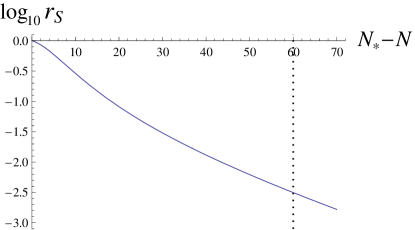
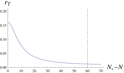
Figure 2: The evolutions of correlation coefficient $\cos\Delta$ (upper graph), entropy-to-curvature ratio $r_{\mathcal{S}}$ (its logarithm, middle graph) and tensor-to-scalar ratio $r_{T}$ (lower graph) with respect to e-folding number $N_{\ast}-N$ after crossing the horizon. This figure is drawn according to the model with action (48). The vertical dotted black lines correspond to $N_{\ast}-N=60$. The horizontal dotted black line corresponds to $\cos\Delta=1$, that is, the totally correlated situation.

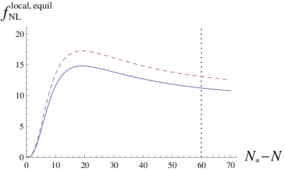
Figure 3: The evolutions of nonlinear parameters of curvature perturbation with respect to e-folding number $N_{\ast}-N$ after crossing the horizon. The solid blue line corresponds to the local limit value $f_{NL}^{local}$, while the dashed purple line depicts the nonlinear parameter of equilateral shape $f_{NL}^{equil}$. The vertical dotted black line corresponds to $N_{\ast}-N=60$. This figure is drawn according to the model with action (48).

For later convenience, let us define a new notation

$$\gamma=\frac{M_{p}^{2}}{\varphi^{2}}.$$ (49)

This notation is also useful in the next section. In the present case, one can prove

$$\epsilon_{1}+\eta_{1}\simeq-\frac{4M_{p}^{2}(3M_{p}^{4}+\varphi^{4})}{3(M_{p}^{2}+\varphi^{2})^{3}}.$$ (50)

According to this expression, the condition $\gamma\ll 1$ is necessary in order to satisfy the slow-roll conditions. As will be clear below, this is also the sufficient condition to meet the slow-roll conditions. So we can conclude that this model describes the large field inflation.

All of the slow-roll parameters can be expressed in terms of $\gamma$ to the leading order as

$$\epsilon_{1}=\frac{\dot{H}}{H^{2}}\simeq-\frac{4}{3}\gamma,\leavevmode\nobreak\ \leavevmode\nobreak\ \leavevmode\nobreak\ \leavevmode\nobreak\ \eta_{1}=\frac{\ddot{\varphi}}{H\dot{\varphi}}\simeq 4\gamma^{2},\leavevmode\nobreak\ \leavevmode\nobreak\ \leavevmode\nobreak\ \leavevmode\nobreak\ \delta_{1}=\frac{\dot{F}}{HF}\simeq\frac{8}{3}\gamma^{2},$$

$$\delta_{2}=\frac{\dot{E}}{HE}\simeq-\frac{4}{3}\gamma,\leavevmode\nobreak\ \leavevmode\nobreak\ \leavevmode\nobreak\ \leavevmode\nobreak\ \delta_{3}=\frac{\ddot{F}}{H\dot{F}}\simeq 4\gamma,\leavevmode\nobreak\ \leavevmode\nobreak\ \leavevmode\nobreak\ \leavevmode\nobreak\ \delta_{4}=\frac{\ddot{E}}{H\dot{E}}\simeq 4\gamma^{2},$$

$$\epsilon_{2}=\frac{\ddot{H}}{H\dot{H}}\simeq\frac{8}{3}\gamma^{2},\leavevmode\nobreak\ \leavevmode\nobreak\ \leavevmode\nobreak\ \leavevmode\nobreak\ \eta_{2}=\frac{\dddot{\varphi}}{H\ddot{\varphi}}\simeq 4\gamma,\leavevmode\nobreak\ \leavevmode\nobreak\ \leavevmode\nobreak\ \leavevmode\nobreak\ \delta_{6}=\frac{\dddot{E}}{H\ddot{E}}\simeq 4\gamma.$$ (51)

The coefficients (II) are

$$\frac{m_{\mathcal{R}}^{2}}{H^{2}}\simeq-\frac{8}{3}\gamma, \beta\simeq-2\sqrt{\frac{2\gamma}{3}},$$

$$\alpha\simeq-\frac{4}{3}\sqrt{\frac{2\gamma}{3}}, \frac{m_{\mathcal{S}}^{2}}{H^{2}}\simeq-2+8\gamma.$$ (52)

When the perturbations cross the horizon,

$$\mathcal{P}_{\mathcal{R}\ast}=\mathcal{P}_{\mathcal{S}\ast}=\frac{3m^{2}\varphi_{\ast}^{4}}{256\pi^{2}M_{p}^{6}},$$

$$r_{\mathcal{S}\ast}=1,\leavevmode\nobreak\ \leavevmode\nobreak\ \leavevmode\nobreak\ \leavevmode\nobreak\ n_{\mathcal{R}\ast}-1=n_{\mathcal{S}\ast}-1=-\frac{16}{3}\gamma_{\ast},$$

$$\mu_{\mathcal{S}\ast}=-\frac{32}{3}\gamma_{\ast},\leavevmode\nobreak\ \leavevmode\nobreak\ \leavevmode\nobreak\ \leavevmode\nobreak\ \mu_{\mathcal{R}\ast}=\frac{4}{3}\sqrt{\gamma_{\ast}},$$

$$\xi_{\ast}=\sqrt{2}\gamma_{\ast}^{\frac{3}{2}},\leavevmode\nobreak\ \leavevmode\nobreak\ \leavevmode\nobreak\ \leavevmode\nobreak\ \left.\frac{\dot{\xi}}{H\xi}\right|_{\ast}=4\gamma_{\ast}.$$ (53)

If we use the horizon-crossing value to estimate $\mu_{\mathcal{S}}$ and $\mu_{\mathcal{R}}$ outside the horizon, then at the end of inflation ($N=0$),

$$\frac{\mathcal{P}_{\mathcal{R}}}{\mathcal{P}_{\mathcal{S}\ast}}=\frac{9}{64\gamma_{\ast}}\left(1-e^{-32N_{\ast}\gamma_{\ast}/9}\right)^{2}+1,$$

$$\frac{\mathcal{P}_{\mathcal{S}}}{\mathcal{P}_{\mathcal{S}\ast}}=e^{-64N_{\ast}\gamma_{\ast}/9},\leavevmode\nobreak\ \leavevmode\nobreak\ \leavevmode\nobreak\ \leavevmode\nobreak\ \frac{\mathcal{P}_{T}}{\mathcal{P}_{\mathcal{S}\ast}}=\frac{64}{3}\gamma_{\ast},$$

$$\frac{\mathcal{P}_{\mathcal{C}}}{\mathcal{P}_{\mathcal{S}\ast}}=\frac{3}{8\sqrt{\gamma_{\ast}}}e^{-32N_{\ast}\gamma_{\ast}/9}\left(1-e^{-32N_{\ast}\gamma_{\ast}/9}\right),$$

$$n_{\mathcal{R}}-1=-\frac{16}{3}\gamma_{\ast},\leavevmode\nobreak\ \leavevmode\nobreak\ \leavevmode\nobreak\ \leavevmode\nobreak\ n_{\mathcal{S}}-1=\frac{16}{9}\gamma_{\ast},$$

$$n_{\mathcal{C}}-1=\frac{16}{3}\gamma_{\ast},\leavevmode\nobreak\ \leavevmode\nobreak\ \leavevmode\nobreak\ \leavevmode\nobreak\ n_{T}=-\frac{8}{3}\gamma_{\ast}.$$ (54)

To determine the parameter $\gamma_{\ast}$, we make use of the observational constraint on curvature spectral index $n_{\mathcal{R}}-1\simeq-0.04$, which gives approximately $\gamma_{\ast}=3/400$. The results are shown in figures 1 and figure 2. In figure 1 we plot the evolution of spectra $\mathcal{P}_{\mathcal{R}}$, $\mathcal{P}_{\mathcal{S}}$, $\mathcal{P}_{\mathcal{C}}$ and $\mathcal{P}_{T}$, which are defined in (II), (15) and (22). When drawing the graph, we have normalized them by $\mathcal{P}_{\mathcal{S}\ast}$. Figure 2 depicts the evolution of the correlation coefficient $\cos\Delta$, the logarithm of entropy-to-curvature ratio $r_{\mathcal{S}}$ and the tensor-to-scalar ratio $r_{T}$, defined by (21) and (24).

At the end of inflation, it can be seen from figure 2 that the entropy perturbation and the curvature perturbation are almost totally correlated, and the entropy-to-curvature ratio $r_{\mathcal{S}}$ is of order $10^{-3}$. At first glance, the entropy-to-curvature ratio here can be tested against WMAP5 constraint Komatsu:2008hk as done by Ji:2009yw . However, this is a misleading game. What WMAP5 constrained is the entropy perturbation

$$\mathcal{S}_{c,\gamma}=\frac{\delta\rho_{c}}{\rho_{c}}-\frac{3\delta\rho_{\gamma}}{4\rho_{\gamma}}$$ (55)

between dark matter and radiation. In our model the entropy perturbation Ji:2009yw

$$\mathcal{S}\propto\frac{\delta\varphi}{\dot{\varphi}}-\frac{F}{\dot{F}}(\psi-\phi)$$ (56)

which is related to the difference between the Newtonian potential $\phi$ and the spatial curvature $\psi$. Firstly, the normalization of $\mathcal{S}$ does not match to $\mathcal{S}$. Second, it is unlikely that the two degrees of freedom in our model will decay into radiation and dark matter respectively. Most probably such an entropy perturbation would seed an anisotropic stress or quadrupole moments of photons and neutrinos. Third, the entropy mode may decay after inflation, which depends on the detailed mechanism of reheating. Especially, the entropy perturbation can be erased by thermal equilibrium of matter and radiation before the creation of any non-zero conserved quantum number Komatsu:2008hk ; Weinberg:2004kr ; Weinberg:2004kf .

To estimate the non-Gaussianity, we calculate (III) for the present case,

$$f_{NL}^{local} = \frac{40\left[2048\gamma_{\ast}^{3}+135\sqrt{2}\left(1-e^{-32N_{\ast}\gamma_{\ast}/9}\right)^{3}\right]}{9\left[64\gamma_{\ast}+9\left(1-e^{-32N_{\ast}\gamma_{\ast}/9}\right)^{2}\right]^{2}},$$

$$f_{NL}^{equil} = \frac{20\left[17408\gamma_{\ast}^{3}+945\sqrt{2}\left(1-e^{-32N_{\ast}\gamma_{\ast}/9}\right)^{3}\right]}{27\left[64\gamma_{\ast}+9\left(1-e^{-32N_{\ast}\gamma_{\ast}/9}\right)^{2}\right]^{2}}.$$ (57)

Once again we set $\gamma_{\ast}=3/400$, then the numerical result gives the nonlinear parameter $f_{NL}^{local}$ and $f_{NL}^{equil}$ as functions of the e-folding number $N_{\ast}$. Both of them are illustrated in figure 3. At the end of inflation, this model will give the nonlinear parameters $f_{NL}^{local}\simeq 11$ and $f_{NL}^{equil}\simeq 13$.

Although all of the above predictions (or postdictions) are consistent with observational data, this model suffers from a serious problem, as we want to point out here. If we take $n_{\mathcal{R}}-1=-0.04$, then the normalization of curvature power spectrum $\mathcal{P}_{\mathcal{R}}\sim 10^{-9}$ requires $m^{2}/M_{p}^{2}\sim 10^{-5}$. On the other hand, the smallness of cosmological constant requires $\mu^{2}/M_{p}^{2}\sim 10^{-121}$ in action (2). In other words, if one intends to use model (48) to explain the comic microwave background (CMB) anisotropy, the residual “dark energy” will be too large compared with the observed value. For this reason, we conclude the model (48) with a quadratic potential is unattractive. In section VII, we will discuss another problem of it.

VI Quartic Potential: $V(\varphi)=\lambda\varphi^{4}$

Starting with the action

$$S=\int d^{4}x\sqrt{-g}\left[\frac{1}{2}M_{p}^{2}R+\frac{4\lambda^{2}\varphi^{4}(\varphi^{4}-36M_{p}^{4})}{6M_{p}^{2}R}-\frac{1}{2}g^{\alpha\beta}\partial_{\alpha}\varphi\partial_{\beta}\varphi-\lambda\varphi^{4}\right],\leavevmode\nobreak\ \leavevmode\nobreak\ \leavevmode\nobreak\ \leavevmode\nobreak\ (\lambda>0)$$ (58)

the treatment of this model is similar to the previous section, but the result is more encouraging.

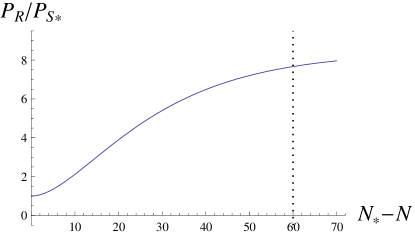
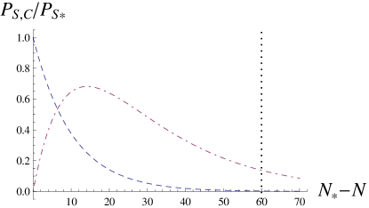
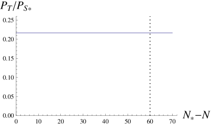
Figure 4: The evolutions of power spectra with respect to e-folding number $N_{\ast}-N$ after crossing the horizon. We draw this figure according to the model with action (58). The upper graph depicts the evolution of curvature power spectrum $\mathcal{P}_{\mathcal{R}}$. The middle graph depicts the evolution curves of entropy power spectrum $\mathcal{P}_{\mathcal{S}}$ (dashed blue line) and cross-correlation power spectrum $\mathcal{P}_{\mathcal{C}}$ (dot-dashed purple line). The lower corresponds to tensor power spectrum $\mathcal{P}_{T}$. All of the power spectra are normalized by $\mathcal{P}_{\mathcal{S\ast}}$, the entropy power spectrum at horizon-crossing. The vertical dotted black lines correspond to $N_{\ast}-N=60$.

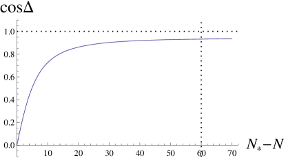
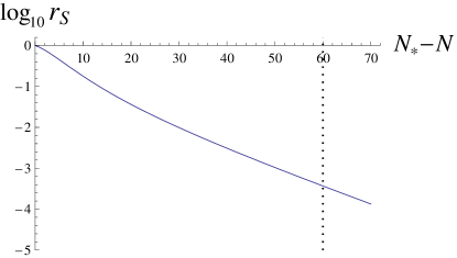
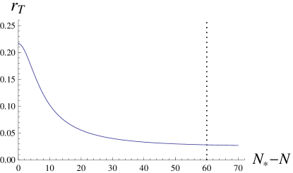
Figure 5: The evolutions of correlation coefficient $\cos\Delta$ (upper graph), entropy-to-curvature ratio $r_{\mathcal{S}}$ (its logarithm, middle graph) and tensor-to-scalar ratio $r_{T}$ (lower graph) with respect to e-folding number $N_{*}-N$ after crossing the horizon. This figure is drawn according to the model with action (58). The vertical dotted black lines correspond to $N_{*}-N=60$. The horizontal dotted black line corresponds to $\cos\Delta=-1$, that is, the totally anti-correlated situation.

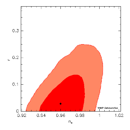
Figure 6: The black dot is the prediction of quartic model (58) for $n_{\mathcal{R}}$ and $r_{T}$, where we have set $\gamma_{\ast}=1/400$. It is consistent with the constraint from WMAP5 + BAO (baryon acoustic oscillations) + SN (supernovae) Komatsu:2008hk .

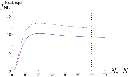
Figure 7: The evolutions of nonlinear parameters of curvature perturbation with respect to e-folding number $N_{\ast}-N$ after crossing the horizon. The solid blue curve corresponds to the local limit value $f_{NL}^{local}$, while the dashed purple curve plots the value in equilateral limit $f_{NL}^{equil}$. The vertical dotted black line corresponds to $N_{\ast}-N=60$. This figure is drawn according to the model with action (58).

Again we find the necessary condition $\gamma=M_{p}^{2}/\varphi^{2}\ll 1$ for slow-roll because of the relation

$$\epsilon_{1}+\eta_{1}\simeq-\frac{8M_{p}^{2}(72M_{p}^{6}+96M_{p}^{4}\varphi^{2}+16M_{p}^{2}\varphi^{4}+\varphi^{6})}{3\varphi^{2}(6M_{p}^{2}+\varphi^{2})^{3}}.$$ (59)

To the leading order of $\gamma$, we write the slow-roll parameters in the present case

$$\epsilon_{1}=\frac{\dot{H}}{H^{2}}\simeq-\frac{16}{3}\gamma,\leavevmode\nobreak\ \leavevmode\nobreak\ \leavevmode\nobreak\ \leavevmode\nobreak\ \eta_{1}=\frac{\ddot{\varphi}}{H\dot{\varphi}}\simeq-\frac{8}{3}\gamma,\leavevmode\nobreak\ \leavevmode\nobreak\ \leavevmode\nobreak\ \leavevmode\nobreak\ \delta_{1}=\frac{\dot{F}}{HF}\simeq 32\gamma^{2},$$

$$\delta_{2}=\frac{\dot{E}}{HE}\simeq-\frac{16}{3}\gamma,\leavevmode\nobreak\ \leavevmode\nobreak\ \leavevmode\nobreak\ \leavevmode\nobreak\ \delta_{3}=\frac{\ddot{F}}{H\dot{F}}\simeq\frac{16}{3}\gamma,\leavevmode\nobreak\ \leavevmode\nobreak\ \leavevmode\nobreak\ \leavevmode\nobreak\ \delta_{4}=\frac{\ddot{E}}{H\dot{E}}\simeq-\frac{16}{3}\gamma,$$

$$\epsilon_{2}=\frac{\ddot{H}}{H\dot{H}}\simeq-\frac{16}{3}\gamma^{2},\leavevmode\nobreak\ \leavevmode\nobreak\ \leavevmode\nobreak\ \leavevmode\nobreak\ \eta_{2}=\frac{\dddot{\varphi}}{H\ddot{\varphi}}\simeq-\frac{8}{3}\gamma,\leavevmode\nobreak\ \leavevmode\nobreak\ \leavevmode\nobreak\ \leavevmode\nobreak\ \delta_{6}=\frac{\dddot{E}}{H\ddot{E}}\simeq-\frac{16}{3}\gamma.$$ (60)

and the coefficients (II) for evolution equations,

$$\frac{m_{\mathcal{R}}^{2}}{H^{2}}\simeq-8\gamma, \beta\simeq-4\sqrt{\frac{2\gamma}{3}},$$

$$\alpha\simeq-\frac{8}{3}\sqrt{\frac{2\gamma}{3}}, \frac{m_{\mathcal{S}}^{2}}{H^{2}}\simeq-2+56\gamma.$$ (61)

When the perturbations cross the horizon,

$$\mathcal{P}_{\mathcal{R}\ast}=\mathcal{P}_{\mathcal{S}\ast}=\frac{3\lambda\varphi_{\ast}^{6}}{512\pi^{2}M_{p}^{6}},$$

$$r_{\mathcal{S}\ast}=1,\leavevmode\nobreak\ \leavevmode\nobreak\ \leavevmode\nobreak\ \leavevmode\nobreak\ n_{\mathcal{R}\ast}-1=n_{\mathcal{S}\ast}-1=-16\gamma_{\ast},$$

$$\mu_{\mathcal{S}\ast}=-\frac{176}{9}\gamma_{\ast},\leavevmode\nobreak\ \leavevmode\nobreak\ \leavevmode\nobreak\ \leavevmode\nobreak\ \mu_{\mathcal{R}\ast}=\frac{8}{3}\sqrt{\gamma_{\ast}},$$

$$\xi_{\ast}=6\sqrt{2}\gamma_{\ast}^{\frac{3}{2}},\leavevmode\nobreak\ \leavevmode\nobreak\ \leavevmode\nobreak\ \leavevmode\nobreak\ \left.\frac{\dot{\xi}}{H\xi}\right|_{\ast}=8\gamma_{\ast}.$$ (62)

If we use the horizon-crossing value to estimate $\mu_{\mathcal{S}}$ and $\mu_{\mathcal{R}}$ outside the horizon, then at the end of inflation ($N=0$), the power spectra and spectral indices are

$$\frac{\mathcal{P}_{\mathcal{R}}}{\mathcal{P}_{\mathcal{S}\ast}}=\frac{9}{484\gamma_{\ast}}\left(1-e^{-176N_{\ast}\gamma_{\ast}/9}\right)^{2}+1,$$

$$\frac{\mathcal{P}_{\mathcal{S}}}{\mathcal{P}_{\mathcal{S}\ast}}=e^{-352N_{\ast}\gamma_{\ast}/9},\leavevmode\nobreak\ \leavevmode\nobreak\ \leavevmode\nobreak\ \leavevmode\nobreak\ \frac{\mathcal{P}_{T}}{\mathcal{P}_{\mathcal{S}\ast}}=\frac{256}{3}\gamma_{\ast},$$

$$\frac{\mathcal{P}_{\mathcal{C}}}{\mathcal{P}_{\mathcal{S}\ast}}=\frac{3}{22\sqrt{\gamma_{\ast}}}e^{-176N_{\ast}\gamma_{\ast}/9}\left(1-e^{-176N_{\ast}\gamma_{\ast}/9}\right),$$

$$n_{\mathcal{R}}-1=-16\gamma_{\ast},\leavevmode\nobreak\ \leavevmode\nobreak\ \leavevmode\nobreak\ \leavevmode\nobreak\ n_{\mathcal{S}}-1=\frac{208}{9}\gamma_{\ast},$$

$$n_{\mathcal{C}}-1=\frac{128}{3}\gamma_{\ast},\leavevmode\nobreak\ \leavevmode\nobreak\ \leavevmode\nobreak\ \leavevmode\nobreak\ n_{T}=-\frac{32}{3}\gamma_{\ast}.$$ (63)

From the horizon-crossing to the end of inflation, the power spectrum of curvature perturbation has increased significantly. In sharp contrast, the entropy perturbation drops down exponentially with respect to $N_{\ast}-N$. The cross-correlation between them takes a positive value, at first increasing in amplitude and then decreasing. As we have promised, the tensor type perturbation is invariant. These results are presented in figure 4.

Now turn to figure 5. Look at the upper graph for the evolution of correlation coefficient $\cos\Delta$. Under our approximation, at the time of Hubble-crossing ($N_{\ast}-N=0$), the curvature perturbation and the entropy perturbation are uncorrelated. But the the subsequent evolution makes them almost totally correlated at the end of inflation ($N_{\ast}-N=60$).

From the lower graph of figure 5, it is clear that the tensor-to-scalar ratio is depressed greatly even at the horizon-crossing time (compared with the $\lambda\varphi^{4}$ inflation in Einstein gravity). Let us take a closer look on this point. Given the choice (46), at the time of Hubble-crossing, the power spectrum for curvature perturbation and that for tensor type perturbation can be written as

$$\mathcal{P}_{\mathcal{R}\ast}=\frac{3V^{3}}{32\pi^{2}M_{p}^{6}V_{,\varphi}^{2}},\leavevmode\nobreak\ \leavevmode\nobreak\ \leavevmode\nobreak\ \leavevmode\nobreak\ \mathcal{P}_{T\ast}=\frac{V}{2\pi^{2}M_{p}^{2}}.$$ (64)

In contrast, the counterparts in Einstein gravity are given by

$$\mathcal{P}_{\mathcal{R}}|_{\mathrm{Einstein}}=\frac{V^{3}}{12\pi^{2}M_{p}^{6}V_{,\varphi}^{2}},\leavevmode\nobreak\ \leavevmode\nobreak\ \leavevmode\nobreak\ \leavevmode\nobreak\ \mathcal{P}_{T}|_{\mathrm{Einstein}}=\frac{2V}{3\pi^{2}M_{p}^{2}}.$$ (65)

The difference between (64) and (65) explains the smallness of $r_{T}$ at the horizon-crossing in our model. Outside the horizon, since the curvature perturbation is increasing while the tensor type perturbation is conserved, the value of $r_{T}$ becomes smaller and smaller. At the end of inflation, we have $r_{T}\simeq 0.03$. This is well inside the constraint of WMAP5 Komatsu:2008hk , as illustrated in figure 6.

Words are needed here about the entropy-to-curvature ratio $r_{\mathcal{S}}$, which is depicted in the middle graph of figure 5. Thanks to the exponential decrease of entropy perturbation, the value of $r_{\mathcal{S}}$ is of order $10^{-4}$ at the end of inflation, which is smaller than the WMAP5 upper bound Komatsu:2008hk . However, as we have emphasized in the previous section, it is not quite reasonable to compare the entropy perturbation here with that in WMAP5 result. A more relevant constraint might come from the quadrupole moments of neutrinos. Especially, since the entropy perturbation is very small at the end of inflation, we can treat $\phi+\psi$ as almost constant at that time. From equation (II), this gives

$$\psi-\phi=\frac{\dot{F}(2HF+\dot{F})}{2F\dot{\varphi}^{2}+3\dot{F}^{2}}(\phi+\psi)\propto\gamma_{\ast}\psi$$ (66)

in our specific model. It is an interesting question to investigate the implication of residual difference between spatial curvature and Newtonian potential. But we do not pursue it furthermore in this paper.

The non-Gaussian features can be studied as before. By virtue of the new relations between the slow-roll parameters and $\gamma_{\ast}$ we have

$$f_{NL}^{local} = \frac{220\left[21296\gamma_{\ast}^{3}+9\sqrt{2}\left(1-e^{-176N_{\ast}\gamma_{\ast}/9}\right)^{3}\right]}{3\left[484\gamma_{\ast}+9\left(1-e^{-176N_{\ast}\gamma_{\ast}/9}\right)^{2}\right]^{2}},$$

$$f_{NL}^{equil} = \frac{110\left[596288\gamma_{\ast}^{3}+207\sqrt{2}\left(1-e^{-176N_{\ast}\gamma_{\ast}/9}\right)^{3}\right]}{27\left[484\gamma_{\ast}+9\left(1-e^{-176N_{\ast}\gamma_{\ast}/9}\right)^{2}\right]^{2}}.$$ (67)

One can plot the evolution of $f_{NL}^{local}$ and $f_{NL}^{equil}$ with respect to $N_{\ast}-N$ in figure 7. At the end of inflation, this model will give the nonlinear parameters $f_{NL}^{local}\simeq 9$ and $f_{NL}^{equil}\simeq 12$. Of course, these numbers are just results of semi-quantitative estimation. If we take them seriously, we would like to compare them with observational constraints Komatsu:2008hk . They perfectly satisfy the WMAP5 limit $-9<f_{NL}^{local}<111$ and $-151<f_{NL}^{equil}<253$.

VII Stability Analysis

For model (1) in the large curvature region, due to the $1/R$ suppression, the correction term has negligible effects in the early universe if $\mu$ is small Carroll:2003wy . But recent investigations Song:2006ej ; Sawicki:2007tf showed that such correction terms may introduce instabilities, hence their effects are not negligible even in the high redshift epoch. So it is important to study the stability problem in our model (2). Since the inflaton field is evolving, and there is a signature change in $g(\varphi)$ around the end of inflation, we should study this problem during inflation and after reheating respectively.

To analyze the stability, there is an indicator $B$ given by formula (17) in Song:2006ej and formula (2) in Sawicki:2007tf . According to the results of Song:2006ej ; Sawicki:2007tf , the instability resides in the branch of models with $B<0$. We find for our model of the form (2), the indicator

$$B=\frac{2g}{M_{p}^{2}R^{2}-g}\frac{d\ln R}{d\ln a}\left(\frac{d\ln H}{d\ln a}\right)^{-1}.$$ (68)

During inflation, for $g$ taking the form (46) and $M_{p}^{2}V_{,\varphi\varphi}\ll V$, we get $B\simeq 2>0$, so the model is stable. This can also be inferred simply from the fact that $g>0$ during inflation.

As the inflaton rolled down the potential and decayed long after the inflation, for the quadratic and quartic potentials, we have $V\ll M_{p}^{2}V_{,\varphi\varphi}$ and then

$$B=-\frac{2V_{,\varphi\varphi}^{2}}{3R^{2}+V_{,\varphi\varphi}^{2}}\frac{d\ln R}{d\ln a}\left(\frac{d\ln H}{d\ln a}\right)^{-1}\leq 0.$$ (69)

The inequality is saturated if and only if $V_{,\varphi\varphi}=0$. This cannot happen when $V=\frac{1}{2}m^{2}\varphi^{2}$ because it always gives $V_{,\varphi\varphi}=m^{2}>0$. As a result, it does not have a proper matter-dominated phase. This is another problem of the model with a quadratic potential, as we have promised at the end of section VI.

But the story is a little different for the case $V=\lambda\varphi^{4}$, in which the unstable branch with $B<0$ can be avoided if the inflaton decayed to the minimum of its potential $\varphi=0$ during the reheating era. Therefore, the stability condition for the quartic potential model puts a constraint on reheating: the reheating process should to efficient enough to guarantee a complete decay of inflaton $\varphi$. Such an efficient decay can be realized most easily by the instant preheating mechanism Felder:1998vq . After the complete decay of $\varphi$ during reheating, the $f(\varphi,R)$ model of the form (58) is reduced to the Einstein gravity without any harmful instability in subsequent epochs.

The stability condition makes our models less interesting. Were the stability condition ignored, one might drive the acceleration of late universe with the residual non-vanishing inflaton, and thus unify the two phases of accelerated expansion of the universe with a single non-minimally coupled scalar field. After imposing the stability condition, there is no room for such a natural unification.

Of course, inspired by the so-called mCDTT model in Sawicki:2007tf , one may replace $g(\varphi)$ with $g(\varphi)+\mu^{4}M_{p}^{2}$ in (2), where $\mu\ll M_{p}$ is a constant independent of $\varphi$. Then the newly added term will play a role after inflation, exactly recover so-called mCDTT model, which can avoid the instability problem. But, since the constant $\mu$ is very small, this term plays no role during inflation. Moreover, as was advocated in Amendola:2006kh , all $f(R)$ modified gravity during the matter phase is grossly inconsistent with cosmological observations. So it seems that the only choice for us is to recover Einstein gravity after reheating.

Therefore, although we started with the $f(R)$ model and the accelerated expansion of late universe, due to various difficulties put forward in Amendola:2006kh ; Amendola:2006eh ; Song:2006ej ; Sawicki:2007tf , it turns out that our model has nothing to do with the $f(R)$ model at the late time. In other words, the survived $f(\varphi,R)$ inflation model should reduce to the Einstein gravity after reheating.

In contrast with Amendola:2006kh ; Amendola:2006eh , different viewpoints are held by the authors of Nojiri:2003ft ; Nojiri:2006gh ; Capozziello:2006dj . Interested readers may refine the analysis above by taking Nojiri:2003ft ; Nojiri:2006gh ; Capozziello:2006dj into consideration.

According to Corda:2007hi ; Corda:2009re , the interferometric detection of gravitational waves can provide a definitive test for general relativity. In other words, the interferometric detection of gravitational waves will be a strong endorsement for the modified gravity theories or, alternatively, will rule out them. So it would be also necessary to further inspect the $f(\varphi,R)$ models from this angle of view in the future.

VIII Comments and Conclusion

As we have stressed, our analysis throughout this paper is not more than a semi-quantitative estimation. Before concluding, we would like to remark on several weaknesses and the resulted uncertainties in the above calculations. We can classify them into three categories: the decoupled approximation inside the horizon, the linear evolution approximation outside the horizon and the slow-roll approximation.

First, as revealed by equations (II), the curvature perturbation and the entropy perturbation are coupled inside the horizon. But when writing down the analytical solution (II), we have neglected the coupling terms. As a subsequence, the correlation functions $\langle\mathcal{R}_{\ast}\mathcal{S}_{\ast}\rangle$, $\langle\mathcal{R}_{\ast}\mathcal{R}_{\ast}\mathcal{S}_{\ast}\rangle$ and $\langle\mathcal{R}_{\ast}\mathcal{S}_{\ast}\mathcal{S}_{\ast}\rangle$ vanish only because we have neglected the coupling between $\mathcal{R}_{\ast}$ and $\mathcal{S}_{\ast}$ inside the horizon. All of the power spectra and three point functions at the horizon-crossing should receive a correction from the coupling effects. The correction is controlled by coupling coefficients $\alpha$ and $\beta$ in evolution equations (II). This is also a general problem for analytical solution of multi-field inflation models. For a more accurate treatment to this problem in two-field inflation, please refer to Byrnes:2006fr .

Second, in deriving the transfer relation (II), we have neglected the nonlinear effects. As mentioned in section III, there are two sources of nonlinear effects outside the horizon: the $\ddot{S}_{k}$ term neglected in equation (II); the time dependence of $\mu_{\mathcal{S}}$ and $\mu_{\mathcal{R}}$. Again, this is also a general problem for analytical solution of multi-field inflation models.

Third, there is an additional source of uncertainty for the model studied in section IV, where we have deliberately kept the $V_{,\varphi\varphi}$ term in the Lagrangian. This is necessary to avoid the divergence of power spectrum at the leading order, but it brings some inconsistency for our slow-roll approximation. This is clear from equations (V) and (VI), in which the slow-roll parameters are not of the same order. In principle, this problem should be solved by doing the calculations at the sub-leading order in a consistent way. But the background dynamics will be rather messy, neither analytical nor numerical method can give it a hand.

Although the analytic results obtained in this paper are not accurate, it is still meaningful to take them for rough estimate before painstaking calculation. There are some lessons we can learn from it. For the $1/R$-corrected inflation, the evolution of entropy perturbation can dramatically depress the tensor-to-scalar ratio and enhance the magnitude of non-Gaussianity. Specifically, if we take the rough estimation seriously, then the single-field inflation can be rescued by the $1/R$ correction, otherwise it would have been excluded by observational data.

The preliminary investigation in Ji:2009yw and here raises more questions than answers about generalized $f(\varphi,R)$ gravity theories. First, we lack a first principle to write down the exact form of $f(\varphi,R)$ when higher or lower order corrections are considered. Second, all of the calculation makes sense only semi-quantitatively, so a more accurate treatment is in demand. The formalism we developed is applicable to other cosmological stages and scenarios. Especially, it would be interesting to find a unified model similar to Liddle:2008bm , but with richer phenomena. Third, it is possible that the entropy perturbation in $f(\varphi,R)$ inflation can seed a tiny quadruple moment of neutrinos, which deserves a detailed analysis. Fourth, according to our rough estimate, the non-Gaussianity is large and positive in some models. This is observationally interesting and should be studied carefully in the future.

Appendix A Three-Point Correlations of the Local Form

Before engaging ourselves in calculation, we notice that the definition of $\mathcal{R}_{k}$ and $\mathcal{S}_{k}$ in the text is

$$\mathcal{R}(\mathbf{x},t)=\int\frac{d^{3}\mathbf{k}}{(2\pi)^{\frac{3}{2}}}e^{i\mathbf{k}\cdot\mathbf{x}}\mathcal{R}_{\mathbf{k}}(t),\leavevmode\nobreak\ \leavevmode\nobreak\ \leavevmode\nobreak\ \leavevmode\nobreak\ \mathcal{S}(\mathbf{x},t)=\int\frac{d^{3}\mathbf{k}}{(2\pi)^{\frac{3}{2}}}e^{i\mathbf{k}\cdot\mathbf{x}}\mathcal{S}_{\mathbf{k}}(t).$$ (70)

But in calculating non-Gaussianity, usually a different normalization is followed,

$$\mathcal{R}(\mathbf{x},t)=\int\frac{d^{3}\mathbf{k}}{(2\pi)^{3}}e^{i\mathbf{k}\cdot\mathbf{x}}\tilde{\mathcal{R}}_{\mathbf{k}}(t),\leavevmode\nobreak\ \leavevmode\nobreak\ \leavevmode\nobreak\ \leavevmode\nobreak\ \mathcal{S}(\mathbf{x},t)=\int\frac{d^{3}\mathbf{k}}{(2\pi)^{3}}e^{i\mathbf{k}\cdot\mathbf{x}}\tilde{\mathcal{S}}_{\mathbf{k}}(t).$$ (71)

In terms of $\tilde{\mathcal{R}}_{k}$ and $\tilde{\mathcal{S}}_{k}$, we have the following relations between two-point correlations and power spectra Komatsu:2001rj ; Komatsu:2002db :

$$\langle\tilde{\mathcal{R}}_{\mathbf{k}1}\tilde{\mathcal{R}}_{\mathbf{k}2}\rangle=\frac{2\pi^{2}}{k^{3}}\tilde{\mathcal{P}}_{\mathcal{R}}(k)\delta(\mathbf{k}_{1}-\mathbf{k}_{2})=\frac{(2\pi)^{5}}{2k^{3}}\mathcal{P}_{\mathcal{R}}(k)\delta(\mathbf{k}_{1}-\mathbf{k}_{2}),$$

$$\langle\tilde{\mathcal{S}}_{\mathbf{k}1}\tilde{\mathcal{S}}_{\mathbf{k}2}\rangle=\frac{2\pi^{2}}{k^{3}}\tilde{\mathcal{P}}_{\mathcal{S}}(k)\delta(\mathbf{k}_{1}-\mathbf{k}_{2})=\frac{(2\pi)^{5}}{2k^{3}}\mathcal{P}_{\mathcal{S}}(k)\delta(\mathbf{k}_{1}-\mathbf{k}_{2}),$$

$$\langle\tilde{\mathcal{R}}_{\mathbf{k}1}\tilde{\mathcal{S}}_{\mathbf{k}2}\rangle=\frac{2\pi^{2}}{k^{3}}\tilde{\mathcal{C}}(k)\delta(\mathbf{k}_{1}-\mathbf{k}_{2})=\frac{(2\pi)^{5}}{2k^{3}}\mathcal{C}(k)\delta(\mathbf{k}_{1}-\mathbf{k}_{2}),$$

$$\langle\tilde{\mathcal{R}}(\mathbf{x}_{1},t)\tilde{\mathcal{R}}(\mathbf{x}_{2},t)\rangle=\int\frac{d^{3}\mathbf{k}}{4\pi k^{3}}\mathcal{P}_{\mathcal{R}}(k)e^{i\mathbf{k}\cdot(\mathbf{x}_{1}-\mathbf{x}_{2})},$$

$$\langle\tilde{\mathcal{S}}(\mathbf{x}_{1},t)\tilde{\mathcal{S}}(\mathbf{x}_{2},t)\rangle=\int\frac{d^{3}\mathbf{k}}{4\pi k^{3}}\mathcal{P}_{\mathcal{S}}(k)e^{i\mathbf{k}\cdot(\mathbf{x}_{1}-\mathbf{x}_{2})},$$

$$\langle\tilde{\mathcal{R}}(\mathbf{x}_{1},t)\tilde{\mathcal{S}}(\mathbf{x}_{2},t)\rangle=\int\frac{d^{3}\mathbf{k}}{4\pi k^{3}}\mathcal{P}_{\mathcal{C}}(k)e^{i\mathbf{k}\cdot(\mathbf{x}_{1}-\mathbf{x}_{2})}.$$ (72)

In accordance with the WMAP convention Komatsu:2008hk ; Komatsu:2001rj , we parameterize the nonlinearities of curvature and entropy perturbations as

$$\mathcal{R}(\mathbf{x},t) = \mathcal{R}_{L}-\frac{3}{5}f_{NL}^{\mathcal{R}}\left(\mathcal{R}_{L}^{2}-\langle\mathcal{R}_{L}^{2}\rangle\right),$$

$$\mathcal{S}(\mathbf{x},t) = \mathcal{S}_{L}-\frac{3}{5}f_{NL}^{\mathcal{S}}\left(\mathcal{S}_{L}^{2}-\langle\mathcal{S}_{L}^{2}\rangle\right).$$ (73)

Here $\mathcal{R}_{L}$ and $\mathcal{S}_{L}$ are linear Gaussian parts of the perturbations. If we take nonlinear parameters $f_{NL}^{\mathcal{R}}$ and $f_{NL}^{\mathcal{S}}$ as constants, then this is a local form non-Gaussianity, which can be written in the Fourier space as

$$\tilde{\mathcal{R}}(\mathbf{k}) = \tilde{\mathcal{R}}_{L}(\mathbf{k})-\frac{3}{5}f_{NL}^{\mathcal{R}}\left[\int\frac{d^{3}\mathbf{p}}{(2\pi)^{3}}\tilde{\mathcal{R}}_{L}(\mathbf{k}-\mathbf{p})\tilde{\mathcal{R}}_{L}(\mathbf{p})-\int d^{3}\mathbf{x}e^{-i\mathbf{k}\cdot\mathbf{x}}\langle\tilde{\mathcal{R}}_{L}^{2}(\mathbf{x})\rangle\right],$$

$$\tilde{\mathcal{S}}(\mathbf{k}) = \tilde{\mathcal{S}}_{L}(\mathbf{k})-\frac{3}{5}f_{NL}^{\mathcal{S}}\left[\int\frac{d^{3}\mathbf{p}}{(2\pi)^{3}}\tilde{\mathcal{S}}_{L}(\mathbf{k}-\mathbf{p})\tilde{\mathcal{S}}_{L}(\mathbf{p})-\int d^{3}\mathbf{x}e^{-i\mathbf{k}\cdot\mathbf{x}}\langle\tilde{\mathcal{S}}_{L}^{2}(\mathbf{x})\rangle\right].$$ (74)

$\langle\mathcal{R}_{L}^{2}\rangle$ and $\langle\mathcal{S}_{L}^{2}\rangle$ are counter terms to ensure $\langle\mathcal{R}(\mathbf{x},t)\rangle=\langle\mathcal{S}(\mathbf{x},t)\rangle=0$.

Using the above relations, it is straightforward to prove equation (30) and

$$\langle\tilde{\mathcal{R}}(\mathbf{k}_{1})\tilde{\mathcal{R}}(\mathbf{k}_{2})\tilde{\mathcal{S}}(\mathbf{k}_{3})\rangle$$ (75)

$$= -\frac{3}{5}f_{NL}^{\mathcal{R}}\int\frac{d^{3}\mathbf{p}}{(2\pi)^{3}}\langle\tilde{\mathcal{R}}_{L}(\mathbf{k}_{1}-\mathbf{p})\tilde{\mathcal{R}}_{L}(\mathbf{p})\tilde{\mathcal{R}}_{L}(\mathbf{k}_{2})\tilde{\mathcal{S}}_{L}(\mathbf{k}_{3})\rangle$$

$$-\frac{3}{5}f_{NL}^{\mathcal{R}}\int\frac{d^{3}\mathbf{p}}{(2\pi)^{3}}\langle\tilde{\mathcal{R}}_{L}(\mathbf{k}_{1})\tilde{\mathcal{R}}_{L}(\mathbf{k}_{2}-\mathbf{p})\tilde{\mathcal{R}}_{L}(\mathbf{p})\tilde{\mathcal{S}}_{L}(\mathbf{k}_{3})\rangle$$

$$-\frac{3}{5}f_{NL}^{\mathcal{S}}\int\frac{d^{3}\mathbf{p}}{(2\pi)^{3}}\langle\tilde{\mathcal{R}}_{L}(\mathbf{k}_{1})\tilde{\mathcal{R}}_{L}(\mathbf{k}_{2})\tilde{\mathcal{S}}_{L}(\mathbf{k}_{3}-\mathbf{p})\tilde{\mathcal{S}}_{L}(\mathbf{p})\rangle$$

$$+\mathrm{divergent\leavevmode\nobreak\ counter\leavevmode\nobreak\ terms}$$

$$= -\frac{6}{5}f_{NL}^{\mathcal{R}}\int d\mathbf{x}_{1}d\mathbf{x}_{2}d\mathbf{x}_{3}e^{-i\mathbf{k}_{1}\cdot\mathbf{x}_{1}-i\mathbf{k}_{2}\cdot\mathbf{x}_{2}-i\mathbf{k}_{3}\cdot\mathbf{x}_{3}}\langle\mathcal{R}_{L}(\mathbf{x}_{1})\mathcal{R}_{L}(\mathbf{x}_{2})\rangle\langle\mathcal{R}_{L}(\mathbf{x}_{1})\mathcal{S}_{L}(\mathbf{x}_{3})\rangle$$

$$-\frac{6}{5}f_{NL}^{\mathcal{R}}\int d\mathbf{x}_{1}d\mathbf{x}_{2}d\mathbf{x}_{3}e^{-i\mathbf{k}_{1}\cdot\mathbf{x}_{1}-i\mathbf{k}_{2}\cdot\mathbf{x}_{2}-i\mathbf{k}_{3}\cdot\mathbf{x}_{3}}\langle\mathcal{R}_{L}(\mathbf{x}_{1})\mathcal{R}_{L}(\mathbf{x}_{2})\rangle\langle\mathcal{R}_{L}(\mathbf{x}_{2})\mathcal{S}_{L}(\mathbf{x}_{3})\rangle$$

$$-\frac{6}{5}f_{NL}^{\mathcal{S}}\int d\mathbf{x}_{1}d\mathbf{x}_{2}d\mathbf{x}_{3}e^{-i\mathbf{k}_{1}\cdot\mathbf{x}_{1}-i\mathbf{k}_{2}\cdot\mathbf{x}_{2}-i\mathbf{k}_{3}\cdot\mathbf{x}_{3}}\langle\mathcal{R}_{L}(\mathbf{x}_{1})\mathcal{S}_{L}(\mathbf{x}_{3})\rangle\langle\mathcal{R}_{L}(\mathbf{x}_{2})\mathcal{S}_{L}(\mathbf{x}_{3})\rangle$$

$$= -\frac{3}{10}(2\pi)^{7}f_{NL}^{\mathcal{R}}\frac{\mathcal{P}_{\mathcal{R}}(k_{2})}{k_{2}^{3}}\frac{\mathcal{P}_{\mathcal{C}}(k_{3})}{k_{3}^{3}}\delta^{(3)}(\mathbf{k}_{1}+\mathbf{k}_{2}+\mathbf{k}_{3})$$

$$-\frac{3}{10}(2\pi)^{7}f_{NL}^{\mathcal{R}}\frac{\mathcal{P}_{\mathcal{R}}(k_{1})}{k_{1}^{3}}\frac{\mathcal{P}_{\mathcal{C}}(k_{3})}{k_{3}^{3}}\delta^{(3)}(\mathbf{k}_{1}+\mathbf{k}_{2}+\mathbf{k}_{3})$$

$$-\frac{3}{10}(2\pi)^{7}f_{NL}^{\mathcal{S}}\frac{\mathcal{P}_{\mathcal{C}}(k_{1})}{k_{1}^{3}}\frac{\mathcal{P}_{\mathcal{C}}(k_{2})}{k_{2}^{3}}\delta^{(3)}(\mathbf{k}_{1}+\mathbf{k}_{2}+\mathbf{k}_{3}).$$

By exchanging $\mathcal{R}\leftrightarrow\mathcal{S}$, one directly writes down

$$\langle\tilde{\mathcal{S}}(\mathbf{k}_{1})\tilde{\mathcal{S}}(\mathbf{k}_{2})\tilde{\mathcal{R}}(\mathbf{k}_{3})\rangle$$ (76)

$$= -\frac{3}{10}(2\pi)^{7}f_{NL}^{\mathcal{S}}\frac{\mathcal{P}_{\mathcal{S}}(k_{2})}{k_{2}^{3}}\frac{\mathcal{P}_{\mathcal{C}}(k_{3})}{k_{3}^{3}}\delta^{(3)}(\mathbf{k}_{1}+\mathbf{k}_{2}+\mathbf{k}_{3})$$

$$-\frac{3}{10}(2\pi)^{7}f_{NL}^{\mathcal{S}}\frac{\mathcal{P}_{\mathcal{S}}(k_{1})}{k_{1}^{3}}\frac{\mathcal{P}_{\mathcal{C}}(k_{3})}{k_{3}^{3}}\delta^{(3)}(\mathbf{k}_{1}+\mathbf{k}_{2}+\mathbf{k}_{3})$$

$$-\frac{3}{10}(2\pi)^{7}f_{NL}^{\mathcal{R}}\frac{\mathcal{P}_{\mathcal{C}}(k_{1})}{k_{1}^{3}}\frac{\mathcal{P}_{\mathcal{C}}(k_{2})}{k_{2}^{3}}\delta^{(3)}(\mathbf{k}_{1}+\mathbf{k}_{2}+\mathbf{k}_{3}).$$

The above derivation is valid when $f_{NL}^{\mathcal{R}}$ and $f_{NL}^{\mathcal{S}}$ are constants. This is the case for the local shape non-Gaussianity. We hope the results can be generalized to other shapes as if $f_{NL}^{\mathcal{R}}$ and $f_{NL}^{\mathcal{S}}$ are $\mathbf{k}$-dependent. But this conjecture is to be proved or disproved by a more careful investigation in the future.

References

(1)
S. G. Turyshev,
Usp. Fiz. Nauk 179, 3 (2009)
[Phys. Usp. 52, 1 (2009)]
[arXiv:0809.3730 [gr-qc]].
(2)
A. G. Riess et al. [Supernova Search Team Collaboration],
Astron. J. 116, 1009 (1998)
[arXiv:astro-ph/9805201].
(3)
S. Perlmutter et al. [Supernova Cosmology Project Collaboration],
Astrophys. J. 517, 565 (1999)
[arXiv:astro-ph/9812133].
(4)
E. Komatsu et al. [WMAP Collaboration],
Astrophys. J. Suppl. 180, 330 (2009)
[arXiv:0803.0547 [astro-ph]].
(5)
G. R. Dvali, G. Gabadadze and M. Porrati,
Phys. Lett. B 485, 208 (2000)
[arXiv:hep-th/0005016].
(6)
S. M. Carroll, V. Duvvuri, M. Trodden and M. S. Turner,
Phys. Rev. D 70, 043528 (2004)
[arXiv:astro-ph/0306438].
(7)
M. Li,
Phys. Lett. B 603, 1 (2004)
[arXiv:hep-th/0403127].
(8)
S. Nojiri and S. D. Odintsov,
eConf C0602061, 06 (2006)
[Int. J. Geom. Meth. Mod. Phys. 4, 115 (2007)]
[arXiv:hep-th/0601213].
(9)
T. P. Sotiriou and V. Faraoni,
arXiv:0805.1726 [gr-qc].
(10)
X. d. Ji and T. Wang,
Phys. Rev. D 79, 103525 (2009)
[arXiv:0903.0379 [hep-th]].
(11)
L. Amendola, D. Polarski and S. Tsujikawa,
Phys. Rev. Lett. 98, 131302 (2007)
[arXiv:astro-ph/0603703].
(12)
L. Amendola, D. Polarski and S. Tsujikawa,
Int. J. Mod. Phys. D 16, 1555 (2007)
[arXiv:astro-ph/0605384].
(13)
Y. S. Song, W. Hu and I. Sawicki,
Phys. Rev. D 75, 044004 (2007)
[arXiv:astro-ph/0610532].
(14)
I. Sawicki and W. Hu,
Phys. Rev. D 75, 127502 (2007)
[arXiv:astro-ph/0702278].
(15)
S. Nesseris,
arXiv:0811.4292 [astro-ph].
(16)
J. Sadeghi, M. R. Setare and A. Banijamali,
arXiv:0903.4073 [hep-th].
(17)
O. Bertolami and M. C. Sequeira,
arXiv:0903.4540 [gr-qc].
(18)
Y. Ito and S. Nojiri,
arXiv:0904.0367 [hep-th].
(19)
A. R. Liddle, C. Pahud and L. A. Urena-Lopez,
Phys. Rev. D 77, 121301 (2008)
[arXiv:0804.0869 [astro-ph]].
(20)
J. C. Hwang,
Class. Quant. Grav. 7, 1613 (1990).
(21)
J. C. Hwang,
Class. Quant. Grav. 14, 1981 (1997)
[arXiv:gr-qc/9605024].
(22)
J. C. Hwang,
Class. Quant. Grav. 14, 3327 (1997)
[arXiv:gr-qc/9607059].
(23)
J. C. Hwang,
Class. Quant. Grav. 15, 1401 (1998)
[arXiv:gr-qc/9710061].
(24)
J. C. Hwang and H. Noh,
Phys. Rev. D 71, 063536 (2005)
[arXiv:gr-qc/0412126].
(25)
B. Chen, M. Li, T. Wang and Y. Wang,
Mod. Phys. Lett. A 22, 1987 (2007)
[arXiv:astro-ph/0610514].
(26)
E. Ramirez and D. J. Schwarz,
arXiv:0903.3543 [astro-ph.CO].
(27)
P. Teyssandier and Ph. Tourrenc,
J. Math. Phys. 24, 2793 (1983).
(28)
K. I. Maeda,
Phys. Rev. D 39, 3159 (1989).
(29)
D. Wands,
Class. Quant. Grav. 11, 269 (1994)
[arXiv:gr-qc/9307034].
(30)
T. Matsuda,
arXiv:0906.0643 [hep-th].
(31)
D. Wands, K. A. Malik, D. H. Lyth and A. R. Liddle,
Phys. Rev. D 62, 043527 (2000)
[arXiv:astro-ph/0003278].
(32)
D. Wands, N. Bartolo, S. Matarrese and A. Riotto,
Phys. Rev. D 66, 043520 (2002)
[arXiv:astro-ph/0205253].
(33)
D. Langlois,
Phys. Rev. D 59, 123512 (1999)
[arXiv:astro-ph/9906080].
(34)
E. Komatsu and D. N. Spergel,
Phys. Rev. D 63, 063002 (2001)
[arXiv:astro-ph/0005036].
(35)
X. Chen, M. x. Huang, S. Kachru and G. Shiu,
JCAP 0701, 002 (2007)
[arXiv:hep-th/0605045].
(36)
J. M. Maldacena,
JHEP 0305, 013 (2003)
[arXiv:astro-ph/0210603].
(37)
M. Li and Y. Wang,
JCAP 0809, 018 (2008)
[arXiv:0807.3058 [hep-th]].
(38)
E. Komatsu,
arXiv:astro-ph/0206039.
(39)
M. Li, T. Wang and Y. Wang,
JCAP 0803, 028 (2008)
[arXiv:0801.0040 [astro-ph]].
(40)
X. Chen, R. Easther and E. A. Lim,
JCAP 0804, 010 (2008)
[arXiv:0801.3295 [astro-ph]].
(41)
Q. G. Huang,
Phys. Lett. B 669, 260 (2008)
[arXiv:0801.0467 [hep-th]].
(42)
S. W. Li and W. Xue,
arXiv:0804.0574 [astro-ph].