Fluctuations in classical sum rules

Abstract

Classical sum rules arise in a wide variety of physical contexts. Asymptotic expressions have been derived for many of these sum rules in the limit of long orbital period (or large action). Although sum rule convergence may well be exponentially rapid for chaotic systems in a global sense with time, individual contributions to the sums may fluctuate with a width which diverges in time. Our interest is in the global convergence of sum rules as well as their local fluctuations. It turns out that a simple version of a lazy baker map gives an ideal system in which classical sum rules, their corrections, and their fluctuations can be worked out analytically. This is worked out in detail for the Hannay-Ozorio sum rule. In this particular case the rate of convergence of the sum rule is found to be governed by the Pollicott-Ruelle resonances, and both local and global boundaries for which the sum rule may converge are given. In addition, the width of the fluctuations is considered and worked out analytically, and it is shown to have an interesting dependence on the location of the region over which the sum rule is applied. It is also found that as the region of application is decreased in size the fluctuations grow. This suggests a way of controlling the length scale of the fluctuations by considering a time dependent phase space volume, which for the lazy baker map decreases exponentially rapidly with time.

I Introduction

Classical sum rules play an important role in a number of physical contexts. It is interesting to have a case of a non-uniformly spreading chaotic system where their limits, fluctuations, and convergences can be studied analytically, which is given in this paper. We focus on the sum rule of Hannay and Ozorio de Almeida, who were motivated by a desire to understand the two-point quantum density of states correlator Hannay and de Almeida (1984). Their derivation relied on the Principle of Uniformity, which states that the periodic orbits, weighted naturally are uniformly dense in phase space. There are many others; see, for example, the sum rules in Refs. Argaman (1996); Sieber (1999); Richter and Sieber (2002) which involve return probability, the connection of two points in coordinate space, and fixed orientations of initial and final velocities, respectively. They arise in mesoscopic conductance, diffraction contributions to spectral fluctuations, and chaotic quantum transport, also respectively.

In one possible form of the Hannay-Ozorio sum rule Ozorio de Almeida (1988) for chaotic systems, it is the inverses of the stability matrix determinants for the periodic orbits of period $\tau$, $\left|{\rm Det}\left({\mathbf{M}}_{\tau}-{\mathbf{1}}\right)\right|^{-1}$, which are summed. For completely chaotic systems the finite-time stability exponents, which roughly determine the value of each determinant, converge as $\tau\rightarrow\infty$ to a single set. Nevertheless, the determinant’s fluctuations from one periodic orbit to the next grow without bound in the same limit. This feature is made even more curious by the expectation that the Hannay-Ozorio sum rule converges exponentially rapidly. See a preprint by Pollicott Pollicott (2001) for a theorem regarding the sum rule’s convergence.

It is known that smooth classical functions have exponential decays in fully chaotic systems toward their ergodic averages, which are governed by the Pollicott-Ruelle (PR) resonances Pollicott (1985, 1986); Ruelle (1986, 1987) associated with the Perron-Frobenius operator. It is natural to ask whether the kinds of classical sum rules encountered always converge to their limiting values with corrections that decay exponentially according to the leading PR resonances. The work of Andreev et al. Andreev et al. (1996) would suggest that as long as there is a gap in the spectra of the Perron-Frobenius operators, there is no other possibility.

A first step is taken here in approaching this general line of questioning by considering a form of the Hannay-Ozorio sum rule for fixed period in maps. Its convergence rate and local fluctuations are considered in detail in a simple version of a lazy baker map introduced by Balazs and one of us (AL) Lakshminarayan and Balazs (1993); Lakshminarayan (1993). Although the usual baker map is especially simple, it is also non-generic in that its lacks the essential fluctuations of interest, whereas the lazy baker map possesses fluctuations and still turns out to be analytically tractable. The fluctuations of the inverse determinant were studied briefly in Ref. Tomsovic and Lakshminarayan (2007), where they were demonstrated, not surprisingly, to be extremely sensitive to even tiny islands of stability. In the form of the lazy baker map studied here, all orbits, with one exception of a marginal orbit of period two, are unstable, and there is no ambiguity concerning whether the system is completely chaotic.

The organization of this paper is as follows: in Sect. II notations are specified and definitions of various quantities of interest are given. Section III introduces a simple version of a lazy baker map (named the SR map), which is studied in detail, and gives basic counting results for fixed points and a method of subdividing the phase space into local regions. This is followed in Sect. IV by a derivation of the main results for the local fluctuation and convergence properties of the Hannay-Ozorio sum rule.

II Measurements of chaotic systems

Dynamical systems theory has generated a number of ways to specify the complexity of a chaotic mapping. Three of the more familiar concepts to physicists are the topological entropy, $h_{T}$, the metric or Kolmogorov-Sinai (KS) entropy, and the Lyapunov exponent, $\lambda_{L}$ Jacobs et al. (1998); Ott (2002). The topological entropy is designed to measure the information content of the optimal partition of the dynamics. It turns out for that a class of systems known as Axiom A, the limiting value of the exponential rate of increase in the number of fixed points with iteration number gives this entropy. The KS entropy can be thought of in a similar way, except that it is weighted. And finally, the Lyapunov exponent measures the exponential separation of neighboring initial conditions.

For the purpose of studying the fluctuations of classical sum rules, the main quantities of interest tend to be the number of fixed points, their finite-time stability exponents, and their probability densities and moments, all of which can be considered in both a global and local phase space context. We do not worry as to what exact relations exist between each of these measures for a given system, but they are closely related where they do not have an identical counterpart and it is useful to relate our results to some of these quantities when they are known.

II.1 Basic quantities

The notation $N_{\tau}$ denotes the number of fixed points at integer time $\tau$ taken over the full phase space. This is distinguished from a local count of fixed points by writing $N_{\tau}(s,k)$ where the parameters $s$ and $k$ conveniently specify the location and size respectively of the local phase space volume in question for the SR map. Additionally, of great importance in this work are the sums over fixed points appearing in one form of the Hannay-Ozorio sum rule, which are given the notation

$$F_{\tau} = \sum_{f.p.}\frac{1}{\left|{\rm Det}({\bf M}_{\tau}-{\bf 1})\right|}\qquad\ \ \ ({\rm global})$$

$$F_{\tau}(s,k) = \sum_{f.p.\in(s,k)}\frac{1}{\left|{\rm Det}({\bf M}_{\tau}-{\bf 1})\right|}\ \ \ ({\rm local})$$ (1)

where “f.p.” denotes fixed points in the specified region of phase space and

$${\bf M}_{\tau}(q_{0},p_{0})=\prod_{i=0}^{\tau-1}{{\bf M}(q_{i},p_{i})}$$ (2)

is the Jacobian stability matrix along the trajectory fixed by the set of iterates $\{q_{i},p_{i}\}$ of the initial conditions $(q_{0},p_{0})$; the notation for initial conditions is mostly left suppressed. A related quantity which is sometimes of interest is the finite-time stability exponent, given here for a map with single position and single momentum coordinates

$$\lambda(q_{0},p_{0};\tau) = {1\over\tau}\ln\left({\left|\mbox{\mbox{\rm tr}\,}[{\bf M}_{\tau}]\right|+\sqrt{\mbox{\mbox{\rm tr}\,}[{\bf M}_{\tau}]^{2}-4}\over 2}\right)$$

$$\approx {1\over\tau}\ln\left|\mbox{\rm tr}\,[{\bf M}_{\tau}]\right|\approx\frac{1}{\tau}\ln{\left|{\rm Det}({\bf M}_{\tau}-{\bf 1})\right|}$$

where $\mbox{\rm tr}\,(...)$ denotes the trace operation. For long times, the approximate relations for $\lambda$ tend exponentially quickly to the first relation.

II.2 Convergence and measuring sum rule fluctuations

The Hannay-Ozorio sum rule in this context and notation (also referred to as the uniformity principle) reads $F_{\tau}(s,k)\rightarrow{\cal V}_{k}$ where ${\cal V}_{k}$ is the phase space volume over which the fixed points are summed. The absence of an $s$ dependence is the absence of a dependence on the location in phase space. This result, which holds in both the local and global cases, emerges in the limit of long times. The simplest determination of its convergence amounts to calculating the leading corrections to the sum as a function of $\{\tau,s,k\}$. The expectation is that it should decrease exponentially with $\tau$ if $\{s,k\}$ are held fixed, although it is not obvious to us, a priori, at precisely which rate and with what length oscillations. Ahead, it turns out to be governed by the leading Pollicott-Ruelle resonance, which interestingly enough, has a real part equal to the Lyapunov exponent in the SR map.

II.2.1 Local convergence boundary

It is also possible to consider the convergence with increasingly smaller local regions in the phase space. By controlling the size of a region, the number of terms contributing to the local sum can be tuned for a given $\tau$. Given that the individual stability determinants fluctuate with ever increasing width as $\tau$ increases, the question becomes, “at which time on average do the corrections become smaller than the sum rule expectation, i.e. the local phase space volume?” As the regions shrink in size this time extends later, thus making it possible to find a shrinking volume as a function of $\tau$ that offsets the exponentially decaying corrections. One can think of this “${\cal V}(\tau)$” as the boundary for the local application of the sum rule to be converged. Both the global and the local boundary of convergence is given ahead.

II.2.2 Moments

For the subregions of phase space, subtracting the local volume from the sum itself, call it $\tilde{F}_{\tau}(s,k)$, gives the leading corrections and fluctuating components of the sum rule. A probability density for the values it takes on at fixed time over all regions can be defined, $P_{\tilde{F}_{\tau}}(x)$, which carries all information about convergence, local or global, and fluctuations. In particular, our focus in this paper is on central moments of the density. A very important case is the mean square deviation

$$\sigma^{2}(\tilde{F}_{\tau},k)=\langle\tilde{F}_{\tau}(s,k)^{2}\rangle_{s}=\int{\rm d}x\ \hat{x}^{2}P_{\tilde{F}_{\tau}}(x)$$ (4)

where $\hat{x}=x-\bar{x}$ and for which an asymptotic expression is derived in the case of the SR map. More generally, the $n^{th}$ central moment is

$${\cal M}_{n}(\tilde{F}_{\tau},k)=\langle\tilde{F}_{\tau}(s,k)^{n}\rangle_{s}=\int{\rm d}x\ \hat{x}^{n}P_{\tilde{F}_{\tau}}(x).$$ (5)

The moments

$${\cal M}_{n}(e^{\lambda\tau},k)=\langle e^{n\lambda(s,k;\tau)\tau}\rangle_{s}=\int{\rm d}x\ x^{n}P_{\exp(\lambda\tau)}(x)$$ (6)

which by Eq. (II.1) is associated with the probability density of the finite-time stability determinants, are distinctly different from the moments of the sum rule fluctuations. Both cases are treated in this paper. However, as also shown, the probability density $P_{\tilde{F}_{\tau}}(x)$ asymptotically tends to a Gaussian density and only the first two moments (cumulants) are considered in detail.

III The Lazy Baker SR map

The Hannay-Ozorio sum rule fluctuations may be worked out exactly for the case of a simple dynamical system which is a modification of the usual baker’s map. Lazy baker maps have previously been introduced Lakshminarayan and Balazs (1993) as a class of 2D area-preserving maps. We study here a particular case called the SR map (stretch-rotate) which is chaotic over the whole measure and is defined on the unit square in the usual position, momentum coordinates as follows:

$$\left.\begin{array}[]{l}q^{\prime}\hskip 5.69054pt=\hskip 5.69054pt2q\\ p^{\prime}\hskip 5.69054pt=\hskip 5.69054ptp/2\\ \end{array}\right\}\hskip 14.22636pt\textrm{if}\hskip 14.22636pt0\leq q\leq 1/2,$$ (9)

$$\left.\begin{array}[]{l}q^{\prime}\hskip 5.69054pt=\hskip 5.69054pt1-p\\ p^{\prime}\hskip 5.69054pt=\hskip 5.69054ptq\\ \end{array}\right\}\hskip 14.22636pt\textrm{if}\hskip 14.22636pt1/2<q\leq 1.$$ (12)

The action of the map can be pictured most easily by splitting the unit square into four equal subsquares, $\mathcal{R}_{1}$ through $\mathcal{R}_{4}$, shown in Fig. 1.

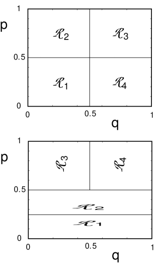
Figure 1: Partition of the unit square into four subregions, $\mathcal{R}_{1}$ through $\mathcal{R}_{4}$ (upper panel) and where each subregion maps after one iteration (lower panel). As shown, $\mathcal{R}_{1}$ and $\mathcal{R}_{2}$ are squeezed and stretched whereas $\mathcal{R}_{3}$ and $\mathcal{R}_{4}$ are rotated.

The region $\mathcal{R}_{4}$ is rotated uniquely into $\mathcal{R}_{3}$ on the next iteration and region $\mathcal{R}_{3}$ is rotated into $\mathcal{R}_{2}$. On the left half of the square, points in $\mathcal{R}_{2}$ and $\mathcal{R}_{1}$ are compressed by a factor two along the $p$ axis and stretched by the same factor along the $q$ axis.

The combination of rotation and stretching in the same dynamical system gives rise to the possibility of nonuniform hyperbolic motion or even non-hyperbolic motion. For the SR map defined as above with the vertical cut in the middle of the square at $q=0.5$, the motion is of the former kind. As the cut is moved to the right it ceases to be completely hyperbolic at the golden mean. In this paper we will only study the case when there are equal regions stretching and rotating, which is arguably the simplest “exactly solvable” model of nonuniform hyperbolicity in an area preserving map. It admits a Markov partition of phase space and the dynamics is one of subshift of finite type on three symbols as shown in Lakshminarayan (1993). The atoms of the partition are $A=\mathcal{R}_{1}\bigcup\mathcal{R}_{2},\,B=\mathcal{R}_{3},$ and $C=\mathcal{R}_{4}$.

The transition matrix is

$$T_{0}=\left(\begin{array}[]{ccc}1&0&1\\ 1&0&0\\ 0&1&0\end{array}\right)$$ (13)

whose $ij$ element, $t_{ij}$, is $1$ if there is a transition from $i$ to $j$ and $0$ otherwise. Here $i,j\,\in\ \{A,B,C\}$. This has only topological information. Let $p_{ij}$ be the fraction of atom $i$ in atom $j$, on one evolution of the map. This gives the transition probabilities for the 3-state Markov chain that the SR map is equivalent to. The transition probabilities are $p_{AA}=1/2,\,p_{AC}=1/2,\,p_{BA}=1,\,p_{CB}=1$, the rest being zero. The Markov matrix is then $T_{1}$ whose matrix elements are $t_{ij}p_{ij}$ while for fluctuations to be studied below the matrix $T_{2}$ whose elements are $t_{ij}p_{ij}^{2}$ is also useful. These matrices can be used to study the uniformity principle at the global as well as the local scales as is shown below. To study what happens on restriction to smaller areas whose size can be controlled, as well as to find the actual locations of the orbits, it is useful to use a binary representation given ahead. This is not a symbolic dynamics in the sense that the dynamics is no more a left shift. However the dynamics is an eventual left shift even in the binary representation and is used extensively below.

Any point in phase space can be represented as a bi-infinite binary string $p.q$ representing its position $q$ and momentum $p$. The binary string representing the first $m$ bits of the position coordinate is labeled $\gamma_{m}$. The quantity $m$ also corresponds to the number of times an orbit visits the stretching region (left half) of the square after some number of iterations. The rules for the mapping equations on the binary string are given in Lakshminarayan and Balazs (1993) and summarized here: if the most significant bit of position is a 0, the dynamics is that of a left shift. If the most significant bit is a 1, position and momentum coordinates are interchanged and in the new momentum coordinate all 0’s and 1’s are switched. For example, consider the period 3 orbit starting at $(q_{0},p_{0})=(2/3,1/3)$:

$$(2/3,1/3)\rightarrow(2/3,2/3)\rightarrow(1/3,2/3)\rightarrow(2/3,1/3).$$

The binary representations for the starting coordinates are $q=.\underline{10}$, $p=.\underline{01}$, where the underline indicates infinite repetition, and under the dynamics this point maps as

$$\underline{01}.\underline{10}\rightarrow\underline{01}.\underline{01}\rightarrow\underline{10}.\underline{10}\rightarrow\underline{01}.\underline{10}$$ (14)

while under the symbolic dynamics this orbit is $\underline{CBA}\rightarrow\underline{BAC}\rightarrow\underline{ACB}.$

Making use of the symbolic dynamics, it is possible to prove that the map contains a dense set of periodic orbits and is hence an ergodic transformation. It is also a straightforward argument to see that the positive Lyapunov exponent $\lambda_{L}$ for the SR map is

$$\lambda_{L}=\frac{1}{2}\ln 2.$$ (15)

This may be seen as follows: The unique smooth invariant density is uniform on the phase space. Therefore ergodicity implies that at a large number of iterations a typical orbit spends equal amounts of time on the left and right halves of the unit square. Since points along an orbit which are on the left half are stretched by a factor of two and points on the right half are not stretched at all, the Lyapunov exponent will be the average of $\ln 2$ and 0. The known symbolic dynamics, or binary representation, also allow the enumeration of all periodic orbits of any period as seen in Sect. III.2.

III.1 Periodic Orbits and Stability

To begin the discussion of the periodic orbits, first note that there exist two exceptional periodic orbits on the boundary of the square: a period 1 fixed point at the origin and a period 2 orbit between the points $(1,1/2)$ and $(1/2,1)$. All other orbits must pass through the interior of the rotating region $\mathcal{R}_{4}$ and it is thus sufficient to count orbits originating in $\mathcal{R}_{4}$. The orbits come in two types depending on the parameter henceforth called $j$, which is the number of changes from 0 to 1 or 1 to 0 in the binary string $\gamma_{m}$ representing the first $m$ bits of the position coordinate. If $j$ is odd, the orbit may be represented as $p.q=\underline{\gamma_{m}}.\underline{\gamma_{m}}$. If $j$ is even the orbit may be written as $p.q=\underline{\gamma_{m}\overline{\gamma}_{m}}.\underline{\gamma_{m}\overline{\gamma}_{m}}$ where $\overline{\gamma}_{m}$ denotes the complement of $\gamma_{m}$. From the rules given for the symbolic dynamics one finds the period $\tau$ of an orbit in terms of its $\gamma_{m}$ string to be

$$\tau=2j+m+2$$ (16)

where $j$ may take any integer value from 0 to $m-1$. Reference Lakshminarayan and Balazs (1993) may be consulted for more details.

It is also useful to realize that it is possible to translate from the binary to the symbolic dynamics and vice-versa. Sticking to orbits originating from $\mathcal{R}_{4}$ these are of the form $\cdots 0.1x_{2}x_{3}\cdots$. This translates by replacing every transition (which is a 0-1 or 1-0 ”bond” in the binary representation) including the initial 0.1 by $CBA$ and every other type (i.e. 0-0 and 1-1 bonds) by $AA$. Thus for example the orbit with the binary representation $\cdots 0.10100\cdots$ translates to $\cdots CBACBACBACBAAA\cdots$.

The Jacobian stability matrix for a single time step is dependent on whether the point in question is in the left or right half of the unit square. Denoting ${\bf M}_{L}$ as the stability matrix for points in the left half and ${\bf M}_{R}$ as the stability matrix for points in the right half we have, following from the definition of the map, that

$${\bf M}_{L}=\begin{pmatrix}{2}&{0}\cr{0}&{1/2}\cr\end{pmatrix},\hskip 5.69054pt{\bf M}_{R}=\begin{pmatrix}{0}&{-1}\cr{1}&{0}\cr\end{pmatrix}.$$ (17)

The stability matrix along a trajectory Eq. (2) may then be calculated explicitly as a product of the matrices Eq. (17). Since points in $\mathcal{R}_{4}$ always map to $\mathcal{R}_{3}$ on the next time step, the product ${\bf M}_{R}{\bf M}_{R}$ will always come in pairs in the full product for ${\bf M}_{\tau}$. Because this product ${\bf M}_{R}{\bf M}_{R}$ produces a diagonal matrix, $-\bf{I}$, the full product Eq. (2) contains only diagonal matrices, so it is commutative. This implies that up to a minus sign $\bf M_{\tau}$ is determined by the number of times an orbit visits the left half of the unit square, and the parity is determined by whether $j$ is even or odd. Putting all of this together gives the period $\tau$ Jacobian stability matrix of a particular periodic orbit as

$${\bf M}_{\tau}=\begin{pmatrix}{2^{m}(-1)^{j+1}}&{0}\cr{0}&{2^{-m}(-1)^{j+1}}\cr\end{pmatrix}$$ (18)

with eigenvalues

$$|\Lambda_{c}| =2^{-m},\hskip 11.38109pt\text{contracting}$$

$$|\Lambda_{e}| =2^{m},\hskip 11.38109pt\text{expanding}.$$ (19)

The explicit form of the inverse determinant that arises in semiclassical calculations is

$$\frac{1}{\left|{\rm Det}({\bf M}_{\tau}-{\bf 1})\right|}=\left\{{\begin{array}[]{*{20}c}{(2^{m}+2^{-m}-2)^{-1}{\text{, j odd}}}\\ {(2^{m}+2^{-m}+2)^{-1},{\text{ j even}}}\\ \end{array}}\right.$$ (20)

which may be written as with a $\pm$ for notational convenience, knowing that the sign in front of the 2 is determined by the parity of $j$. Since the main interest is in asymptotic calculations (large $\tau$) it is sufficient to keep the first two terms in the binomial expansion

$$(2^{m}+2^{-m}\pm 2)^{-1}\approx 2^{-m}-(-1)^{j}2^{-2m+1}+\cdots$$ (21)

It is shown in Sect. IV.1 that actually only the first term in the expansion is necessary to investigate certain asymptotic fluctuation properties, leaving the approximation

$$\frac{1}{\left|{\rm Det}({\bf M}_{\tau}-{\bf 1})\right|}\simeq 2^{-m}$$ (22)

Thus, for large period, to leading order $\left|{\rm Det}({\bf M}_{\tau}-{\bf 1})\right|^{-1}$ coincides with the contracting stability eigenvalue $|\Lambda_{c}|$ of the stability matrix. A final note, although the determinant is the quantity which arises in semiclassical theory, some of the classical dynamical systems literature defines the uniformity principle with respect to the inverse of the stretching exponential Ott (2002), in which case the correction term of Eq. (21) is not relevant.

III.2 Enumerating the periodic points

It is quite valuable to be able to count the periodic points of fixed period in a given subregion of the unit square. To do so we proceed as follows: divide the unit square into a grid of boxes of area $2^{-k}\times 2^{-k}$ , whose lower left corners are specified by $q=.x_{1}x_{2}...x_{k}$ and $p=.y_{1}y_{2}...y_{k}$. This is a binary expansion, so each $x_{i}$ and $y_{i}$ is either 0 or 1. This is a total of $4^{k}$ boxes. Membership of an orbit in a box with a specified lower left corner is simply that the orbit has the same first $k$ bits for $p$ and $q$ in its binary representation as the lower left corner, and arbitrary bits beyond the $k$th. To start, consider boxes in the lower right subsquare $\mathcal{R}_{4}$. The same counting results will hold for regions $\mathcal{R}_{3}$ and $\mathcal{R}_{2}$ since these are merely rotations of $\mathcal{R}_{4}$. The slightly more detailed counting arguments for region $\mathcal{R}_{1}$ can be found in Appendix A.

As in Sect. III.1 the periodic points are written either in the form $\underline{\gamma_{m}}.\underline{\gamma_{m}}$ or $\underline{\gamma_{m}\overline{\gamma}_{m}}.\underline{\gamma_{m}\overline{\gamma}_{m}}$, the former if $j$, the number of 0-1 or 1-0 transitions in $\gamma_{m}$, is odd, and the latter if $j$ is even. The requirement on the string $\gamma_{m}$ for a point to be in $\mathcal{R}_{4}$ is that the first bit is 1. If the last bit is 0, then the first form represents a point in $\mathcal{R}_{4}$, and if the last bit is 1, then it is the second form that is a point in $\mathcal{R}_{4}$. In either case, $m$ is related to the period $\tau$ by Eq. (16). Note that $j\leq m-1$, so $j\leq\tau-2j-3$ and $3j\leq\tau-3$, so that $j$ is at most $\lfloor(\tau/3)\rfloor-1$ where $\lfloor\cdots\rfloor$ denotes the floor function. The first step is to count how many $\tau$-periodic points with a fixed value of $j$ there are in the box whose corner is specified by $q=.1x_{2}...x_{k}$ and $p=.0y_{2}...y_{k}$ (note the 1 and the 0 are forced because the point must lie in $\mathcal{R}_{4}$). This point is also represented by combining the binary expansions into one expression $y_{k}y_{k-1}...y_{2}0.1x_{2}...x_{k}$, and similarly for other points.

For a $\tau$-periodic point of the first form, $\gamma_{m}$ must look like $1x_{2}...x_{k}w_{1}...w_{i}y_{k}...y_{2}0$ for some $i,k$ with the restriction $i=\tau-2j-2k-2$ and the total number of transitions in this string is $j$. If the periodic point is of the second form, then $\gamma_{m}=1x_{2}...x_{k}w_{1}...w_{i}\bar{y}_{k}...\bar{y}_{2}1$.

Let $s$ equal the number of 0-1 or 1-0 transitions in $1x_{2}...x_{k}$ plus the number of 0-1 or 1-0 transitions in $0y_{2}...y_{k}$. That is, $s$ is the total number of changes for the lower left corner point of the box. If $s$ and $j$ are both odd, a periodic point would be of the first form, and $\gamma_{m}=1x_{2}...x_{k}w_{1}...w_{i}y_{k}...y_{2}0$. There are $s$ transitions from 1 to $x_{k}$ and from $y_{k}$ to 0 combined, so there must be $j-s$ transitions in the $i+1$ possible places in $x_{k}w_{1}...w_{i}y_{k}$. So there are $\left({\begin{array}[]{*{20}c}{i+1}\\ {j-s}\\ \end{array}}\right)=\left({\begin{array}[]{*{20}c}{\tau-2j-2k-1}\\ {j-s}\\ \end{array}}\right)$ ways to do this. In the other cases in which $j$ and $s$ may be either even or odd, the same result holds and thus we have that for each possible value of $j$, the number of $\tau$-periodic points in a $2^{-k}$ $\times$ $2^{-k}$ box in $\mathcal{R}_{4}$ with corner value specified by $s$ is $\left({\begin{array}[]{*{20}c}{\tau-2j-2k-1}\\ {j-s}\\ \end{array}}\right)$. The smallest possible value of $j$ is $s$, which occurs when all the $w$’s are the same as $x_{k}$, and the maximum attainable value of $j$ is $\lfloor(\tau-2k+s-1)/3\rfloor$. In addition, for a given value of $s$, there are $\left({\begin{array}[]{*{20}c}{2k-2}\\ s\\ \end{array}}\right)$ possible $2^{-k}$ $\times$ $2^{-k}$ boxes with $s$ the number of transitions in the first $k$ $p$-bits plus transitions in the first $k$ $q$-bits of the corner point.

To summarize, the counting just given is for $\tau$-periodic points in a binary grid of boxes within $\mathcal{R}_{4}$, $\mathcal{R}_{3}$, and $\mathcal{R}_{2}$ where $k$ is the number of bits specifying a box side, and $s$ is the number of transitions in the $k$ bits of the $q$-coordinate of the corner of the box plus the number of transitions in the $k$ bits of the $p$-coordinate of the corner point. The index $j$ ranges from $s$ to $\lfloor(\tau-2k+s-1)/3\rfloor$ and for a given $j$ the number of periodic points with that value of $j$ is given by $\left({\begin{array}[]{*{20}c}{\tau-2j-2k-1}\\ {j-s}\\ \end{array}}\right)$, so the total number of period-$\tau$ points in this box is

$$N_{\tau}(s,k)=\sum_{j=s}^{\lfloor(\tau-2k+s-1)/3\rfloor}{\begin{pmatrix}{\tau-2j-2k-1}\cr{j-s}\cr\end{pmatrix}}.$$ (23)

Note that for fixed period and box size, the statistics of the periodic points within a box are determined entirely by the value $s$ of its corner point. Any two boxes with the same value of $s$ will have exactly the same distribution, and for each $s$ there are $\left({\begin{array}[]{*{20}c}{2k-2}\\ s\\ \end{array}}\right)$ such boxes. Thus, the Hannay-Ozorio sum, Eq. (1), over all periodic points within a binary box in $\mathcal{R}_{4}$, $\mathcal{R}_{3}$, or $\mathcal{R}_{2}$ is

$$F_{\tau}(s,k)=\sum_{j=s}^{\lfloor(\tau-2k+s-1)/3\rfloor} \begin{pmatrix}{\tau-2j-2k-1}\cr{j-s}\cr\end{pmatrix}$$

$$\times\frac{1}{\left|{\rm Det}({\bf M}_{\tau}-{\bf 1})\right|}$$ (24)

and the global form of Eq. (1) (excluding $\mathcal{R}_{1}$) by summing over all boxes in $\mathcal{R}_{4}$, $\mathcal{R}_{3}$, and $\mathcal{R}_{2}$ gives

$$F_{\tau}=3\sum_{s=0}^{2k-2}\begin{pmatrix}{2k-2}\cr{s}\cr\end{pmatrix}F_{\tau}(s,k).$$ (25)

The relation of the inverse determinant to the period and the symbolic representation of an orbit is, from Eq. (22) and Eq. (16), given by

$$\frac{1}{\left|{\rm Det}({\bf M}_{\tau}-{\bf 1})\right|}\simeq 2^{-\tau+2j+2}$$ (26)

which provides an explicit summable expression for looking at fluctuations in the uniformity principle.

The counting arguments for the subsquare $\mathcal{R}_{1}$ are slightly different, but similar in character, to those presented here and the details are given in Appendix A. In fact, the resulting equations are quite close to the ones given in this section.

Figure 2 shows a plot of all periodic points in the unit square at $\tau=24$ and $28$. This visualization of the structure of the periodic points is interesting in its own right, as the points appear to have a fractal-like structure to them. In fact the checkered pattern created mimics the stable and unstable manifolds of the map.

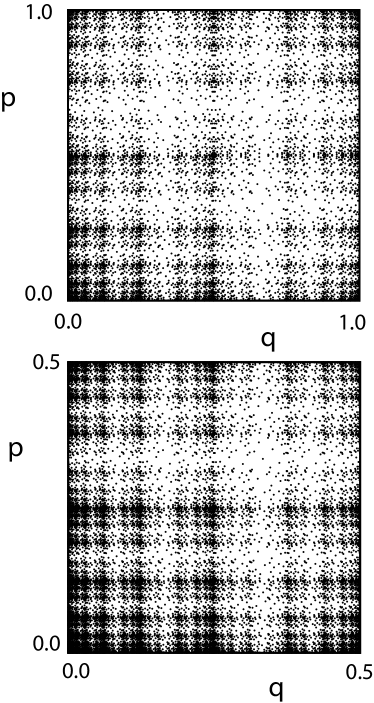
Figure 2: Fixed points of the time $\tau$ iterated map. The upper square is the plot for $\tau$ = 24 and the lower square is the $R1$ region for $\tau$ = 28. The density of fixed points at $\tau=28$ is roughly 4.6 times that of $\tau=24$. Below, expanding $R1$ renders the lower plot’s fixed point density similar to the upper plot. The similarity of the expanded $R1$ fixed point’s structure to the full phase space at an earlier time illustrates the fractal-like structure mentioned in the text.

The symbolic dynamics and the Markov matrices can also be used to find the number of periodic orbits as well as to study the uniformity principle. Since the SR map is simple enough to permit both a combinatorial approach as well as a symbolic dynamics one, it is useful to present both. Given a periodic point of the first type in $\mathcal{R}_{4}$ whose $\gamma_{m}$ string has a binary representation $1x_{2}x_{3}\cdots w_{1}w_{2}\cdots w_{i}y_{k}\cdots y_{2}0$, this translates into an orbit which is a repetition of symbol strings of length $\tau=2j+2k+i+2$. Of these $3(s+1)+[2(k-1)-s]=2s+2k+1$ are utilized to specify the fixed corner point. Thus there are $n=\tau-(2s+2k+1)$ number of possible “free” symbols, say $S_{1},\ldots S_{n}$. A little thought shows that the free symbol string has to end with $A$, that is $S_{n}=A$, and has to be prefixed by an $A$. Thus it can be either of the form $CBA\cdots A$ or $A\cdots A$. In both these cases the number of periodic points is then given by

$$N_{\tau}(s,k)=\sum_{S_{i}}(T_{0})_{AS_{1}}(T_{0})_{S_{1}S_{2}}\cdots(T_{0})_{S_{n-1}A},$$ (27)

or

$$N_{\tau}(s,k)=\left(T_{0}^{\tau-2k-2s-1}\right)_{AA}.$$ (28)

Recall that $T_{0}$ is the transition matrix in Eq. (13). Thus the combinatorial problem can be reduced to that of finding powers of a matrix. From this point the mathematical complexity is comparable as both lead to the analysis of cubic equations; see Appendix B for the combinatorial case.

The uniformity principle sum for the local area can also be written compactly in terms of a matrix power, this time the Markov matrix $T_{1}$. A similar reasoning as above leads to

$$F_{\tau}(s,k)=\dfrac{1}{2^{2k-1}}\left(T_{1}^{\tau-2k-2s-1}\right)_{AA}.$$ (29)

Here however, the approximation in Eq. (26) is already used, as otherwise such a compact formula is not possible. Note that with this approximation the global (over the whole phase space) uniformity principle sum is simply the trace of the power of the Markov matrix. That is

$$F_{\tau}=\mbox{Tr}(T_{1}^{\tau}).$$ (30)

This follows from the fact that the entries in the stochastic matrix $T_{1}$ are precisely the multipliers which are either $1/2$ or $1$. That the stochastic matrix has necessarily an eigenvalue 1, and therefore $F_{\tau}\rightarrow 1$ as $\tau\rightarrow\infty$ is an alternative formulation of the uniformity principle. The other eigenvalues of $T_{1}$ whose eigenvalues are less than 1 in modulus determine both the rate of decay of correlations as well as approach to uniformity of the periodic orbits. We will expand on this below shortly. Almost all of the analysis below follows the consequences of the binary representation and the combinatorial approach as detailed statistics is more transparently done this way.

IV Statistical Results

The results of the previous section and Appendix B can be used to evaluate sum rule fluctuations. Consider the local density of the inverse determinant $\left|{\rm Det}({\bf M}_{\tau}-{\bf 1})\right|^{-1}$, which occurs as the natural weighting for periodic orbits in many semiclassical expressions. The first goal is to derive an asymptotic formula for its variance. This analysis leads naturally to discussing the density and convergence of the remaining component $\tilde{F}_{\tau}(s,k)$ of the Hannay-Ozorio sum rule introduced in Sect. II.2.2. We give an analytic expression for $\tilde{F}_{\tau}(s,k)$ and compute its variance, as well as local and global boundaries of convergence for the sum rule.

IV.1 Local distribution of the inverse determinant

Consider the regions $\mathcal{R}_{4}$, $\mathcal{R}_{3}$, and $\mathcal{R}_{2}$ (see Fig. 1) of the unit square whose density of periodic orbits is described in Sect. III.2. As before, the (similar) discussion for the region $\mathcal{R}_{1}$ is left to Appendix A. There is a range of values taken by $\left|{\rm Det}({\bf M}_{\tau}-{\bf 1})\right|^{-1}$ within a local patch of phase space, as described in Sect. III.2. It was shown that the number of period $\tau$ fixed points with a fixed value of the determinant specified by $j$ in a box with parameters $s$ and $k$ is given by $\begin{pmatrix}{\tau-2j-2k-1}\cr{j-s}\cr\end{pmatrix}$ where $j\geq s$. For large period the combinatorial as a function of allowed values of $j$ (which can be thought of as a probability density for various stability determinant values of fixed points in the box) is approximately normally distributed (see Appendix B) with an exact mean given by Eq. (149), but written approximately here as

$$\mu\simeq\frac{{\tau-2s-2k-1}}{{5.148}}\,\,\,+\,\,\,s\,\,-0.162.$$ (31)

Recall from Eq. (26) that at period $\tau$ the inverse determinant may take on the values $2^{-\tau+2j+2}$ as $j$ ranges from $s$ to $\lfloor(\tau-2k+s-1)/3\rfloor$. So in fact, for the discussion of $\left|{\rm Det}({\bf M}_{\tau}-{\bf 1})\right|^{-1}$, the sum rule $F_{\tau}(s,k)$ is over terms of the form $\begin{pmatrix}{\tau-2j-2k-1}\cr{j-s}\cr\end{pmatrix}4^{j}$. It turns out that the density for these terms is normal as before for the $t=0$ case; note, oddly enough, that does not imply that the density for finding a particular value of the inverse determinant is lognormal as the convergence with $\tau-2j-2k-1\rightarrow\infty$ to normal is too slow.

Consider the density $g(i,t)=\begin{pmatrix}{n-2i}\cr{i}\cr\end{pmatrix}e^{ti}$ as a function of $i$ for a given $t$, where as in Appendix B, $e^{t}=\alpha$. Using Stirling’s formula to approximate $g(i,t)$, and calculus, one finds that the maximum value of $g(i,t)$ occurs at the value $i_{0}$ of $i$ given by

$$i_{0}\approx n\frac{\beta_{1}(t)-1}{3\beta_{1}(t)-2}$$ (32)

where $\beta_{1}(t)$ is the real root of the cubic equation $\beta^{3}-\beta^{2}-e^{t}=0$. Interestingly this same cubic equation arises here for a different problem from the one considered in Appendix B. This method does not give the exact transient terms as the recurrence method of Appendix B does, but the same structure exists and near the maximum at $i_{0}$, $g(i,t)$ is approximated continuously as a Gaussian with width on the order of $\sqrt{n}$ and so the values of $i$ which contribute to the sum are sharply peaked around the maximum. Specifically,

$$g(i,t) =\left({\begin{array}[]{*{20}c}{n-2i}\\ i\\ \end{array}}\right)e^{ti}$$ (35)

$$\simeq\frac{\beta_{1}^{n+1}}{{3\beta_{1}-2}}\frac{1}{{\sqrt{2\pi\sigma^{2}_{i}}}}e^{-\,(i-i_{0})^{2}/(2\sigma^{2}_{i})}$$ (36)

where $\sigma^{2}_{i}=n\frac{{\beta_{1}(\beta_{1}-1)}}{{(3\beta_{1}-2)^{3}}}$.

For the quantity $\left|{\rm Det}({\bf M}_{\tau}-{\bf 1})\right|^{-1}$, for which $e^{t}=4$, $\beta_{1}=2$ and so the mean of $g(i,t)$ occurs at $i_{0}=n/4$, even though the mean $\mu(n)$ (for the unweighted combinatorial) occurs at about $n/5.148$. As $n\rightarrow\infty$, the two densities tend toward a vanishing overlap since the difference in the means grows faster than the widths. In considering values taken by the inverse determinant, only those periodic points with transition number $j$ which occur near

$$j_{0}=\frac{\tau-2s-2k-1}{4}+s$$ (37)

contribute to the sum $F_{\tau}(s,k)$, in spite of the fact that there is a vanishing relative fraction of fixed points associated with this value of $j$, as most points have a value of $j$ near $(\tau-2s-2k-1)/5.148+s-0.162$.

IV.2 Important Moments

We give here explicit expressions for some of the quantities of interest related to the inverse determinant and the SR map, using the results from the methods of Appendix B. First consider the number of period $\tau$ fixed points within a binary box specified by $s$ and $k$. The number $N_{\tau}(s,k)$ is given by Eq. (23), which is a special case of the sum formula $S(n,\alpha)$ from Appendix B with $\alpha=1$ and $n=\tau-2k-2s-1$. The form of the solution is therefore specified by Eq. (146), with appropriate values for the constants. The topological entropy is given by $h_{T}=\ln\beta_{1}(0)$, and thus

$$N_{\tau}(s,k)=c_{1}e^{h_{T}n}\,+2e^{-h_{T}n/2}\left[a\cos(n\theta)-b\sin(n\theta)\right]$$ (38)

This equation contains the finite-time correction terms to the count of fixed points of a binary box, which cannot be given by specifying the entropy alone. If $\tau$ is large, the leading term $c_{1}e^{h_{T}n}$ dominates and may be used for asymptotic calculations.

The moments for the inverse determinant (which are different from the moments involved in the sum rule fluctuations, ahead) may be computed by averaging over powers of $\left|{\rm Det}({\bf M}_{\tau}-{\bf 1})\right|^{-1}$. The most important case is the mean, which corresponds to $F_{\tau}(s,k)$, and gives an explicit finite-time correction term to the (infinite time) prediction of the uniformity principle. It is also an ingredient of other sum rule moments.

From Eq. (24) and Eq. (26), the local form of the sum of the inverse determinant over all fixed points within a box reads

$$F_{\tau}(s,k)=\sum\limits_{j=s}^{\left\lfloor{(\tau-2k+s-1)/3}\right\rfloor}{\left({\begin{array}[]{*{20}c}{\tau-2j-2k-1}\\ {j-s}\\ \end{array}}\right)}2^{-\tau+2j+2}$$ (39)

which is predicted by the Hannay-Ozorio sum rule to asymptotically approach the area of the box, $4^{-k}$. A slight change of variables puts the sum in the generic form, Eq. (126), with $\alpha=4$ and $n=\tau-2k-2s-1$. The solution is thus again of the form of Eq. (146), where the real root $\beta_{1}$ of the cubic is exactly 2. After some algebraic manipulation, it is seen that $F_{\tau}(s,k)$ may be written in a form which displays both its exponential dependence on the period as well as its relation to the phase space area as

$$F_{\tau}(s,k)=4^{-k}+e^{-\lambda_{L}\tau}2^{s-k+5/2}[a\cos(n\theta)-b\sin(n\theta)]$$ (40)

where $\lambda_{L}$ is the real part of the leading Pollicot-Ruelle resonance (here also equal to the positive Lyapunov exponent) whose value is given in Eq. (15). The numerical values of the constants $a$, $b$, and $\theta$ may be calulated using the formulas of Appendix. B. Subtracting the Hannay-Ozorio term leaves the oscillating part with time of the sum rule as

$$\tilde{F}_{\tau}(s,k)=e^{-\lambda_{L}\tau}2^{s-k+5/2}[a\cos(n\theta)-b\sin(n\theta)].$$ (41)

By factoring out the time dependence, it turns out that the rate of convergence towards uniformity with increasing period is exponential, as expected. It is clear from the discussion based on symbolic dynamics and Eq. (29) that the rate is governed by the eigenvalues of a Markov matrix if it exists or generally by the Pollicott-Ruelle resonances. In the case of the SR map, the modulus of the eigenvalues of the Markov matrix, which are the resonances, have modulus equal to $1/\sqrt{2}$, which is $e^{-\lambda_{L}}$. It is well-known that the Pollicott-Ruelle resonances are generically not related to the Lyapunov exponents and therefore the equality for the SR map must be considered a coincidence. The close connections between mixing and uniformity principle makes the emergence of the Pollicott-Ruelle resonances as governing the rate of convergence to uniformity much more natural.

It is also interesting to consider the convergence boundary as mentioned in Sect. II.2.1. This amounts to determining the box size (phase space volume) for a given period and location in phase space at which the size of the correction term $\tilde{F}_{\tau}(s,k)$ is just the same order of magnitude as the local area itself. In particular, from Eq. (41), if $2^{-\tau/2+s-k+5/2}=4^{-k}$ then $k=\tau/2-s-5/2$ and the volume at the convergence boundary is

$$\mathcal{V}(s;\tau)=2^{-\tau+2s+5}.$$ (42)

In this way, the local sum rule fluctuations are equally as important as the mean, and hence to any results which invoke a sum rule on that local scale at that time. Given that $s$ varies in the domain $0\leq s\leq 2k-2$ or in terms of $\tau$, $0\leq 3s\leq 2\tau-7$, the convergence boundary varies greatly from one location to another in the phase space, i.e. $2^{-\tau}\leq\mathcal{V}(s;\tau)\leq 2^{-\tau/3}$. Although the local convergence boundary vanishes everywhere as $\tau\rightarrow\infty$, its relative variation tends to infinity. The relatively larger boundaries are precisely linked to locally greater inverse determinant variation just ahead.

In Eq. (21), the leading correction term to the inverse determinant was given, but up to this point not included in the calculations. It is important to know if this error is subdominant relative to the fluctuating component just calculated. If the second expansion term is kept, this leads to a sum denoted $\tilde{B}_{\tau}(s,k)$ of the form

$$\tilde{B}_{\tau}(s,k)=\sum\limits_{j=s}^{\left\lfloor{(\tau-2k+s-1)/3}\right\rfloor} {\left({\begin{array}[]{*{20}c}{\tau-2j-2k-1}\\ {j-s}\\ \end{array}}\right)}$$ (45)

$$\times 2^{-2\tau+5}(-16)^{j}$$ (46)

which once again is in the form of the sum discussed in Appendix B with $\alpha=-16$ and $n=\tau-2s-2k-1$.

In fact, more properly, the two most dominant corrections to the local sum rule are

$$F_{\tau}(s,k)=4^{-k}+\tilde{F}_{\tau}(s,k)-\tilde{B}_{\tau}(s,k)$$ (47)

We know that the first correction term is governed by the Pollicott-Ruelle resonances, but the second term is something else. A priori, it is not obvious which of these two correction terms dominates for large period. Extracting only the exponential dependence on $\tau$ gives $\tilde{F}_{\tau}(s,k)\propto e^{-\lambda_{L}\tau}\approx(0.71)^{\tau}$. For $\tilde{B}_{\tau}(s,k)$, because $\alpha<0$, the dominant fluctuation term comes from the oscillatory $(\alpha/\beta)^{n/2}$, which is approximately $\tilde{B}_{\tau}(s,k)\approx(0.67)^{\tau}$. In this case, the first correction term eventually dominates over the second, and using the approximation of Eq. (26) is justified. Had the situation turned out the opposite way, then the correction term would not have been a Pollicott-Ruelle resonance; we are not aware of an argument suggesting that this could not have happened and thus both sources of corrections must be considered in other cases.

Before continuing with the spatial fluctuations in the sum rule itself, consider the variation of the individual inverse determinants contributing to each sum. They vary wildly from one fixed point to the next and there is greater variation in some regions as opposed to others. This gives an $s$-dependence to their variation within any single box. This can be seen by computing the variance. The sum of squares of the inverse determinant, $Q_{\tau}(s,k)$, is given by

$$Q_{\tau}(s,k) =\sum_{f.p.}\frac{1}{\left|{\rm Det}({\bf M}_{\tau}-{\bf 1})\right|^{2}}$$

$$=\sum\limits_{j=s}^{\left\lfloor{(\tau-2k+s-1)/3}\right\rfloor}{\left({\begin{array}[]{*{20}c}{\tau-2j-2k-1}\\ {j-s}\\ \end{array}}\right)}2^{-2\tau+4j+4}$$ (50)

This is a sum of the form of Eq. (126) with $\alpha=16$ and $n=\tau-2k-2s-1$. Keeping only the leading term in Eq. (146), the solution is

$$Q_{\tau}(s,k)=4^{-\tau+2s+2}c_{1Q}\beta_{1Q}^{\tau-2k-2s-1}$$ (51)

where $\beta_{1Q}$, the real root of the cubic polynomial for $\alpha=16$, is approximately 2.901 and $c_{1Q}\approx 0.433$. The subscripts on the numerical constant $c$ and $\beta$ are used here to make it clear that these refer to the case $Q$, for which $\alpha=16$. The same result can also be derived from the symbolic dynamics as

$$Q_{\tau}(s,k)=\dfrac{1}{4^{2k-1}}\left(T_{2}^{\tau-2k-2s-1}\right)_{AA}.$$ (52)

In the notation of Eq. (6), the variance of the inverse determinants within a given box is $\sigma^{2}(e^{\lambda\tau})={\cal M}_{-2}(e^{\lambda\tau},s,k)-{\cal M}_{-1}(e^{\lambda\tau},s,k)^{2}$ and

$$\sigma^{2}(e^{\lambda\tau},s,k)=\frac{Q_{\tau}}{N_{\tau}}-\left(\frac{4^{-k}}{N_{\tau}}\right)^{2}\approx\frac{Q_{\tau}N_{\tau}-2^{-4k}}{N_{\tau}^{2}}$$ (53)

where the leading order of the mean is sufficient. The product $Q_{\tau}N_{\tau}$ depends on $\tau$ by a factor $(e^{h_{T}}\beta_{1Q}/4)^{\tau}$, which is greater than unity. Thus, this term diverges as $\tau\rightarrow\infty$. Asymptotically the local variance is just $Q_{\tau}/N_{\tau}$, or

$$\sigma^{2}(e^{\lambda\tau},s,k)\longrightarrow\frac{16c_{1Q}}{c_{1N}}\left({\frac{{\beta_{1Q}}}{{4e^{h_{T}}}}}\right)^{\tau-2s}\left({\frac{{\beta_{1Q}}}{{e^{h_{T}}}}}\right)^{-2k-1}$$ (54)

which shows asymptotically how the variance varies with $s$, a local characteristic of a particular region of phase space (box). Here $\beta_{1Q}/e^{h_{T}}$ is about 1.98 and $\beta_{1Q}/4e^{h_{T}}$ is about 0.495. When the analogous details are worked out for boxes in the region $\mathcal{R}_{1}$, the variance differs only by a constant factor of $16\left(\frac{\beta_{1Q}}{e^{h_{T}}}\right)^{2}$.

Note that boxes whose lower-left corner has a small number of transitions (small $s$) have smaller variances, as well as more $\tau$-periodic points, than boxes with large $s$. Precisely as found for the local convergence boundaries, the variation of $s$ for moderately large $k$ leads to an enormous difference in the variations within different boxes of the same size. Although, the variances vanish in the limit of $\tau\rightarrow\infty$, the ratios of the variances from one box to another another increase indefinitely as the box size shrinks.

IV.3 Sum rule fluctuations

Next the global variance of the local sum rule $F_{\tau}(s,k)$ is considered due to spatial variation. First we comment on the form of the density of $F_{\tau}(s,k)$. Recall that with the method of subdividing the phase space into a grid of binary boxes, the value of $F_{\tau}(s,k)$ locally within a box is specified by a parameter $s$ which counts the number of 0 to 1 changes in the binary representation of the lower left corner of the box (see Sect. III.2). Thus, $\tilde{F}_{\tau}(s,k)$ depends exponentially on $s$, Eq. (41). Furthermore, the number of boxes throughout a quarter region of the unit phase space square with a given value of $s$ is $\begin{pmatrix}{2k-2}\cr{s}\cr\end{pmatrix}$, as $s$ ranges from 0 to $2k-2$. Thus, the density of the logarithm of $\tilde{F}_{\tau}(s,k)$ follows a binomial centered at $k-1$. As with the inverse determinant, the distribution of $\tilde{F}_{\tau}(s,k)$ is described by the product of an exponential function (of $s$, here) and a combinatorial coefficient that is approximately normal. A qualitatively similar behavior to the discussion of Sect. IV.1 arises in describing the density of values taken by the sum formula $\tilde{F}_{\tau}(s,k)$.

The variance of $\tilde{F}_{\tau}(s,k)$ is the average square deviation from the mean summing over all boxes and dividing by their total number, $4^{k}$. This is essentially the second moment defined in Sect. II.2.2

$${\cal M}_{2}(\tilde{F}_{\tau},k)=\frac{1}{4^{k}}\sum_{s=0}^{2k-2}\left(\begin{array}[]{c}2k-2\\ s\\ \end{array}\right)\tilde{F}_{\tau}(s,k)^{2}$$ (55)

For calculational convenience, Eq. (41) is rewritten in the form

$$\tilde{F}_{\tau}(s,k)=Ae^{\gamma s}+(Ae^{\gamma s})^{*}$$ (56)

where $\gamma=\ln{2}-2\theta i$ and $A=c_{2}2^{-\tau/2-k+3/2}e^{i\theta(\tau-2k-1)}$. Recall that the constants $c_{2}$ and $\theta$ arise from the solutions of the sum formula in Appendix B, in this case for $\alpha=4$. This result holds for the regions $\mathcal{R}_{4}$, $\mathcal{R}_{3}$, and $\mathcal{R}_{2}$ of the unit square. For $\mathcal{R}_{1}$, the expression used for $F_{\tau}(s,k)$ differ only by a constant factor, as shown in Appendix A, and this factor is accounted for below in giving the variance over the entire unit square.

For large $k$, it is possible to find a simplified asymptotic expression for the variance. Let $c_{2}=|c_{2}|e^{i\zeta}$ and $\eta=\theta(\tau-2k-1)+\zeta$ giving

$$[Ae^{\gamma s}+(Ae^{\gamma s})^{*}]^{2}=|c_{2}|^{2}2^{-\tau-2k+3}[2^{2s+1}+2\text{Re}(e^{2i\eta}e^{2\gamma s})].$$ (57)

The expression for the variance becomes

$${\cal M}_{2}(\tilde{F}_{\tau},k)= \hskip 2.84526pt4^{-k}|c_{2}|^{2}2^{-\tau-2k+4}\left[\sum_{s=0}^{2k-2}{\left({\begin{array}[]{*{20}c}{2k-2}\\ s\\ \end{array}}\right)4^{s}}\right.$$ (60)

$$\hskip 14.22636pt\left.+\text{Re}(e^{2i\eta}\sum_{s=0}^{2k-2}{\left({\begin{array}[]{*{20}c}{2k-2}\\ s\\ \end{array}}\right)e^{2\gamma s}})\right].$$ (63)

Recalling the binomial theorem, each term above may be summed explicitly to give

$${\cal M}_{2}(\tilde{F}_{\tau},k)= |c_{2}|^{2}2^{-\tau}16^{-k+1}\left[5^{2k-2}\right.$$

$$\hskip 14.22636pt\left.+\text{Re}\left(e^{2i\eta}\left[1+e^{2\gamma}\right]^{2k-2}\right)\right].$$ (64)

Letting $1+e^{2\gamma}=1+4e^{-i4\theta}=\rho e^{i\omega}$ where $\rho^{2}=17+8\cos(4\theta)$ gives

$${\cal M}_{2}(\tilde{F}_{\tau},k) =|c_{2}|^{2}2^{-\tau-4k+4}\left[5^{2k-2}+\rho^{2}\cos(2\eta+2\omega[k-1])\right]$$

$$=|c_{2}|^{2}2^{-\tau}\left(\frac{25}{16}\right)^{k-1}$$

$$\hskip 11.38109pt\times\left[1+\left(\frac{\rho^{2}}{25}\right)^{k-1}\cos(2\eta+2\omega[k-1])\right].$$ (65)

Since $4\theta$ is not a multiple of $2\pi$, $\cos(4\theta)$ is less than unity and so is $\rho^{2}/25$. Thus, the oscillatory terms are subdominant as $k$ increases. For large $k$, or small local volume, the expression for the variance in each of regions $\mathcal{R}_{4}$, $\mathcal{R}_{3}$, and $\mathcal{R}_{2}$ becomes:

$${\cal M}_{2}(\tilde{F}_{\tau},k)\simeq(3/4)|c_{2}|^{2}e^{-2\lambda_{L}\tau}(5/4)^{2k-2}.$$ (66)

For the region $\mathcal{R}_{1}$ the same equation for $\tilde{F}_{\tau}(s,k)$ as Eq. (56) applies except that the coefficient $A$ is replaced by $A^{\prime}=c_{2}2^{-\tau/2-k+1/2}e^{i\theta(\tau-2k+1)}$. From this it follows that the contribution to the variance from the region $\mathcal{R}_{1}$ is simply one fourth the value for $\mathcal{R}_{4}$, $\mathcal{R}_{3}$, or $\mathcal{R}_{2}$. The asymptotic formula for the variance of $F_{\tau}$ taken over the entire unit square is

$${\cal M}_{2}(\tilde{F}_{\tau},k)\simeq\frac{13}{16}|c_{2}|^{2}e^{-2\lambda_{L}\tau}\left(\frac{5}{4}\right)^{2k-2}.$$ (67)

The variance thus decreases exponentially with time, again governed by the Pollicott-Ruelle resonance. It also increases with the decreasing local volumes. This gives a global convergence boundary for the sum rule on which the variance over the entire phase space remains a constant (rather than vanishing). From Eq. (67) this would be given approximately by $k=\frac{\lambda_{L}\tau}{\ln{5/4}}$, and

$$\mathcal{V}(\tau)=2^{-\tau\ln{2}/\ln{5/4}}\approx 2^{-3.1\tau}.$$ (68)

V Concluding Remarks

The convergences and fluctuations of classical sum rules are interesting in a multitude of ways. Although, their corrections may be exponentially suppressed with increasing time, the individual contributions can have a diverging variance themselves. Another interesting feature of local sum rules, as shown herein, is that certain fluctuations can be surprisingly large as the location of phase space is varied. Correction terms may be related to known properties of the system in more general dynamical systems, such as the topological entropy, the Pollicott-Ruelle resonances, or the Lyapunov exponent depending on the precise sum rule of interest. It would appear that a fluctuation quantity, which depends sensitively on some higher power of the stability determinant, if such a quantity exists, may be more likely to reflect the kinds of fluctuations that have been described here on a theoretical basis for the SR map. The results, however, may be suggestive of the type of behavior one might expect in a regime where sum rule fluctuations could arise. The asymptotic form of several different fluctuation measures derived for the Hannay-Ozorio sum, as well as their time and length scales, came from the solution of the same simple cubic polynomial. The origin of this lies in the symbolic dynamics which is a subshift of finite type on three symbols and thus there is an equivalent three state Markov chain. It may be the case that similar methods could be applied to other relatively simple systems, and that sum rule corrections could also be derived for these systems from the basis of their dynamics.

The main results for the SR map begin with the calculation of the two sources of fluctuations in the Hannay-Ozorio sum rule. The first source is governed by the dominant Pollicott-Ruelle resonances. It arises from the non-uniformity of the locations of fixed points and their non-uniform weighting by the leading behavior of their inverse stability determinants. The second source arises from the effects of next-to-leading order corrections to the inverse stability determinants. These corrections are not governed by the Pollicott-Ruelle resonances, but are also exponentially decreasing in time. The dominant correction here comes from the first source and hence the Pollicott-Ruelle resonances, however we do not currently know whether this must be the case for general chaotic dynamical systems.

It is a matter of how closely the stretching multipliers approximate the determinant in Eq. (20), and it could be that for some other chaotic system they are different enough to produce corrections that dominate the one due to the resonances, although these would still be present. In the specific case of the SR map the second term in Eq. (21), the principal correction, is an oscillating sum because the periodic orbits are reflecting hyperbolic if the number of $0-1$,$1-0$ bonds are odd. This term can be written as a trace of the power of the matrix

$$\left(\begin{array}[]{ccc}1/4&0&1/4\\ -1&0&0\\ 0&1&0\end{array}\right)$$ (69)

which is different from the $T_{2}$ matrix in that the element $(2,1)$ is $-1$ rather than $1$. This ensures that each time the orbit gets rotated, it acquires a negative sign. Alternately, for each CBA part of the symbolic string a negative sign is acquired.

The leading eigenvalue of this matrix has a modulus of $\approx 0.67$ which is smaller than the subleading eigenvalue, $\approx 0.707$, of $T_{1}$ that gives the Pollicot-Ruelle resonance. If the orbit were all direct hyperbolic then in the above matrix the $-1$ will change to $1$ and this will be same as $T_{2}$ whose leading eigenvalue is $0.725$ which is larger than $0.707$, and would have dominated the corrections. The fact that some of the orbits are reflecting hyperbolic seems to have been crucial to lower the contribution from corrections that come from the fact that a $\mbox{\rm det}\,(J-I)$ is present instead of just the multipliers.

However if the sum rule is weighted by (the inverse) of the largest eigenvalue of the stability matrix, the Pollicott-Ruelle resonances will govern the corrections to the sum rule, especially if there is a finite symbolic dynamics description of the system. The relevance of Markov and related matrices ($T_{0},T_{1},T_{2},\ldots$) for the calculation of the fluctuations indicate possible connections with the Thermodynamic Formalism especially as applied to finite Markov processes Gaspard (1998).

A second result shows how the relative local variations of the inverse determinants varies infinitely broadly at long times. Finally, the relative variation of the sum rule applied locally also has an infinite width while maintaining an exponential convergence rate for fixed phase space volume. We gave convergence boundaries that show how small a local volume may be considered for a given time of propagation if one expects convergence to the asymptotic sum rule result. Again, the relative size of a converged local volume depended on location and varied infinitely broadly while maintaining exponential convergence with time at fixed volume

It would be extremely interesting to investigate other sum rules, especially those that connect to quantum fluctuation properties of eigenfunctions and transport. The various localizing effects giving rise to eigenfunction scarring Heller (1984), localization manifestations of time scales introduced by transport barriers Bohigas et al. (1993), and interaction effects linked to Friedel oscillations Tomsovic et al. (2008); Ullmo et al. (2009) give a few interesting directions for further studies. As mentioned earlier, the SR map is easily studied quantum mechanically and would be one possible way to study sum rules arising from quantum fluctuations properties involving eigenfunctions.

Appendix A Region $\mathcal{R}_{1}$

Here the counting arguments and several results for the region $\mathcal{R}_{1}$ of the unit square, which has mostly been ignored in the body of the text, are presented. The reason for leaving this discussion here is that many of the derived results closely resemble those for the other regions, although the arguments are somewhat longer.

We begin with an extension of Sect. III.2 by counting the number of period $\tau$ points in a binary $2^{-k}$ by $2^{-k}$ box in the region $\mathcal{R}_{1}$ (Fig. 1), but not on the bottom row of boxes. The lower left corner of each box is defined by $\underset{\raise 3.00003pt\hbox{$\smash{\scriptscriptstyle-}$}}{0}y_{k}...y_{2}0.0x_{2}...x_{k}\underset{\raise 3.00003pt\hbox{$\smash{\scriptscriptstyle-}$}}{0}$, with the condition that not all of the $y$’s are zero. The upper right corner is given by $\underset{\raise 3.00003pt\hbox{$\smash{\scriptscriptstyle-}$}}{1}y_{k}...y_{2}0.0x_{2}...x_{k}\underset{\raise 3.00003pt\hbox{$\smash{\scriptscriptstyle-}$}}{1}$. It is easy to see that after applying the inverse transformation of the map some number of times, each square of area $4^{-k}$ will be mapped into a rectangle in $\mathcal{R}_{4}$ of the same area, although not square, and also that the upper right corner of the square in $\mathcal{R}_{1}$ gets mapped into the lower left corner of the rectangle in $\mathcal{R}_{4}$. Thus the box in $\mathcal{R}_{1}$ with lower-left corner $y_{k}...10...0.0x_{2}...x_{k}$ (where not all the $y$’s are zero) has upper right corner $\underset{\raise 3.00003pt\hbox{$\smash{\scriptscriptstyle-}$}}{1}y_{k}...10...0\,.\,0x_{2}...x_{k}\underset{\raise 3.00003pt\hbox{$\smash{\scriptscriptstyle-}$}}{1}$ which transforms under the inverse transformation as follows: $\underset{\raise 3.00003pt\hbox{$\smash{\scriptscriptstyle-}$}}{1}y_{k}...10...0\,.\,0x_{2}...x_{k}\underset{\raise 3.00003pt\hbox{$\smash{\scriptscriptstyle-}$}}{1}\leftarrow\underset{\raise 3.00003pt\hbox{$\smash{\scriptscriptstyle-}$}}{1}y_{k}...1.0...\,0x_{2}...x_{k}\underset{\raise 3.00003pt\hbox{$\smash{\scriptscriptstyle-}$}}{1}\leftarrow\underset{\raise 3.00003pt\hbox{$\smash{\scriptscriptstyle-}$}}{0}\bar{x}_{k}...\bar{x}_{2}1...1\,.\,1...y_{k}\underset{\raise 3.00003pt\hbox{$\smash{\scriptscriptstyle-}$}}{1}\leftarrow\underset{\raise 3.00003pt\hbox{$\smash{\scriptscriptstyle-}$}}{0}\bar{y}_{k}...0\,.\,1...1\bar{x}_{2}...\bar{x}_{k}\underset{\raise 3.00003pt\hbox{$\smash{\scriptscriptstyle-}$}}{0}$, so the lower left corner of the rectangle in $\mathcal{R}_{4}$ is $\bar{y}_{k}...0\,.\,1...1\bar{x}_{2}...\bar{x}_{k}$, with transition number one less than the lower left corner of the box in $\mathcal{R}_{1}$.

Let $s$ be the number of transitions of the lower left corner of a box in $\mathcal{R}_{1}$. Then by the same counting argument that was used before (the fact that it is a rectangle instead of a square does not change things), the number of $\tau$-periodic points in this box in $\mathcal{R}_{1}$ with a given transition number $j$ is $\left({\begin{array}[]{*{20}c}{\tau-2j-2k-1}\\ {j-s+1}\\ \end{array}}\right)$ as $j$ ranges from $s-1$ to $\lfloor(\tau-2k+s-2)/3\rfloor$. So this looks just like it did for the $\mathcal{R}_{4}$ case except $s$ is replaced by $s$ - 1.

Now, the lower left corner of a box that we are considering in this region has, say, $t$ transitions in the position coordinate and $v$ transitions in the momentum coordinate, where $0\leq t\leq k-1$, and $1\leq v\leq k-1$, and $s=t+v$. The combinatorial expression above shows that the number of $\tau$-periodic points in a box depends only on the total $s$ and not how it is distributed between $t$ and $v$, however it is necessary to consider $t$ and $v$ separately because it is $v$ that is restricted to be greater than zero and not just the sum of $t$ and $v$. We separately choose $t$ transitions from $k-1$ places for position, and $v$ transitions from $k-1$ places for momentum, with $v$ restricted to be greater than zero. So, for example, the local form of the sum of the inverse determinant for boxes in $\mathcal{R}_{1}$ excluding the bottom row (denoted $\mathcal{R}_{1a}$), analogous to expression Eq. (24), is

$$F_{\tau}(t+v,k;\mathcal{R}_{1a})=\sum\limits_{j=t+v-1}^{\left\lfloor{(\tau-2k+t+v-2)/3}\right\rfloor} {\left({\begin{array}[]{*{20}c}{\tau-2j-2k-1}\\ {j-(t+v-1)}\\ \end{array}}\right)}$$ (72)

$$\times\frac{1}{\left|{\rm Det}({\bf M}_{\tau}-{\bf 1})\right|}$$ (73)

and the sum over all boxes in $\mathcal{R}_{1a}$, analogous to expression Eq. (25), is

$${}_{1}F_{\tau a}=\sum\limits_{v=1}^{k-1}\sum\limits_{t=0}^{k-1}\left({\begin{array}[]{*{20}c}{k-1}\\ v\\ \end{array}}\right)\left({\begin{array}[]{*{20}c}{k-1}\\ t\\ \end{array}}\right)F_{\tau}(t+v,k;\mathcal{R}_{1a}).$$ (74)

Considering the bottom row of boxes in $\mathcal{R}_{1}$ (denoted $\mathcal{R}_{1b}$) a similar, but more tedious argument, gives the number of period $\tau$ points again as $\left({\begin{array}[]{*{20}c}{\tau-2j-2k-1}\\ {j-s+1}\\ \end{array}}\right)$ as this time $j$ ranges from $s$ to $\lfloor(\tau-2k+s-2)/3\rfloor$. So the local sum of the inverse determinant for boxes on the bottom row of $\mathcal{R}_{1}$ is

$$F_{\tau}(s,k;\mathcal{R}_{1b})=\sum\limits_{j=s}^{\left\lfloor{(\tau-2k+s-2)/3}\right\rfloor} {\left({\begin{array}[]{*{20}c}{\tau-2j-2k-1}\\ {j-s+1}\\ \end{array}}\right)}$$ (77)

$$\times\frac{1}{\left|{\rm Det}({\bf M}_{\tau}-{\bf 1})\right|}$$ (78)

and the sum over all boxes on the bottom row of $\mathcal{R}_{1}$ is

$${}_{1}F_{\tau b}=\sum\limits_{s=0}^{k-1}{\left({\begin{array}[]{*{20}c}{k-1}\\ s\\ \end{array}}\right)}F_{\tau}(s,k;\mathcal{R}_{1b}).$$ (79)

The more complicated sums that arise for region $\mathcal{R}_{1}$ may be simplified for certain calculations of interest. In particular, consider the calculation of the variance for the Hannay-Ozorio sum in Sect. IV.3. Equations (73) and (78), like their $\mathcal{R}_{4}$ counterpart Eq. (24), are sums of the form of Eq. (126) from Appendix B with $\alpha=4$, and they may both be expressed as

$$F_{\tau}(s;\mathcal{R}_{1})=4^{-k}+A^{\prime}e^{\gamma s}+\overline{A^{\prime}e^{\gamma s}}$$ (80)

where $A^{\prime}=c_{2}2^{-\tau/2-k+1/2}e^{i\theta(\tau-2k+1)}$ and $\gamma=\ln 2-2\theta i$.

For the sum of squared deviations over boxes in $\mathcal{R}_{1}$ the expression to evaluate is

$$\sigma^{2}(\tilde{F}_{\tau})= \hskip 2.84526pt4^{-k}\sum\limits_{v=1}^{k-1}{\sum\limits_{t=0}^{k-1}{\left({\begin{array}[]{*{20}c}{k-1}\\ v\\ \end{array}}\right)}\left({\begin{array}[]{*{20}c}{k-1}\\ t\\ \end{array}}\right)\tilde{F}_{\tau}(t+v)^{2}\quad}$$ (85)

$$+4^{-k}\sum\limits_{s=0}^{k-1}{\left({\begin{array}[]{*{20}c}{k-1}\\ s\\ \end{array}}\right)\tilde{F}_{\tau}(s)^{2}}\quad$$ (88)

where $\tilde{F}_{\tau}(s)=F_{\tau}(s)-4^{-k}$.

There is an identity due to Vandermonde Graham et al. (1994) which simplifies the double sum above and gives a result that is almost exactly like the sum for region $\mathcal{R}_{4}$. Denoting the double sum by $W$ gives

$$W =\sum\limits_{v=1}^{k-1}{\sum\limits_{t=0}^{k-1}{\left({\begin{array}[]{*{20}c}{k-1}\\ v\\ \end{array}}\right)}\left({\begin{array}[]{*{20}c}{k-1}\\ t\\ \end{array}}\right)\tilde{F}_{\tau}(t+v)^{2}}\quad$$ (93)

$$=\sum\limits_{v=1}^{k-1}{\sum\limits_{s=v}^{v+k-1}{\left({\begin{array}[]{*{20}c}{k-1}\\ v\\ \end{array}}\right)\left({\begin{array}[]{*{20}c}{k-1}\\ {s-v}\\ \end{array}}\right)\tilde{F}_{\tau}(s)^{2}}}$$ (98)

where $s=t+v$. Interchanging the order of summation and breaking this into two sums generates

$$W= \sum\limits_{s=1}^{k-1}{\tilde{F}_{\tau}(s)^{2}\sum\limits_{v=1}^{s}{\left({\begin{array}[]{*{20}c}{k-1}\\ v\\ \end{array}}\right)\left({\begin{array}[]{*{20}c}{k-1}\\ {s-v}\\ \end{array}}\right)}}$$ (103)

$$+\sum\limits_{s=k}^{2k-2}{\tilde{F}_{\tau}(s)^{2}\sum\limits_{v=s-k+1}^{k-1}{\left({\begin{array}[]{*{20}c}{k-1}\\ v\\ \end{array}}\right)\left({\begin{array}[]{*{20}c}{k-1}\\ {s-v}\\ \end{array}}\right)}}.\,$$ (108)

Vandermonde’s convolution identity is

$$\sum\limits_{b}{\left({\begin{array}[]{*{20}c}a\\ b\\ \end{array}}\right)}\left({\begin{array}[]{*{20}c}c\\ {d-b}\\ \end{array}}\right)=\left({\begin{array}[]{*{20}c}{a+c}\\ d\\ \end{array}}\right)$$ (109)

where the sum is over all values of $b$ for which the summand is not zero. This gives

$$\sum\limits_{v=1}^{s}{\left({\begin{array}[]{*{20}c}{k-1}\\ v\\ \end{array}}\right)\left({\begin{array}[]{*{20}c}{k-1}\\ {s-v}\\ \end{array}}\right)}\,\,\,\,=\,\,\,\left({\begin{array}[]{*{20}c}{2k-2}\\ s\\ \end{array}}\right)-\left({\begin{array}[]{*{20}c}{k-1}\\ s\\ \end{array}}\right)$$

when $1\leq s\leq k-1$, where the subtracted term corresponds to $v=0$. Also note that

$$\sum\limits_{v=s-k+1}^{k-1}{\left({\begin{array}[]{*{20}c}{k-1}\\ v\\ \end{array}}\right)\left({\begin{array}[]{*{20}c}{k-1}\\ {s-v}\\ \end{array}}\right)}\,\,\,\,=\,\,\,\left({\begin{array}[]{*{20}c}{2k-2}\\ s\\ \end{array}}\right)$$

when $k\leq s\leq 2k-2$. Combining the two gives

$$W=\sum\limits_{s=1}^{2k-2}{\left({\begin{array}[]{*{20}c}{2k-2}\\ s\\ \end{array}}\right)\tilde{F}_{\tau}(s)^{2}}\,\,-\sum\limits_{s=1}^{k-1}{\left({\begin{array}[]{*{20}c}{k-1}\\ s\\ \end{array}}\right)\tilde{F}_{\tau}(s)^{2}},$$

and therefore,

$$\sigma^{2}(\tilde{F}_{\tau})=4^{-k}[ \sum\limits_{s=1}^{2k-2}{\left({\begin{array}[]{*{20}c}{2k-2}\\ s\\ \end{array}}\right)\tilde{F}_{\tau}(s)^{2}}\,\,$$ (112)

$$-\sum\limits_{s=1}^{k-1}{\left({\begin{array}[]{*{20}c}{k-1}\\ s\\ \end{array}}\right)\tilde{F}_{\tau}(s)^{2}}\,\,$$ (115)

$$+\quad\sum\limits_{s=0}^{k-1}{\left({\begin{array}[]{*{20}c}{k-1}\\ s\\ \end{array}}\right)\tilde{F}_{\tau}(s)^{2}}]$$ (118)

or

$$\sigma^{2}(\tilde{F}_{\tau}) =4^{-k}[{\sum\limits_{s=1}^{2k-2}{\left({\begin{array}[]{*{20}c}{2k-2}\\ s\\ \end{array}}\right)\tilde{F}_{\tau}(s)^{2}}\,\,\,\,+\,\,\,\tilde{F}_{\tau}(0)^{2}}]$$ (121)

$$=4^{-k}\sum\limits_{s=0}^{2k-2}{\left({\begin{array}[]{*{20}c}{2k-2}\\ s\\ \end{array}}\right)\tilde{F}_{\tau}(s)^{2}}\,\quad$$ (124)

which is simply

$$\sigma^{2}(\tilde{F}_{\tau})=4^{-k}\sum\limits_{s=0}^{2k-2}{\left({\begin{array}[]{*{20}c}{2k-2}\\ s\\ \end{array}}\right)(A^{\prime}e^{\gamma s}+\overline{A^{\prime\gamma s}}\,\,)^{2}}.\quad$$ (125)

This sum is of exactly the same form as Eq. (55) for computing the variance for the other regions of the unit square.

Appendix B A sum formula for the SR map

Upon examination of the form of Eq. (24) and given the result of Eq. (26), it happens that in order to arrive at closed form expressions for fluctuations in the Hannay-Ozorio sum, Eq. (1), it turns out that several sums of the form

$$S(n,\alpha)=\sum_{i=0}^{\lfloor n/3\rfloor}{\left({\begin{array}[]{*{20}c}{n-2i}\\ i\\ \end{array}}\right)}\alpha^{i}$$ (126)

are needed for various real values of $\alpha$, with $n$ a positive integer. This section gives a general discussion of such sums and presents a method of finding closed form expressions for them before moving on to the main results of interest. In the analysis of the SR map, the cases $\alpha$ = 1, 4, 16 and -16 show up naturally when considering the lower order moments of Sect. II.2.2.

Obtaining a closed form for the sum may begin by finding a recursion formula for it, and then using a standard technique for solving such recursions. Recall the recursion for building Pascal’s triangle: $\left({\begin{array}[]{*{20}c}k\\ i\\ \end{array}}\right)=\left({\begin{array}[]{*{20}c}{k-1}\\ {i-1}\\ \end{array}}\right)+\left({\begin{array}[]{*{20}c}{k-1}\\ i\\ \end{array}}\right)$ where $k$ and $i$ are greater than one. Applying this gives

$$S(n,\alpha) =\sum_{i=0}^{\lfloor n/3\rfloor}{\left({\begin{array}[]{*{20}c}{n-2i}\\ i\\ \end{array}}\right)}\alpha^{i}$$ (129)

$$=\sum_{i=1}^{\lfloor n/3\rfloor}{\left({\begin{array}[]{*{20}c}{n-2i-1}\\ {i-1}\\ \end{array}}\right)\alpha^{i}}$$ (132)

$$\hskip 28.45274pt+\sum_{i=0}^{\lfloor(n-1)/3\rfloor}{\left({\begin{array}[]{*{20}c}{n-2i-1}\\ i\\ \end{array}}\right)\alpha^{i}}$$ (135)

$$=\alpha\sum_{j=0}^{\lfloor(n-3)/3\rfloor}{\left({\begin{array}[]{*{20}c}{n-3-2j}\\ j\\ \end{array}}\right)\alpha^{j}}$$ (138)

$$\hskip 28.45274pt+\sum_{i=0}^{\lfloor(n-1)/3\rfloor}{\left({\begin{array}[]{*{20}c}{n-1-2i}\\ i\\ \end{array}}\right)\alpha^{i}}$$ (141)

where $j=i-1$ in the first summation. This produces the recursion relation

$$S(n,\alpha)=S(n-1,\alpha)+\alpha S(n-3,\alpha)$$ (142)

for $n\geq 3$ with initial conditions $S(0,\alpha)=S(1,\alpha)=S(2,\alpha)=1$. Of historical note, the 14^th century Indian mathematician Narayana studied a problem of the proliferation of cows (each offspring gives birth after its third year) that leads to this very same recursion relation with $\alpha=1$ Datta and Singh (1993). A standard technique for solving such recurrence relations is to look for solutions of the form $S(n,\alpha)=\beta^{n}$, and thus $S(n-1,\alpha)=\beta^{-1}\beta^{n},S(n-3,\alpha)=\beta^{-3}\beta^{n}$. Plugging these expressions into Eq. (142) the factor $\beta^{n}$ cancels and leaves the cubic equation

$$\beta^{3}-\beta^{2}-\alpha=0.$$ (143)

The three roots of this cubic $\beta_{1}$, $\beta_{2}$, $\beta_{3}$ give three solutions of the recurrence $\beta_{1}^{n}$, $\beta_{2}^{n}$, and $\beta_{3}^{n}$ . The difference equation Eq. (142) is third order, linear, and homogeneous, and the standard theory of such difference equations (analogous to that for differential equations) says that if there are three linearly independent solutions, then the general solution may be formed as a linear combination of these independent solutions. Naturally this cubic equation also appears when using the matrices from symbolic dynamics. Indeed the characteristic equations for $T_{0}$, $T_{1}$ and $T_{2}$ are, up to a scaling, the same as the cubic equations with $\alpha=1,4$ and 16, respectively.

The cubic polynomial $f(\beta)=\beta^{3}-\beta^{2}-\alpha$ has a local maximum of $-\alpha$ when $\beta=0$ and a local minimum at $\beta=2/3$. It has one real root, say $\beta_{1}$, when $\alpha>0$ and also when $\alpha<-4/27$, which covers all of the cases of interest. The other two roots are complex conjugates, $\beta_{2}=re^{i\theta}=\delta+i\gamma$ and $\beta_{3}=re^{-i\theta}=\delta-i\gamma$. Since $\beta_{1}^{2}(\beta_{1}-1)=\alpha$, it implies that $\beta_{1}>1$ when $\alpha>0$, and $\beta_{1}<-1/3$ when $\alpha<-4/27$, so that $\beta_{1}$ has the same sign as $\alpha$.

Because the three roots are distinct, the three solutions are independent and the general solution to Eq. (142) may be written as

$$S(n,\alpha)=c_{1}\beta_{1}^{n}\,+\,c_{2}(re^{i\theta})^{n}\,+\,\,c_{3}(re^{-i\theta})^{n}$$ (144)

where the coefficients $c_{1}$, $c_{2}$, $c_{3}$ may be found from the initial conditions on the recurrence (in all cases here the initial conditions on $S(n,\alpha)$ are real).

It is possible to express the two complex roots, as well as the coefficients, in terms of the real root $\beta_{1}$ and in terms of $\alpha$. The constant $c_{1}$ is real and $c_{3}$ is the conjugate of $c_{2}$, which can be denoted as $c_{2}$ = $a$ + $ib$, $c_{3}$ = $a$ - $ib$ where $a$ and $b$ are real. The polynomial of Eq. (143) may be factored as $(\beta-\beta_{1})(\beta-\delta-i\gamma)(\beta-\delta+i\gamma)$.

Comparing the constant terms of the polynomial written both ways gives $\beta_{1}(\delta^{2}+\gamma^{2})=\alpha$. Thus, the magnitude of the complex roots is $r=(\delta^{2}+\gamma^{2})^{1/2}=(\alpha/\beta_{1})^{1/2}$. Because $\beta_{1}^{2}-\beta_{1}=\alpha/\beta_{1}$, it is also true that $r<\beta_{1}$ when $\alpha>0$, but $r>\beta_{1}$ when $\alpha<-4/27$. The significance is that for large $n$ the oscillatory terms in Eq. (144) are dominated by the first term when $\alpha>0$, but the oscillatory terms are dominant when $\alpha<-4/27$. This observation is used ahead in deriving several asymptotic results.

Comparing the coefficients of the square terms gives $\delta=(1-\beta_{1})/2$, which is a negative number when $\alpha>0$ and a positive number when $\alpha<-4/27$. The two complex roots are in the second and third quadrants when $\alpha>0$, and in the first and fourth quadrants in the other case. For $\alpha>0$, we can take $\theta=\pi+\arcsin((1-\beta_{1})/2r)$ which lies in the second quadrant, and for $\alpha<-4/27$ we can take $\theta=\arcsin((1-\beta_{1})/2r)$ which is in the first quadrant.

With the complex roots in terms of the one real root, it suffices to find the real root, which can be expressed straightforwardly for the regime of interest, i.e. either $\alpha>0$ or $\alpha<-4/27$. In that case, with $x=1+27\alpha/2$,

$$\beta_{1}=\frac{1}{3}\left[1+\left(x+\sqrt{x^{2}-1}\right)^{1/3}+\left(x-\sqrt{x^{2}-1}\right)^{1/3}\right].$$ (145)

Rewriting Eq. (144) in terms of the real constants $c_{1}$, $a$, $b$ gives

$$S(n,\alpha)=c_{1}\beta_{1}^{n}\,+2\left(\frac{\alpha}{\beta_{1}}\right)^{n/2}\left[a\cos(n\theta)-b\sin(n\theta)\right]$$ (146)

Putting in the initial conditions gives three real equations for the coefficients which may be solved in terms of $\alpha$ and $\beta_{1}$. Skipping the algebraic steps, one finds

$$c_{1} =\frac{{\alpha+\beta_{1}^{2}}}{{3\alpha+\beta_{1}^{2}}},\,\,\,a=\frac{\alpha}{{3\alpha+\beta_{1}^{2}}},\,\,\,$$

$$b =-\frac{{\beta_{1}}}{{(3\alpha+\beta_{1}^{2})}}\left(\frac{\alpha}{3\beta_{1}+1}\right)^{1/2},$$ (147)

which gives a complete and explicit solution to Eq. (126).

The counting results for periodic points in the previous section beg the question, ‘what is the asymptotic density of the combinatorial expression $\left({\begin{array}[]{*{20}c}{n-2i}\\ i\\ \end{array}}\right)$ as a function of $i$?’. It turns out that it is possible to find the asymptotic mean, variance, and density of $i$ (as $n$ approaches infinity) by essentially the same algebraic methods used in the recurrence relation. Using the moment-generating function, or by using Stirling’s approximation (essentially a saddle point expression), it can be shown that the density of $\left({\begin{array}[]{*{20}c}{n-2i}\\ i\\ \end{array}}\right)$, when properly normalized, converges to a normal density. The moment-generating function technique also gives simple formulas for the asymptotic mean and variance. More specifically,

$$S(n,e^{t})=\sum_{i=0}^{\lfloor n/3\rfloor}{\left({\begin{array}[]{*{20}c}{n-2i}\\ i\\ \end{array}}\right)}e^{ti}$$ (148)

where one substitutes $\alpha=e^{t}$, and the moment-generating function for this density is $\phi(n,t)=S(n,e^{t})/S(n,0)$. Large $n$ gives $S(n,e^{t})\rightarrow c(t)\beta_{1}(t)^{n}$ and $\phi(n,t)=c(t)\beta_{1}(t)^{n}\left[c(0)\beta_{1}(0)^{n}\right]^{-1}$ where $\beta_{1}(t)$ is the real root of $\beta(t)^{3}-\beta(t)^{2}-e^{t}=0$. The details are omitted, but by differentiating the cubic equation all of the derivatives of $\phi(n,t)$ can be found, which can be used to find the moments of the density. When $\alpha=e^{t}=1$ the real root of Eq. (143) is $\beta_{1}(0)=1.46557123\ldots$, which in the next section is seen to have special significance to this map. The asymptotic mean of this density can be shown to be

$$\mu(n)=\frac{1}{3+\beta^{2}_{1}(0)}\left[n-2+\frac{6}{3+\beta^{2}_{1}(0)}\right]$$ (149)

and the variance

$$\sigma^{2}(n)=\frac{\beta^{5}_{1}(0)}{\left[3+\beta^{2}_{1}(0)\right]^{3}}\left[n-2+\frac{12}{3+\beta^{2}_{1}(0)}\right]$$ (150)

The scaling of the mean is $n$ and the width is $n^{1/2}$. All the higher reduced cumulants (rescaled by the appropriate power of the width) vanish in the limit of $n\rightarrow\infty$.

References

- Hannay and de Almeida (1984) J. H. Hannay and A. M. O. de Almeida, J. Phys. A 17, 3429 (1984).
- Argaman (1996) N. Argaman, Phys. Rev. B 53, 7035 (1996).
- Sieber (1999) M. Sieber, J. Phys. A: Math. Gen. 32, 7679 (1999).
- Richter and Sieber (2002) K. Richter and M. Sieber, Phys. Rev. Lett. 89, 206801 (2002).
- Ozorio de Almeida (1988) A. M. Ozorio de Almeida, Hamiltonian systems: Chaos and quantization (Cambridge University Press, Cambridge, 1988).
- Pollicott (2001) M. Pollicott (2001), on the Hannay-Ozorio de Almeida sum formula; http://www.warwick.ac.uk/ masdbl/preprints.html.
- Pollicott (1985) M. Pollicott, Invent. Math. 81, 413 (1985).
- Pollicott (1986) M. Pollicott, Invent. Math. 85, 147 (1986).
- Ruelle (1986) D. Ruelle, Phys. Rev. Lett. 56, 405 (1986).
- Ruelle (1987) D. Ruelle, J. Differ. Geom. 25, 99 (1987).
- Andreev et al. (1996) A. V. Andreev, O. Agam, B. D. Simons, and B. L. Altshuler, Phys. Rev. Lett. 76, 3947 (1996).
- Lakshminarayan and Balazs (1993) A. Lakshminarayan and N. L. Balazs, Ann. Phys. (NY) 226, 350 (1993).
- Lakshminarayan (1993) A. Lakshminarayan, Ph.D. thesis, State University of New York at Stony Brook (1993).
- Tomsovic and Lakshminarayan (2007) S. Tomsovic and A. Lakshminarayan, Phys. Rev. E 76, 036207 (2007), arXiv:0708.0176 [nlin.CD].
- Jacobs et al. (1998) J. Jacobs, E. Ott, and B. R. Hunt, Phys. Rev. E 57, 6577 (1998).
- Ott (2002) E. Ott, Chaos in Dynamical Systems (Cambridge University Press, Cambridge, 2002).
- Gaspard (1998) P. Gaspard, Chaos, Scattering and Statistical Mechanics (Cambridge University Press, Cambridge, UK, 1998).
- Heller (1984) E. J. Heller, Phys. Rev. Lett. 53, 1515 (1984).
- Bohigas et al. (1993) O. Bohigas, S. Tomsovic, and D. Ullmo, Phys. Rep. 223, 43 (1993).
- Tomsovic et al. (2008) S. Tomsovic, D. Ullmo, and A. Bäcker, Phys. Rev. Lett. 100, 164101 (2008).
- Ullmo et al. (2009) D. Ullmo, S. Tomsovic, and A. Bäcker, Phys. Rev. E 79, 056217 (2009).
- Graham et al. (1994) R. L. Graham, D. E. Knuth, and O. Patashnik, Concrete Mathematics (Addison-Wesley Publishing Company, Reading, Massachusetts, 1994).
- Datta and Singh (1993) B. Datta and A. N. Singh, Indian Journal of History of Science 28, 103 (1993).