Anisotropic AGN Outflows and Enrichment of the Intergalactic Medium

Abstract

We investigate the cosmological-scale influence of outflows driven by AGNs on metal enrichment of the intergalactic medium. AGNs are located in dense cosmological structures which tend to be anisotropic. We designed a semi-analytical model for anisotropic AGN outflows which expand away along the direction of least resistance. This model was implemented into a cosmological numerical simulation algorithm for simulating the growth of large-scale structure in the universe. Using this modified algorithm, we perform a series of 9 simulations inside cosmological volumes of size $(128~{}h^{-1}{\rm Mpc})^{3}$, in a concordance $\Lambda$CDM universe, varying the opening angle of the outflows, the lifetimes of the AGNs, their kinetic fractions, and their level of clustering. For each simulation, we compute the volume fraction of the IGM enriched in metals by the outflows. The resulting enriched volume fractions are relatively small at $z\gtrsim 2.5$, and then grow rapidly afterward up to $z=0$. We find that AGN outflows enrich from 65% to 100% of the entire universe at the present epoch, for different values of the model parameters. The enriched volume fraction depends weakly on the opening angle of the outflows. However, increasingly anisotropic outflows preferentially enrich underdense regions, a trend found more prominent at higher redshifts and decreasing at lower redshifts. The enriched volume fraction increases with increasing kinetic fraction and decreasing AGN lifetime and level of clustering.

1. INTRODUCTION

Active galaxies are believed to be powered by accretion of matter onto the central supermassive black holes (SMBHs) (e.g., Kormendy & Richstone, 1995; Ferrarese & Ford, 2005), liberating enormous amounts of energy (often in the forms of ejected energetic jets/outflows), affecting their environments from pc to Mpc scales. Active Galactic Nuclei (AGN) are believed to influence the formation and evolution of galaxies and large-scale structures over the cosmic epoch, in the form of feedback, whereby the overall properties of a galaxy can be regulated by its central BH (e.g., Silk & Rees, 1998; King, 2003; Wyithe & Loeb, 2003; Granato et al., 2004; Murray et al., 2005; Begelman & Nath, 2005; Pipino et al., 2009; Ciotti et al., 2009). Recent concordance models of galaxy formation through hierarchical clustering in the cold dark matter cosmology invoke feedback from AGN to explain several observations (Best, 2007, for a review), such as the central SMBH - host galaxy bulge correlations (e.g., Magorrian et al., 1998; Gebhardt et al., 2000; McLure & Dunlop, 2002) and the sharp cutoff at the bright end of the galaxy luminosity function.

During the quasar era ($1<z<3$), the star-formation rate, the comoving density of AGN, and the merger rate of galaxies, are all observed to reach their peak values. Such a common trend points to a coevolution scenario: galaxies and AGN are argued to have evolved together influencing each other’s growth. Polletta et al. (2008) discovered two sources at $z\sim 3.5$ exhibiting both powerful starburst and AGN activities, which is interpreted as a coevolution phase of star formation and AGN as predicted by various models of galaxy formation and evolution. Observations of an AGN-starburst galaxy by Croston et al. (2008) show that AGN feedback has a substantial impact on the galaxy and its surroundings. Cosmological simulations by Di Matteo et al. (2005) indicate that the energy released from an accreting SMBH can halt further accretion onto the BH and drive away gas, self-regulating galaxy growth by shutting off the quasar and quenching star-formation in the galaxy, and thus reddening it rapidly.

The nature of feedback from AGN on star/galaxy formation can be either negative (quenching) or positive (enhancement), as shown by different studies. The exact role played by AGNs possibly depends on one or more factors, such as radio-loudness, jet power, lifetime/duty cycle, environmental factors like ambient gas density, etc. In galaxy clusters, AGN outflows are believed to stop the cooling flow and heat up the intracluster medium by giant cavities, buoyant bubbles and shock fronts (e.g., McNamara & Nulsen, 2007). At the same time, substantial star-formation rates are observed in the central radio galaxies of cooling flow clusters triggered by the radio source (McNamara, 2002).

Some observations (e.g., Schawinski et al., 2007) indicate that AGN quench star-formation in their host galaxies at $z<2$ turning them red and dead, in the process generating the observed bimodal color distribution of galaxies. Hydrodynamical simulations of major mergers of equal- and unequal-mass disk and elliptical galaxies show that BH feedback can terminate star-formation (Springel et al., 2005; Johansson et al., 2008). Antonuccio-Delogu & Silk (2008) analyzed the different physical factors impacting the star-formation rate, and found that there is suppression of star-formation in galaxies from AGN jet-induced feedback. Semi-analytic models (Bower et al., 2006; Croton et al., 2006) show that feedback due to AGN can quench cooling flows and star formation in massive halos, explaining the observed downsizing in the stellar populations of galaxies (e.g., Juneau et al., 2005).

Shock-induced and jet-induced star formation in radio galaxies can explain the radio-optical alignment observations. In hydrodynamic simulations including radiative cooling, AGN-driven shock waves compress a gas cloud, causing it to break up into multiple smaller, dense fragments, which survive for many dynamical timescales, turn Jeans unstable, and form stars (e.g., Mellema et al., 2002; Fragile et al., 2004; van Breugel et al., 2004). Expanding radio jets/lobes generate shocks which propagate through inhomogeneous clumpy ambient gas clouds and trigger gravitational collapse of overdense ambient gas clouds, and star formation (e.g., Begelman & Cioffi, 1989; De Young, 1989; Rees, 1989; Bicknell et al., 2000).

Studies claim to have found direct observational evidence for AGN feedback at $z\sim 2$. Nesvadba & Lehnert (2008), using VLT data, identified kpc-sized outflows of ionized gas in $z\sim 2-3$ radio galaxies. These bipolar outflows have the expected signatures of being powerful AGN-driven winds, energetic enough to terminate star formation in the massive host galaxies. At the same time there have been few observations (e.g., Krongold et al., 2007; Schlesinger et al., 2009) implying that quasar winds are unlikely to produce important evolutionary effects on their larger environments, which poses a challenge for the scenario of strong AGN feedback in galaxy evolution.

A fraction of AGN are radio loud, and there are claims that the radio-loudness depends on SMBH mass and Eddington ratio (e.g., Laor, 2000; Rafter et al., 2009). The lifetimes of radio sources ($\sim 10^{6}-10^{8}$ yrs) are observationally inferred to be significantly shorter than the ages of their host galaxies, suggesting that the hosts cycle between radio-loud and radio-quiet phases. AGN feedback is a natural explanation: the hot ISM in a galaxy episodically cools to fuel the central AGN, which triggers radio activity, and then the emanated radio jets reheat the gas (Ciotti & Ostriker, 2007).

A large fraction of AGN are observed to host outflows, in a wide variety of forms (see Crenshaw et al., 2003; Begelman, 2004; Everett, 2007, for reviews). Radio galaxies with collimated relativistic jets and/or huge overpressured cocoons emitting radio synchrotron radiation constitute $\sim 10\%$ of all quasars (Peterson, 1997). Blue-shifted broad absorption lines (BALs) in the UV and optical are seen in an additional $\sim 10-15\%$ of QSOs (e.g., Reichard et al., 2003). Many BAL and other quasars in SDSS exhibit highly-ionized broad blue-shifted emission lines of e.g., C IV (e.g., Richards et al., 2002). Intrinsic absorption lines in the UV have been detected in $>50\%$ of Seyfert I galaxies studied by Crenshaw et al. (1999). Outflows have been observed in [OIII] emission lines in nearby Seyfert galaxies (e.g., Das et al., 2005). Warm absorbers seen in X-rays indicate ionized outflows in Seyferts and QSOs (e.g., Blustin et al., 2005; Krongold et al., 2007). More high-velocity highly-ionized outflows have been detected as absorption lines in X-rays (e.g., Chartas et al., 2003; Pounds et al., 2003; Dasgupta et al., 2005; O’Brien et al., 2005). The full mechanism of AGN feedback and how it operates on different scales is poorly understood, both in theoretical and observational aspects. In this paper we investigate the impact of energetic outflows emanating from AGN on large-scale cosmological volumes.

There have been previous studies on the cosmological impact of quasar outflows at large scales (Furlanetto & Loeb 2001, hereafter FL01; Scannapieco & Oh 2004, hereafter SO04; Levine & Gnedin 2005, hereafter LG05). Barai (2008) used cosmological simulations to investigate the large-scale influence of radio galaxies over the Hubble time. All these studies have considered outflows expanding with a spherical geometry. However, in realistic cosmological scenarios, where the density distribution show significant structures in the form of filaments, pancakes, etc., outflows are expected to expand anisotropically on large scales. Recent observations support the picture of anisotropic bipolar outflows on different scales. Nesvadba et al. (2008) found spectroscopic evidence for bipolar outflows in three powerful radio galaxies at $z\sim 2-3$, with kinetic energies equivalent to $0.2\%$ of the rest-mass of the SMBH. These outflows possibly indicate a significant phase in the evolution of the host galaxy. On small scales, Anathpindika & Whitworth (2008) showed that the observed outflows from young stellar objects tend to be orthogonal to the filaments that contain their driving sources. Numerical simulations on galaxy-scales (e.g., Mac Low & Ferrara, 1999; Recchi et al., 2009) show that bipolar winds and outflows expand preferentially along the steepest density slope, i.e., the direction perpendicular to the galaxy plane, while simulations at larger scales (Martel & Shapiro, 2001a, b) show that outflows emerging from cosmological structures expand preferentially along the direction of least resistance.

The goal of our work is to study the global large-scale influence of outflows from AGN on the intergalactic medium (IGM) in a cosmological context. We have designed a semi-analytical model for anisotropic outflows, which we implemented into a numerical algorithm for cosmological simulations. Using this algorithm, we simulate the propagation of AGN-driven outflows into the IGM, in a $\Lambda$CDM universe. We then explore the large-scale impact of the cosmological population of AGN outflows over the age of the universe. In this paper, we focus on metal enrichment of the IGM, estimate the volume fraction of the universe enriched by AGN outflows as a function of redshift, and its dependence on the various parameters of the model. In a forthcoming paper, we will will focus on the metal content and metallicity of the IGM and its observational consequences.

This paper is organized as follows. In §2 we describe our semi-analytical model for anisotropic outflows, and its implementation into a cosmological N-body simulation algorithm. The results are presented and discussed in §3. We present our conclusions in §4.

2. THE NUMERICAL METHOD

Our numerical method consists of three ingredients, (1) a cosmological Particle-Mesh algorithm for simulating the formation and evolution of large-scale structures in the universe, (2) a model for the masses, formation epochs, lifetimes, and spatial distributions of AGNs, and (3) a semi-analytical model for the propagation of anisotropic outflows and the resulting metal-enrichment of the IGM. We discuss these various ingredients in the following subsections.

2.1. The PM Algorithm

We simulate the growth of large-scale structure in a cubic cosmological volume of comoving size $L_{\rm box}=128~{}h^{-1}$ Mpc $=182.6\,{\rm Mpc}$ with periodic boundary conditions, using a Particle-Mesh (PM) algorithm (Hockney & Eastwood, 1988). We use $256^{3}$ equal mass particles and a $512^{3}$ grid. This corresponds to a particle mass $m_{\rm part}=1.38\times 10^{10}M_{\odot}$, and a grid spacing $\Delta=0.357\,{\rm Mpc}$. Note that this length resolution is sufficient for our purpose; we do not need the extra length resolution that a $\rm P^{3}M$ algorithm would provide, and using PM instead of $\rm P^{3}M$ results in a major speed-up of the calculation. LG05 also used a PM algorithm for their study of AGN outflows.

We consider a $\Lambda$CDM model with a present baryon density parameter $\Omega_{b,0}=0.0462$, total matter (baryons + dark matter) density parameter $\Omega_{0}=0.279$, cosmological constant $\Omega_{\Lambda,0}=0.721$, Hubble constant $H_{0}=70.1\rm\,km\,s^{-1}Mpc^{-1}$ ($h=0.701$), primordial tilt $n_{s}=0.960$, and CMB temperature $T_{\rm CMB}=2.725$, consistent with the results of WMAP5 combined with the data from baryonic acoustic oscillations and supernova studies (Hinshaw et al., 2008). We generate initial conditions at redshift $z=24$, and evolve the cosmological volume up to a final redshift $z=0$.

2.2. Distribution in Redshift and Luminosity

Figure 1.— Redshift distribution of a total of $1\,535\,362$ sources generated according to the QLF (§2.2) in various luminosity bins, with parameter values: $T_{\rm AGN}=100$ Myr, and $f_{\rm outflow}=0.6$. The number of sources $N_{\rm AGN}$ in each luminosity bin is indicated.

We determine the luminosities and birth times of the cosmological AGN population by adopting the redshift-dependent luminosity distribution of AGNs from the work of Hopkins et al. (2007) on bolometric quasar luminosity function (QLF). The QLF is expressed as a standard double power law,

$$\phi(L,z)\equiv\frac{d\Phi}{d\log L}=\frac{\phi_{\star}}{(L/L_{\star})^{\gamma_{1}}+(L/L_{\star})^{\gamma_{2}}},$$ (1)

which gives the number of quasars per unit comoving volume, per unit log luminosity interval. The values of the amplitude $\phi_{\star}$, break luminosity $L_{\star}$, and the slopes, $\gamma_{1}$ and $\gamma_{2}$ evolve with redshift. We use the values given in Table 2 of Hopkins et al. (2007), which cover the redshift range $z=6.0-0.1$. For a given redshift $z$, we get the luminosity distribution by interpolating between two consecutive lines in that table. For redshifts $z<0.1$, we simply use the luminosity function at $z=0.1$.

We assume that a fraction $f_{\rm outflow}=0.6$ of AGNs produce outflows (Ganguly & Brotherton, 2008). The number of AGNs with outflows in the simulation box of comoving volume $V_{\rm box}=L_{\rm box}^{3}$, and within luminosity interval $[L,L+dL]$ at redshift $z$ is given by

$$N(L,z)=f_{\rm outflow}V_{\rm box}\phi(L,z)d[\log L]\,.$$ (2)

We assume that AGNs have luminosities between $L_{\min}=10^{8}L_{\odot}$ and $L_{\max}=10^{14}L_{\odot}$ (Crenshaw et al., 2003). The fiducial value for the AGN activity lifetime is taken as $T_{\rm AGN}=10^{8}$ yr, with other values considered in §3.3.

We calculate the number and birth time of the AGNs as follows. We divide the luminosity range $L=[L_{\min},L_{\max}]$ in bins of size $\Delta\log(L/L_{\odot})=0.1$. For each luminosity bin, we start at redshift $z=z_{\max}=6$, and calculate the number of AGNs with outflows in that bin at that redshift using equation (2). We then assign to each AGN a random age $t_{\rm age}$ between 0 (AGN just being born) and $T_{\rm AGN}$ (AGN just about to die), and calculate the birth redshift $z_{\rm birth}=z(t_{\max}-t_{\rm age})$, where $t_{\max}$ is the cosmic time corresponding to redshift $z_{\max}$. We then move forward in time by intervals of $\Delta t=10\,\rm Myr$. For each new time $t$, we calculate the number of AGNs with outflows using equation (2), subtract from that number the number of AGNs present at earlier times that are still alive at that time, and assign to each new AGN an age between 0 and $\Delta t$ (since, if that AGN was not present at the previous time, it must have appeared during the last interval $\Delta t$).

Using the QLF, we obtain the entire cosmological population of AGNs in the simulation box starting from $z_{\max}$, namely the birth redshift ($z_{\rm bir}$), switch-off redshift ($z_{\rm off}$) and bolometric luminosity ($L_{\rm bol}$) of each source. Figure 1 shows the redshift distribution of the total population of $1\,535\,362$ sources produced using $T_{\rm AGN}=10^{8}$ yr.

2.3. Spatial Location of AGNs

By far the AGNs have been observed (e.g., D’Odorico et al., 2008) to be hosted in high density regions of the universe. In order to determine the spatial location of the AGNs in our simulations, we consider the density distribution on the $512\times 512\times 512$ grid, as calculated by the PM code. We filter this density using a gaussian filter containing a mass $10^{10}M_{\odot}$ (e.g., Kauffmann et al., 2003; Hickox et al., 2009), considering that as the minimum mass of a galaxy that might host an AGN (for details of the filtering technique, we refer the reader to §5 of Martel 2005). We then identify all grid points where the value of the filtered density exceeds the values at the 26 neighboring grid points. These are the locations of the density peaks.

At each timestep of the simulation, we spatially locate the new AGNs born during that epoch (§2.2, whose $z_{\rm bir}$ values fall within the timestep interval) at the local density peaks in the cosmological volume. We should have enough peaks to assign to each new AGN an unique location, but at the same time we should locate the AGNs preferentially in high-density regions. So we adopt a redshift-dependent limiting density $\rho_{\rm lim}^{\phantom{1}}$ to select potential peaks for locating the sources. We consider the peaks that have a filtered density $\rho>\rho_{\rm lim}^{\phantom{1}}$, and each new AGN is located at the center of one such peak, selected randomly but excluding peaks already containing an AGN. The number of AGN increases with time, hence we need to reduce the value of $\rho_{\rm lim}$ with redshift in order to select a sufficient number of peaks. We use $\rho_{\rm lim}^{\phantom{1}}=10\bar{\rho}$ when $z>3$, $\rho_{\rm lim}^{\phantom{1}}=7\bar{\rho}$ when $3\geq z>2$, $\rho_{\rm lim}^{\phantom{1}}=5\bar{\rho}$ when $2\geq z>1$, $\rho_{\rm lim}^{\phantom{1}}=3\bar{\rho}$ when $1\geq z>0.75$, and $\rho_{\rm lim}^{\phantom{1}}=2\bar{\rho}$ when $z\leq 0.75$, where $\bar{\rho}(z)=3\Omega_{0}H_{0}^{2}(1+z)^{3}/8\pi G$ is the mean density of the universe at that redshift.

Note that our method for locating AGNs differs from the one used by LG05. In their simulations, AGNs could be located anywhere in the computational volume, with a probability that depended on the local density. We have to restrict the potential locations of AGNs to local density peaks, to be consistent with our anisotropic outflow model (see below). This is not a severe restriction, because we do expect massive galaxies that host AGNs to form at the locations of density peaks anyway. We consider alternate methods of locating the AGNs in §3.5.

2.4. Anisotropic Outflows

Pieri et al. (2007) (hereafter PMG07) have developed an anisotropic outflow model, in which outflows expanding into an anisotropic medium follows the path of least resistance. The model was applied to supernovae-driven outflows generated by low-mass galaxies. In this paper we apply the same model to AGN-driven outflows generated by massive galaxies. The model is essentially the same, except for some additional terms in the equations driving the outflow. We refer the reader to PMG07 for details.

The outflow is approximated as two expanding bipolar cones with opening angle $\alpha$, expanding radially in opposite directions, as shown in Figure 2. The opening angle is treated as a free parameter. The limits $\alpha=\pi$ and $\alpha\ll 1$ correspond to the cases of isotropic outflows and jets, respectively. Note that in a given simulation, we use the same value of $\alpha$ for all outflows. The total volume of the outflow is $4\pi R^{3}(1-\cos\alpha/2)/3$.

Figure 2.— Geometry of the outflow. $R(t)$ and $\alpha$ are the radius and opening angle of the outflow, respectively. The unit vector ${\bf\hat{e}}$ indicates the direction of least resistance. Figure taken from PMG07.

We assume that the outflow will follow the direction of least resistance as it travels away from the source. Our technique for determining this direction was presented in PMG07 and Grenon (2007). Essentially, we perform a second-order Taylor expansion of the density around each peak where a source is located:

$$\rho(x,y,z)=\rho_{\rm peak}-Ax^{2}-By^{2}-Cz^{2}-2Dxy-2Exz-2Fyz\,,$$ (3)

where the coordinates $x$, $y$, $z$ are measured from the position of the peak. Since the peak is by definition a local maximum, there are no linear terms in the expansion. In practice, we determine the coefficients $A$ through $F$ by performing a least-square fit of equation (3) to all the grid points within a distance $2\Delta$ from the peak ($\Delta$ being the grid spacing). We then rotate the coordinate axes such that, in the new coordinate system $(x^{\prime},y^{\prime},z^{\prime})$, the cross-terms vanish:

$$\rho(x^{\prime},y^{\prime},z^{\prime})=\rho_{\rm peak}-A^{\prime}{x^{\prime}}^{2}-B^{\prime}{y^{\prime}}^{2}-C^{\prime}{z^{\prime}}^{2}\,.$$ (4)

The three coefficients $A^{\prime}$, $B^{\prime}$, $C^{\prime}$ are always positive, otherwise we would not have a peak, but rather a local minimum or a saddle point. The largest of these coefficients gives us the direction along which the density drops the fastest as we move away from the peak. We take it as the direction of least resistance.

To obtain a complete description of the outflow, we still need to provide an outflow model that will give us the time-dependent radius $R(t)$. This is where our model differs from the one of PMG07, which is designed for supernovae-driven outflows. We describe our outflow model in the next subsection.

2.5. Outflow Model

Despite the observational differences between various kinds of outflows, the important point relevant for the present study is that the AGNs hosting outflows form a random subset of the whole AGN population (SO04). For simplicity we assume the same outflow model for all kinds of AGN, as in FL01, SO04, and LG05. Neglecting outflow formation timescales (since we are bound by simulation resolutions), we consider that each AGN produces an outflow right from its birth. The outflow expands into the IGM with an anisotropic geometry, getting channeled into low-density regions.

We set the kinetic luminosity $L_{K}$ carried by the AGN jets equal to a constant fraction of the bolometric luminosity,

$$L_{K}=\epsilon_{K}L_{\rm bol},$$ (5)

where $\epsilon_{K}$ is the kinetic fraction. For our initial simulations, we use the value $\epsilon_{K}=0.1$ (Willott et al. 1999; FL01; LG05; Chartas et al. 2007; Shankar et al. 2008), which is probably an upper limit for BAL outflows (Nath & Roychowdhury, 2002), but we consider other values of $\epsilon_{K}$ in §3.4. SO04 used $\epsilon_{K}=0.05$. The total kinetic energy transported by the jets during an AGN’s active lifetime, $E_{K}=L_{K}T_{\rm AGN}$, is assumed to be converted to the thermal energy of the outflow.

We assume that the central black hole (of mass $M_{\rm BH}$) radiates at the Eddington limit, and provides the AGN bolometric luminosity,

$$L_{\rm bol} = L_{\rm Eddington}=\frac{4\pi Gcm_{p}}{\sigma_{e}}M_{\rm BH}$$ (6)

$$= 1.26\times 10^{38}{\rm erg\,s^{-1}}\left(\frac{M_{\rm BH}}{M_{\odot}}\right).$$

Then using the ratio of central BH mass to the galaxy bulge stellar mass, $M_{\rm BH}/M_{\rm bulge}=0.002$ (e.g., Magorrian et al. 1998; Gebhardt et al. 2000; FL01; Marconi & Hunt 2003), and scaling it with the universal ratio of the density of matter to baryons, we obtain the total (baryonic+dark matter) mass of the galaxy hosting the AGN, $M_{\rm gal}=(\Omega_{0}/\Omega_{b,0})M_{\rm bulge}$.

The model of a spherical bubble expanding as a thin shell (of mass $M_{s}$) in a cosmological volume (e.g., Tegmark et al., 1993) is used to obtain the radius, $R$, of the outflow. The rate at which IGM mass is swept up by an anisotropic outflow is given by

$$\dot{M_{s}}=\cases{0\,,&$v_{p}\geq\dot{R}\,;$\cr 4\pi R^{2}\left[1-\cos\left(\alpha/2\right)\right]\rho_{x}\left[\dot{R}-v_{p}\right]\,,&$v_{p}<\dot{R}\,;$\cr}$$ (7)

where $\rho_{x}$ is the density of the external gas, and $v_{p}$ is the gas velocity due to infall onto the dark matter halo hosting the AGN. As a simplifying approximation, we consider that the gas density is equal to the mean baryon density of the universe at the corresponding redshift,

$$\rho_{x}(z)=\frac{3H^{2}(z)\Omega_{b}(z)}{8\pi G}=\frac{3H_{0}^{2}\Omega_{b,0}}{8\pi G}(1+z)^{3}.$$ (8)

For the gas infall velocity, we assume $v_{p}=H(z)R$, where $H(z)$ is the Hubble constant at redshift $z$. This is simply the Hubble expansion of a cosmological volume.

After correcting for anisotropic expansion, the acceleration of the shell can be written as,

$$\ddot{R} = \frac{4\pi R^{2}\left[1-\cos\left(\alpha/2\right)\right]}{M_{s}}(p^{\phantom{1}}_{T}+p^{\phantom{1}}_{B}-p^{\phantom{1}}_{x})$$ (9)

$$-\frac{G}{R^{2}}\left[M_{d}(R)+M_{\rm gal}+\frac{M_{s}}{2}\right]$$

$$+\Omega_{\Lambda}(z)H^{2}(z)R-\frac{\dot{M_{s}}}{M_{s}}\left[\dot{R}-v_{p}(R)\right]\,,$$

where $p_{T}$ is the thermal pressure inside the outflow, $p_{B}$ is the magnetic pressure, $p_{x}$ is the pressure of the external IGM, and $M_{d}(R)$ is the mass of matter lying inside the shell. In equation (9), the first term represents the pressure gradient driving the outflow outwards. The second term is the gravitational deceleration caused by matter existing inside the outflow radius (attraction between the outflow shell and the background halo + host galaxy), and the self gravity of the shell. The third term is an acceleration due to the cosmological constant. The final term is a drag force caused by sweeping up the IGM and accelerating it from velocity $v_{p}$ to $\dot{R}$.

This formulation for the evolution of outflow radius [eq. (9)] is almost same as that of FL01, except that we have a factor of $[1-\cos(\alpha/2)]$ in the first term to take into account of the anisotropic shape of the outflow. Tegmark et al. (1993) and PMG07 used a similar equation, but they do not have the following terms which we include for AGN outflows: the magnetic pressure ($p_{B}$), the deceleration due to self-gravity of the shell ($GM_{s}/2R^{2}$), and the acceleration due to the cosmological constant ($\Omega_{\Lambda}H^{2}R$).

The external gas pressure is obtained using $p_{x}(z)=\rho_{x}(z)kT_{x}/\mu$, where the external temperature is fixed at $T_{x}=10^{4}$ K assuming a photoheated ambient medium, and $\mu=0.611$ amu is the mean molecular mass, assuming that the medium ahead of the outflow has been photoionized (PMG07). The working expression for the pressure of the IGM is then

$$p_{x}(z)=\Omega_{b,0}\frac{3H_{0}^{2}kT_{x}}{8\pi G\mu}(1+z)^{3}.$$ (10)

Making again the approximation that the density of the background through which the AGN outflows propagate is equal to the mean matter density of the universe, we obtain the halo mass enclosed within the shell,

$$M_{d}(R,z)=\frac{4\pi R^{3}}{3}\bar{\rho}(z)=\frac{\Omega(z)H^{2}(z)R^{3}}{2G}.$$ (11)

The thermal pressure is provided by the jet kinetic power when the AGN is active. It undergoes expansion losses and varies at a rate

$$\dot{p}^{\phantom{1}}_{T}=\frac{\Lambda}{2\pi R^{3}\left[1-\cos\left(\alpha/2\right)\right]}-5p^{\phantom{1}}_{T}\frac{\dot{R}}{R}\,.$$ (12)

The first and second terms represent the increase in pressure caused by injection of thermal energy into the outflow, and the drop caused by the $pdV$ work done as the outflow expands, respectively. The total luminosity, $\Lambda$, is the combined rate of energy deposition and dissipation within the outflow,

$$\Lambda=L_{\rm AGN}-L_{\rm Comp}-L_{\rm ne^{2}}-L_{\rm ion}+L_{\rm diss}\,,$$ (13)

where $L_{\rm AGN}$ is the luminosity of the AGN contributing to the expansion of the outflow, $L_{\rm Comp}$ is the inverse Compton cooling off the CMB photons, $L_{\rm ne^{2}}$ is the cooling due to two-body interactions, $L_{\rm ion}$ is the cooling due to ionization, and $L_{\rm diss}$ is the heat dissipated from collisions between the expanding shell and the IGM. We assume that the first two terms, AGN luminosity and inverse Compton cooling, dominates (following PMG07) and neglect the other terms. The Compton luminosity is given by

$$L_{\rm Comp}={2\pi^{3}\over 45}\left({\sigma^{\phantom{1}}_{T}\hbar\over m_{e}}\right)\left({kT_{\gamma 0}\over\hbar c}\right)^{4}\left(1-\cos{\alpha\over 2}\right)(1+z)^{4}p^{\phantom{1}}_{T}R^{3}\,,$$ (14)

(PMG07) where $T_{\gamma 0}$ is the temperature of the CMB at present.

Magnetic fields thread AGN jets from sub-pc to kpc scales, but their detailed characteristics are not well known. Following FL01, we make the simplifying assumption that during its activity period an AGN ejects magnetic energy equal to a fixed fraction of the kinetic energy injected by the jets, $E_{B}=\epsilon_{B}E_{K}$. The fraction $\epsilon_{B}$ is taken as a free parameter, with a canonical value of $\epsilon_{B}=0.1$. We also assume that the magnetic field (of strength $B_{m}$) is tangled, and exerts an isotropic pressure $p^{\phantom{1}}_{B}=(1/3)B_{m}^{2}/8\pi$ affecting the dynamics of the outflow. The relation between energy, pressure and volume is $E_{B}=3p^{\phantom{1}}_{B}V$. From this, we can derive the equation for the evolution of the magnetic pressure,

$$\dot{p}^{\phantom{1}}_{B}=\frac{\epsilon^{\phantom{1}}_{B}L_{\rm AGN}}{4\pi R^{3}\left[1-\cos\left(\alpha/2\right)\right]}-4p^{\phantom{1}}_{B}\frac{\dot{R}}{R}\,.$$ (15)

where the last term comes from the conservation of magnetic flux of a magnetic field frozen into the expanding outflow. At early times when the AGN is active, the first term in the right-hand side dominates, and we get $p^{\phantom{1}}_{B}/p^{\phantom{1}}_{T}=\epsilon^{\phantom{1}}_{B}/2$. After the AGN turns off, we set $L_{\rm AGN}=0$ (see below), and equation (15) gives $p^{\phantom{1}}_{B}\propto R^{-4}$. In our simulations we find that the thermal pressure always dominates over the magnetic pressure of the outflows.

The combination of equations (5)–(15) fully describe the evolution of the outflows. In Appendix A, we describe how these equations are solved in practice.

In our simulations we allow each AGN to evolve through an active life when $z_{\rm bir}>z>z_{\rm off}$. For this time period $T_{\rm AGN}$, we use the jet kinetic luminosity as the AGN luminosity in equations (13) and (15), $L_{\rm AGN}=L_{K}=\epsilon^{\phantom{1}}_{K}L_{\rm bol}$.

After the central engine has stopped activity (when $z<z_{\rm off}$), it enters the post-AGN dormant phase. Then we set the AGN luminosity to zero ($L_{\rm AGN}=0$) in equations (13) and (15). The gas inside the outflow is still overpressured relative to the IGM, so the expansion continues (e.g., Kronberg et al. 2001; Reynolds et al. 2002, PMG07, Barai 2008), but the pressure drops faster since there is no energy input from the AGN. The outflow keeps expanding as long as its pressure $p^{\phantom{1}}_{T}+p^{\phantom{1}}_{B}$ exceeds the external pressure $p_{x}$ of the IGM. When $p^{\phantom{1}}_{T}+p^{\phantom{1}}_{B}=p_{x}$, the outflow has reached pressure equilibrium. After this point, the outflow simply evolves passively with the Hubble flow.

2.6. Metal Enrichment

The material transported into the IGM by AGN outflows, for the most part, does not originate from the AGN itself, but from the interstellar medium of the host galaxy. Stellar evolution in the host galaxy have enriched the interstellar medium with heavy elements, or metals, and these metals will be carried into the surrounding IGM by the outflows. Using our simulations, we can calculate the distribution and concentration of metals in the IGM. Here we focus on the distribution of metals and the enriched volume fraction, that is, the fraction of the IGM by volume that has been enriched by AGN outflows. The concentration of metals in the IGM will be addressed in a forthcoming paper.

To calculate the fraction of the total volume filled by outflows, we cannot simply add up the final volumes of the outflows, and divide by the volume of the computational box. Intergalactic gas enriched by outflows will move with time as structures grow, and therefore regions that were never hit by outflows might end up containing metals. We take this effect into account, by employing a dynamic particle enrichment scheme to quantify the cosmological enrichment history of the IGM. During the evolution of an outflow, we identify the particles that the outflow hits. These particles are flagged as been enriched. This is done at every timestep for every outflow present in the simulation box at that time. The fraction of the volume of the box occupied by these enriched particles is then estimated, as follows.

We divide the computational volume into $N_{\rm ff}^{3}=256^{3}$ cubic cells, and identify which cells contain matter that has been enriched by outflows. Notice that we cannot simply count the number of cells that contained particles that have been flagged as enriched. This approach works in high-density regions, but fails in low-density regions where the cells are smaller than the local particle spacing. We solve this problem by using a Smoothed Particle Hydrodynamics technique. A smoothing length $h$ is ascribed to each particle. We calculate $h$ iteratively by requiring that each particle has between $60$ and $100$ neighbors within a distance $1.7h$. We then treat each particle as an extended sphere of radius $1.7h$ over which it is considered to be spread. The cells that are covered by one or more enriched particles are then considered enriched. This method works well both in low- and high-density regions. The total number of filled cells, $N_{\rm rich}$, gives the total volume of the box occupied by the enriched particles. The fractional volume of the simulation box enriched by AGN outflows is then $N_{\rm rich}/N_{\rm ff}^{3}$. Notice that this is not done during the simulation itself. The simulation produces dumps at various redshifts containing the positions and velocities of particles, as well as the flags which indicate which particles are enriched in metals. The calculation of the enriched volume fraction is then performed as post-processing.

3. RESULTS AND DISCUSSION

Table 1Parameters of the Simulation and Final Enriched Volume Fractions

Run	$\alpha$ (∘)	$T_{\rm AGN}$ (yr)	$\epsilon_{K}$	Bias in Location	$N_{\rm rich}/N_{\rm ff}^{3}(z=0)$
A	$180$	$10^{8}$	$0.10$	$\times$	0.80
B	$120$	$10^{8}$	$0.10$	$\times$	0.82
C	$60$	$10^{8}$	$0.10$	$\times$	0.83
D	$60$	$10^{7}$	$0.10$	$\times$	1.00
E	$60$	$10^{9}$	$0.10$	$\times$	0.75
F	$60$	$10^{8}$	$0.05$	$\times$	0.79
G	$60$	$10^{8}$	$0.01$	$\times$	0.71
H	$60$	$10^{8}$	$0.10$	$\surd$	0.75
I	$60$	$10^{8}$	$0.10$	$\surd$	0.65

We performed a series 9 simulations by varying some parameters of our AGN evolution model. Table 1 summarizes the characteristics of each run. The first column gives the letter identifying the run. In columns 2, 3, and 4, we list the opening angle of the outflows, the lifetime of the AGN’s, and the kinetic fraction, respectively. The fifth column indicates if biasing was used when determining the locations of the AGN’s. The results are presented and discussed in the following subsections. For each run we plot the fraction of the cosmological volume enriched by the AGN outflows. The last column of Table 1 lists the resulting metal-enriched volume fraction at the present epoch obtained for each run.

3.1. Evolution of a Single Outflow

Figure 3.— Characteristic quantities for the evolution of a single outflow with lifetime $T_{\rm AGN}=10^{8}{\rm yr}$, bolometric luminosity $L_{\rm bol}=3.3\times 10^{8}L_{\odot}$, and opening angle $\alpha=60^{\circ}$, as a function of redshift. Upper panel: total luminosity [eq. (13), $\Lambda=L_{\rm AGN}-L_{\rm Comp}$]; middle panel: comoving radius of outflow ($R_{\rm comoving}$); lower panel: thermal pressure inside the outflow ($p_{T}$, dashed), magnetic pressure ($p_{B}$, dash-dot-dot-dot), total outflow pressure ($p_{T}+p_{B}$, solid), and pressure of the external IGM ($p_{x}$, dotted). The vertical dash-dotted lines in the lower two panels separate the different phases of expansion of the outflow: active, post-AGN overpressured, and the final passive Hubble evolution.

Figure 3 shows the redshift evolution of a single anisotropic outflow with opening angle $\alpha=60^{\circ}$, born at $z\simeq 5.9$. The different phases of the outflow expansion are separated by vertical lines: active phase of the AGN on the left, post-AGN phase in the middle, and passive Hubble expansion on the right. The top panel shows the total luminosity ($\Lambda=L_{\rm AGN}-L_{\rm Comp}$), the middle panel shows the comoving radius of the outflow, and the bottom panel shows the pressures associated with the outflow.

Soon after birth, the outflow is driven by the active AGN, whose luminosity dominates over the Compton luminosity, and it grows rapidly in size. At the end of the active phase ($z\simeq 5.5$), the AGN turns off and the only contribution to the total luminosity is the energy loss by Compton drag. The interior of the outflow is still overpressured with respect to the external IGM by a factor $(p^{\phantom{1}}_{T}+p^{\phantom{1}}_{B})/p_{x}\sim 400$. So it continues to expand while its pressure falls faster (notice the change of slope in the bottom panel). Finally, when the total outflow pressure falls to the level of the external pressure, the expansion stops. From $z\simeq 1.8$ the comoving radius of the outflow remains constant at $0.53h^{-1}{\rm Mpc}$ in the passive Hubble flow phase.

3.2. Opening Angle of Anisotropic Outflows

Figure 4.— Fractional volume ($N_{\rm rich}/N_{\rm ff}^{3}$) of simulation box enriched by AGN outflows as a function of redshift, for various opening angles: $\alpha=60^{\circ}$ (solid), $120^{\circ}$, (dotted), $180^{\circ}$ (dashed). See §3.2 for details.

To study the effect of varying opening angle of the outflows on the enriched volume fraction, we performed runs A, B, and C with opening angles $\alpha=180^{\circ},120^{\circ}$, and $60^{\circ}$, respectively. Here $\alpha=180^{\circ}$ corresponds to the isotropic outflow case (the geometry used by FL01, LG05, and other previous studies), and $\alpha=60^{\circ}$ represents the most anisotropic outflow we consider.

Figure 4 shows the redshift evolution of the enriched volume fractions we obtained for different opening angles. The enriched volume fractions are small at $z>3$, reach $0.1$ at $z\sim 2$, and grow rapidly afterward to $0.4$ at $z\sim 1$. At the present epoch, $z=0$, 80% of the universe is enriched by AGN outflows. We do not find much dependence on the opening angle. More anisotropic outflows (smaller $\alpha$) are found to enrich slightly larger volumes. Such a trend is counter-intuitive since, for a given radius, an outflow with $\alpha=180^{\circ}$ occupies a larger volume than one with $\alpha=60^{\circ}$. But according to our model prescription in §2.5, an outflow with a smaller $\alpha$ grows to a larger radius than a more isotropic one, because the energy is concentrated into a smaller volume, resulting in a larger pressure. Still, isotropic outflows tend to have larger individual volumes than anisotropic ones, as PMG07 showed.

This effect is compensated by another effect: overlapping outflows. Because we locate AGNs in dense regions, they are strongly clustered, especially at low redshift. A dense region will eventually harbor many AGNs and their outflows will likely overlap. Isotropic outflows tend to overlap with one another more than anisotropic ones, for two reasons. First, for isotropic outflows the volume occupied by each outflow is larger, hence the probability of overlap is also larger. Second, anisotropic outflows propagate along the direction of least resistance. As PMG07 showed, if several outflows originate from a common structure, like a cosmological filament or pancake, they tend to align themselves along the direction normal to the structure. This greatly reduces the amount of overlap, especially at small opening angle $\alpha$. In our simulations with larger $\alpha$, the outflows overlap more, resulting in a smaller enriched volume fraction. So the combined effect of smaller individual volumes and less overlap cause the more anisotropic outflows to enrich a slightly larger volume fraction of the IGM.

Figures 5 and 6 show the evolution of the large-scale structure and the distribution of metals in a slice of comoving thickness $2h^{-1}\rm{Mpc}$, for isotropic outflows (run A), and outflows with opening angle of $60^{\circ}$ (run C). At $z=3.38$, the metals are just starting to emerge from the dense regions that are hosting AGNs. As the simulation progresses, new AGNs are formed, producing additional outflows, while the ones already present keep expanding until they reach pressure equilibrium with the external IGM. By $z=1.05$, a significant fraction of the volume is enriched, but metals are still concentrated near dense regions. By $z=0$, the metals have spread into the low-density regions, and only the very-low-density regions, located far from any cosmological structure, have not been enriched.

There is no striking difference between the two figures, though we can notice that voids are more enriched at $z=1.05$ in run C than in run A. To illustrate this more clearly, we plot in Figure 7 the difference between the two enrichment maps. Red indicates regions that are enriched in run A but not in run C, while green indicates regions enriched in run C but not in run A. Since the enriched volume fraction is about the same for both runs, we expect comparable amounts of red and green, which is indeed the case. However, their distributions are significantly different. Looking at redshift $z=1.05$ (bottom-left panel of Fig. 7), we find green areas all over the slice. Colored regions found inside deep voids are almost exclusively green, while red regions are predominantly located inside or near dense regions. Overall, anisotopic outflows enrich low-density regions more than isotropic outflows, at the expense of high density regions. This effect is seen most clearly at the intermediate redshift $z=1.05$. At earlier times, the enriched volume fraction is small in both simulations, making the difference small, while at late times most regions are enriched in both runs, as the enriched volume fraction exceeds 0.80. Figure 8 shows a zoom-in of the upper right region, which illustrates the distribution of red and green areas relative to dense structures.

Figure 5.— Slice (of comoving size $128~{}h^{-1}$ Mpc $\times$ $128~{}h^{-1}$ Mpc, and $2h^{-1}\rm{Mpc}$ comoving thickness) off the computational volume for run A, showing the evolution of the distribution of metals. The areas shown in orange are enriched. The black dots represent the PM particles, and show the large-scale structures.

Figure 6.— Same as Figure 5, for run C.

Figure 7.— Differential enrichment map between runs A and C, calculated from Figures 5 and 6. Red areas show regions enriched in Run A but not in Run C; green areas show regions enriched in Run C but not in Run A.

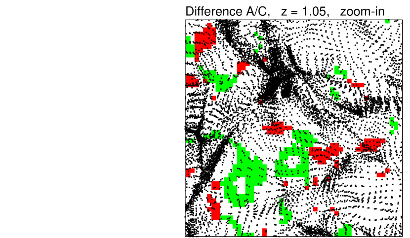
Figure 8.— Differential enrichment map between runs A and C, at redshift $z=1.05$. This figure shows a zoom-in of the upper right region of the third panel of figure 7.

3.2.1 Enrichment of Overdense vs. Underdense IGM

Figure 9.— Density statistics at redshift $z=3.38$ for runs A, B, and C. The quantities $N_{\rho}$, $N^{\rm rich}_{\rho}$, $N^{\rm rich}_{<\rho}$, and $N_{\rm ff}^{3}=256^{3}$ designate the number of cells (whether enriched or not) at a given density, the number of cells enriched by AGN outflows at a given density, the number of cells enriched by AGN outflows below a given density threshold, and the total number of cells in the computational volume, respectively. Top panel: histogram of the density distribution of cells. Second panel: number of cells enriched by AGN outflows at a given density, divided by the total number of cells in the computational volume. Third: number of cells enriched by AGN outflows at a given density, divided by the total number of cells at that density. Bottom: number of cells enriched by AGN outflows below a certain density threshold, divided by the corresponding number for the isotropic case ($\alpha=180^{\circ}$). The linestyles indicate the different opening angles: $\alpha=60^{\circ}$ (dashed), $120^{\circ}$ (dotted), $180^{\circ}$ (solid).

Figure 10.— Same as Figure 9, at redshift $z=2.57$.

Figure 11.— Same as Figure 9-10, at redshift $z=2.00$.

Figure 12.— Same as Figure 9-11, at redshift $z=1.05$.

Figure 13.— Same as Figure 9-12, at redshift $z=0.00$.

We investigate the relationship between metal enrichment by AGN outflows and the density of the regions being enriched, using runs A, B, and C. Figures 9 – 13 show various density statistics of the enriched regions at five different redshifts, $z=3.38,2.57,2.0,1.05$ and $0$, for 3 opening angles, $\alpha=60^{\circ},120^{\circ}$, and $180^{\circ}$. All quantities are plotted as functions of the overdensity (ratio of the local density to the mean density, $\rho/\rho_{\rm mean}$).

The top panels show the fractional number of cells in the whole grid (whether enriched or not) at a density $\rho$. The distribution resembles a skewed Gaussian, with more underdense volumes than overdense. The Gaussian becomes wider in time as large scale structures form in the cosmological volume, with further higher and lower densities being reached gradually. Most of the volume of the simulation box is underdense, and the peak of the distribution shifts to lower densities with time.

The second panels show the fractional number of cells which are enriched by AGN outflows ($N^{\rm rich}_{\rho}$). The enriched volume fraction is very small at early time, and increases with time, becoming significant from $z\sim 2-3$ and afterward. At a given redshift, we see a slight trend of the peak of the resulting Gaussian distribution shifted to lower densities for increasing anisotropy ($\alpha=180^{\circ},120^{\circ},60^{\circ}$). This indicates that more anisotropic outflows enrich underdense regions of the IGM. This is most noticeable at redshift $z=1.05$ (Fig. 12).

The third panels show the ratio of the cell counts in the second to the top panel, i.e., the number of cells enriched as the fraction of the total number of cells. In high-density regions ($\rho>\rho_{\rm mean}$) more isotropic outflow enrich larger volumes than anisotropic ones, while in low-density regions ($\rho<\rho_{\rm mean}$) we find exactly the opposite behavior. The effect is small, but most prominent at $z=1.05$. At $z=0$, dense regions are fully enriched for all values of $\alpha$, while at $z>2$ low-density regions are just starting to get enriched.

The bottom panels are cumulative versions of the second panels, showing the number of enriched cells below a given density threshold ($N^{\rm rich}_{<\rho}$), divided by the corresponding number $N^{\rm rich}_{<\rho,180}$ for isotropic outflows.. In low-density regions [$\log(\rho/\rho_{\rm mean})<0$], the ratio $N^{\rm rich}_{<\rho}/N^{\rm rich}_{<\rho,180}$ strongly depends on the opening angle, at all redshift but especially at early time ($z\geq 2$). The most anisotropic outflow ($\alpha=60^{\circ}$) enriches the largest underdense volumes, and the effect is stronger at lower densities. The effect is most prominent at earlier epochs ($z\sim 3.5-2$), and decreases in intensity with time, but is still visible at the present epoch. We explain this trend as follows. At earlier times, when the AGN outflows have just started to enrich the surrounding volumes, more anisotropic outflows enrich larger fractions of the lower density IGM, since these outflows expand along the direction of least resistance. As time goes on, large-scale structures form and grow, causing material to accrete from low- to high-density regions. This tends to even out the density of the enriched volumes, and as time goes on the effect of preferential enrichment of low-density regions by anisotropic outflows gets washed out. Such a trend in seen in our resulting density statistics, where the difference between the different opening angles is very small in Figure 13 at $z=0$.

3.2.2 Comparison with Pieri et al. 2007

The bottom 3 panels of Figures 9–13 are analogous to the plots in Figure 9 of PMG07. These authors considered outflows driven by SNe explosions in dwarf galaxies, and found that the anisotropy of the outflows had a major impact on the IGM enrichment in low-density regions. Outflows with opening angle $\alpha=60^{\circ}$ enriched the lowest-density regions of the IGM by a factor $3-4$ more than isotropic outflows. In this study, where we consider outflows driven by AGN in active galaxies, we find that a similar trend of increasingly anisotropic outflows to enrich lower-density regions, but the effect depends significantly on the redshift. The trend we obtained is not as dramatic as in PMG07 at the present epoch (Fig. 13), but becomes more and more prominent at earlier epochs. We find that at $z=2.57$ (Fig. 10), the factor by which outflows with $\alpha=60^{\circ}$ enrich low-density regions more than isotropic ones goes up to $1.7$. At $z=3.38$ (Fig. 9), the factor goes as high as $2.3$.

Even though we have used the same prescription for the anisotropic outflows as PMG07, we point out the following differences between the two studies. PMG07 did not perform an actual cosmological simulation. Instead, they generated an initial gaussian random field at high redshift, filtered that density field at various mass scales, and used the spherical collapse model to predict the collapse redshift of each halo (see Scannapieco & Broadhurst 2001 and PMG07 for details). This semi-analytical model has the advantage of simplicity, but does not include an accurate treatment of halo mergers and accretion of matter onto halo, and furthermore it underestimates the level of clustering of the halos (see, however, Pinsonneault et al. 2009). In this paper, we argue that the overlap between outflows, which results from the clustering of halos, is more important for isotropic outflows than anisotropic ones, and that accretion of low-density, metal-enriched matter onto dense structures tends to erase the effect of anisotropy. As a consequence, we find that the effect of anisotropy is still important at high redshifts, but greatly reduced at low redshifts.

3.3. AGN Lifetime

Figure 14.— Fractional volume ($N_{\rm rich}/N_{\rm ff}^{3}$) of simulation box enriched by AGN outflows as a function of redshift, for different AGN activity lifetimes: $T_{\rm AGN}=10^{7}{\rm yr}$ (dashed), $10^{8}{\rm yr}$ (solid), $10^{9}{\rm yr}$ (dotted). See §3.3 for details.

Table 2Runs with different active lifetimes $T_{\rm AGN}$

Run	$T_{\rm AGN}$ (yr)	Population Size	$N_{\rm rich}/N_{\rm ff}^{3}\;(z=0)$
D	$10^{7}$	$15\,279\,029$	1.00
C	$10^{8}$	$1\,535\,362$	0.83
E	$10^{9}$	$162\,228$	0.75

The simulations A, B, and C presented in the previous section all assumed that AGN activity lasts $T_{\rm AGN}=10^{8}{\rm yr}$. To study the effect of varying $T_{\rm AGN}$, we performed runs D and E, using AGN activity lifetimes of $T_{\rm AGN}=10^{7}{\rm yr}$ and $10^{9}{\rm yr}$, respectively. These values correspond to the lower limit and upper limit on $T_{\rm AGN}$ used by LG05. Simulations C, D, and E use the same opening angles, $\alpha=60^{\circ}$, and the same kinetic fraction, $\epsilon^{\phantom{1}}_{K}=0.1$, and differ only in the value of $T_{\rm AGN}$. We neglect any repeated activity (which might happen because of duty cycle) of the same AGN after it has become inactive, as did LG05. Considering duty cycles would have a small effect in our results, because of the way we model the outflow expansion and evolution (§2.5, our outflows continue to remain in the simulation box even after the central AGN has died).

A value of few $\times 10^{8}{\rm yr}$ is considered as the typical activity lifetime of the SMBH at the centers of active galaxies in other studies (e.g., Yu & Lu, 2008). A lifetime of $5\times 10^{8}{\rm yrs}$ has been used in theoretical modeling of radio galaxies by Blundell et al. (1999); Barai & Wiita (2007). Observations of X-ray activity in AGN (Barger et al., 2001), SDSS optical studies of active galaxies (Miller et al., 2003), and black hole demographics arguments (e.g., Marconi et al., 2004) all support an AGN activity lifetime of $\sim 10^{8}{\rm yr}$ or more (also, McLure & Dunlop, 2004).

Table 2 gives the parameters and results of runs C, D and E. The first and second columns give the run name and the value of $T_{\rm AGN}$ used, respectively. Column 3 gives the size of the AGN population, that is, the total number of sources obtained from the QLF (§2.2) in our cosmological volume over the Hubble time. The last column lists the resulting metal-enriched volume fractions at the present epoch. There are $\sim 10$ times more AGNs generated for a decrease of $T_{\rm AGN}$ by a factor of 10, since the QLF has to remain constant. This change in the number of sources makes a large difference in the resulting enriched volume fractions.

The redshift evolution of the enriched volume fractions for different active lifetimes are plotted in Figure 14. The largest AGN population ($T_{\rm AGN}=10^{7}{\rm yr}$) enriches significantly larger volume than the other two populations. In this case (run D) the fractional volume starts to become appreciable from $z\sim 3.5$, and grows afterward, such that $100\%$ of the volume of the box is enriched by $z\simeq 0.7$. The other two populations, with $T_{\rm AGN}=10^{8}$ and $10^{9}{\rm yr}$, enrich $0.83$ and $0.75$ of the volume at $z=0$, respectively. This result, that AGNs with shorter lifetimes enrich larger volumes than those with longer lifetimes, is opposite to what LG05 and Barai (2008) obtained. We explain this in the following, stressing the point that the method we employed to enrich our cosmological volumes is quite different from what other studies have used.

We use a dynamic particle enrichment scheme (§2.6), whereby we marked particles lying inside outflow volumes as enriched, assign a smoothing length to each of them, and calculate the volume of the box being filled by these enriched particles. In other studies (LG05 and Barai 2008) the enriched volume fraction is calculated by finding the fraction of the computational volume which is located inside the geometrical boundaries of the outflows. In our approach, particles that are metal-enriched by outflows are allowed to move, and might move to regions not intercepted by an outflow. This increases the chance of enriching a larger fraction of the total volume. The trend heightens when the number of outflows increase; as more AGN are born they are placed in distinct locations distributed throughout the box (according to §2.3), and they could potentially enrich larger volumes. This causes the enriched volume fraction to increase with increasing population size, even though the lifetime of each outflow is shorter.

3.4. Kinetic Fraction

Figure 15.— Fractional volume ($N_{\rm rich}/N_{\rm ff}^{3}$) of simulation box enriched by AGN outflows as a function of redshift, for different kinetic fractions: $\epsilon_{K}=0.1$ (solid), $0.05$ (dashed), $0.01$ (dotted). See §3.4 for details.

In runs F and G, we consider different values of the kinetic fraction (the fraction of the AGN bolometric luminosity which converts to the kinetic luminosity of the jets, §2.5), $\epsilon_{K}=0.05$ and $0.01$, in addition to our standard value $\epsilon^{\phantom{1}}_{K}=0.1$ (run C). Comparing with other studies, FL01 used a value $\epsilon^{\phantom{1}}_{K}=0.1$. LG05 first experimented with a value $\epsilon^{\phantom{1}}_{K}=0.1$, and found an enriched volume fraction that was too large to agree with observations, so later they chose $\epsilon^{\phantom{1}}_{K}=0.01$ as their fiducial value. Hence, we are sampling the range of values that have been considered in other studies.

The resulting enriched volume fractions are plotted in Figure 15 as a function of redshift, for the different kinetic fractions. We find the same general trend as in runs A – E, namely that the enriched volume fraction is small at $z>2$, and then grows rapidly afterward up to the present. At $z=0$, fractions of 0.83, 0.79, and 0.71 of the volume are enriched by outflows with $\epsilon^{\phantom{1}}_{K}=0.1$, 0.05, and 0.01, respectively.

Using their model for the AGN outflows, LG05 found that the cosmological volume is completely filled ($100\%$) by $z\sim 2$ when using $\epsilon_{K}=0.1$ or $0.05$, and with $\epsilon_{K}=0.01$, their volume filling fraction at $z=0$ is $80\%$. The enriched volume fractions we obtained with $\epsilon_{K}=0.1$ and $0.05$ are comparable to those obtained by LG05 with $\epsilon_{K}=0.01$. With $\epsilon_{K}=0.01$, we obtained an enriched volume fraction $\sim 10\%$ smaller than that of LG05. We find that decreasing the kinetic fraction by a factor of 10 reduces the volume enriched by $\approx 12\%$. This is comparable to a corresponding $\approx 20\%$ reduction in the volume filling fraction found by LG05 (their Fig. 3), when $\epsilon_{K}$ is reduced by a factor of 10. It may seem surprising that increasing by a factor of 10 the energy driving the expansion of the outflows has only a $\sim 14\%$ effect on the final results. With a larger kinetic fraction, outflows are certainly larger, but also overlap more with one another. The lowest-density regions, located far from any AGN, still manage to escape enrichment.

3.5. Bias in AGN Location

Figure 16.— Fractional volume ($N_{\rm rich}/N_{\rm ff}^{3}$) of simulation box enriched by AGN outflows as a function of redshift, The linestyles indicate different methods of AGN location: Default run C (solid), run H with bias parameter $\psi=2$, as in LG05 (dotted), run I, biased to densest peaks (dashed). See §3.5 for details.

AGNs are observed to be clustered in the universe, with the clustering amplitude increasing with redshift (Porciani et al., 2004; Croom et al., 2005; Shen et al., 2007). We study the effect of bias in the distribution of AGNs by considering two different methods for spatially locating the AGNs inside the computational volume, in addition to our original method (§2.3) used in runs A–G.

In run H, we use a location biasing condition similar to that used by LG05, but restricted to cells containing a local density peak (this is required by our method for finding the direction of last resistance as discussed in §2.3). We calculate the probability of each peak cell of hosting an AGN as

$${\cal P}=\frac{\rho^{\psi}}{\sum_{1}^{N_{\rm peak}}\left(\rho^{\psi}\right)}\,,$$ (16)

where $\rho$ is the filtered density (see §2.3) of the cell, $N_{\rm peak}$ is the number of available density peaks (not containing an AGN already) inside the computational volume, and $\psi$ is the bias parameter, which is denoted by $\alpha$ in equation (2) of LG05. The summation in the denominator of equation (16) is over all the density peaks at the relevant timestep. We use a constant bias value $\psi=2$, as did LG05 in their fiducial run. At each timestep, we use a Monte Carlo rejection method to locate the AGNs randomly, with a probability given by equation (16).

In run I, we bias the AGNs in favor of the highest-density peaks inside the cosmological volume. At each timestep, we find all the peak cells (§2.3), and then sort them in descending order of their density. The new AGNs (those born in that timestep) are located in the peak cells which have the highest densities. We start with the highest-density peak and locate one AGN (selected randomly from the ones just born) in it, go to the next highest-density peak cell and repeat the process, until all AGNs have been assigned locations. Notice that the methods used in simulations C and I effectively correspond to bias parameters $\psi=0$ and $\psi\rightarrow\infty$, respectively.

Figure 16 shows the redshift evolution of the enriched volume fraction for the different location methods. The enriched volume fraction decreases with increasing bias, at all redshifts. At $z=0$, the enriched volume fraction reaches 0.83 for the case without bias ($\psi=0$, run C), 0.75 for the intermediate case ($\psi=2$, run H), and $0.65$ for the maximum bias case ($\psi\rightarrow\infty$, run I). Such a behavior is expected, as with the introduction of gradual bias AGNs are increasingly clustered in high-density regions, so their outflows tend to overlap. Biasing to the highest density peaks reduces the present enriched volume fraction by 18% compared with the default case.

4. SUMMARY AND CONCLUSION

We have implemented a semi-analytical model of anisotropic AGN outflows in cosmological N-body simulations. The AGNs are placed at the location of local density peaks, and the outflows are allowed to expand anisotropically from those peaks, along the direction of least resistance, with a biconical geometry. Each AGN produces an outflow from its birth, which at first expands rapidly in the active-AGN phase for a time $T_{\rm AGN}$ until the AGN turns off, and then continues to expand slowly due to its overpressure. Finally after coming to pressure equilibrium with the external IGM the outflow simply follows the Hubble flow. The outflows carry with them metals produced by stars in the host galaxy, and enrich the regions of the IGM that they intercept. We used this algorithm to simulate the evolution of the large-scale structure and the propagation of outflows inside a cosmological volume of size ($128~{}h^{-1}$ Mpc)³, from initial redshift $z=24$ to final redshift $z=0$, in a concordance $\Lambda$CDM model. We performed a total of 9 simulations, varying the opening angle of the outflows, the active lifetime of the AGNs, the kinetic fraction, and the method used for locating the AGNs inside the cosmological volume.

(1) The enriched volume fractions (fraction by volume of the IGM enriched in metals by the outflows) are small at $z\gtrsim 2.5$, and then grow rapidly afterward up to $z=0$. In our simulations with different parameter values, we found that AGN outflows enrich $0.65-1.0$ of the total volume of the universe by the present epoch.

(2) The enriched volume fractions do not depend significantly on the opening angle of the outflows. More anisotropic outflows (smaller $\alpha$) are found to enrich slightly larger volumes than more isotropic ones, because the anisotropic ones grow bigger in radius and have less overlap. Increasingly anisotropic AGN outflows enrich lower-density volumes of the IGM, to an extent that depends on redshift. The trend is most prominent at earlier epochs, and not very dramatic but still visible at the present. Outflows with opening angles $\alpha=60^{\circ}$ enrich the underdense IGM more than isotropic outflows by a factor of $2.3$ at $z=3.38$, and $1.7$ at $z=2.57$. Initially, high-density regions get enriched by outflows, since the AGNs producing these outflows are located predominantly in these regions. Eventually, expanding outflows reach low-density regions of the IGM, and these regions also get enriched. This effect is larger for more anisotropic outflows, since these outflows expand along the directions of least resistance, reaching the low-density regions sooner and more easily. That enriched matter, located in underdense regions at earlier epochs, gravitationally accretes into higher-density regions with time, as large-scale structures grow. As a result, the effect of preferential enrichment of underdense IGM by more anisotropic outflows gets washed out with time, such that the difference is quite small at the present, even though it is quite significant at redshifts $z>1$.

(3) Reducing the active lifetime $T_{\rm AGN}$ of the AGNs results in larger enriched volume fractions. Any reduction in $T_{\rm AGN}$ must be accompanied by a corresponding increase in the number of AGNs, such that the observed QLF remains the same. When the number of sources increases, these sources tend to be distributed more uniformly throughout the computational volume, resulting in a more efficient enrichment. With $T_{\rm AGN}=10^{7}{\rm yr}$, 100% of the volume is enriched by redshift $z=0.7$.

(4) The enriched volume fractions for kinetic fractions $\epsilon^{\phantom{0}}_{K}=0.1,0.05$ and $0.01$ are $0.83,0.79$ and $0.71$, respectively, at the present epoch. This is consistent with the results reported by LG05. Increasing $\epsilon^{\phantom{0}}_{K}$ results in larger outflows, but the main consequence is to increase the level of overlap, rather than the enriched volume fraction.

(5) We varied the prescription for locating AGNs in the computational volume by introducing a bias parameter which favors high-density peaks. This increases the level of clustering of the AGNs, and when AGNs are more clustered, there is more overlap between outflows, resulting in a lower enriched volume fraction at all redshifts. The maximum effect is an 18% decrease at $z=0$ when going from an unbiased distribution to a maximally biased one.

This paper focused on the metal-enriched volume fraction by the outflows. In a forthcoming paper, we will focus on the metal abundances in the IGM resulting from anisotropic AGN outflows, and their observational consequences.

Appendix A NUMERICAL SOLUTION FOR THE OUTFLOW

In this appendix, we describe the technique used for solving the equations describing the evolution of the outflows. The presentation closely follows the one used in the appendix of PMG07.

The equations governing the evolution of the outflow are

$$\ddot{R} = {4\pi R^{2}[1-\cos(\alpha/2)]\over M_{s}}(p^{\phantom{1}}_{T}+p^{\phantom{1}}_{B}-p^{\phantom{1}}_{x})-{G\over R^{2}}\left[M_{\rm gal}+{M_{s}\over 2}\right]-{\Omega(z)H(z)^{2}R\over 2}$$ (A1)

$$+\Omega_{\Lambda}(z)H^{2}(z)R-{\dot{M}_{s}\over M_{s}}[\dot{R}-v_{p}(R)]\,,$$

$$\dot{M}_{s} = \cases{0\,,&$v_{p}(R)\geq\dot{R}$,\cr\displaystyle{3\Omega_{b}(z)H^{2}(z)R^{2}\over 2G}\left(1-\cos{\alpha\over 2}\right)[\dot{R}-v_{p}(r)]\,,&$v_{p}(R)<\dot{R}$,\cr}$$ (A2)

$$\dot{p}^{\phantom{1}}_{T} = {\Lambda\over 2\pi R^{3}[1-\cos(\alpha/2)]}-5p^{\phantom{1}}_{T}{\dot{R}\over R}\,,$$ (A3)

$$\dot{p}^{\phantom{1}}_{B} = {\epsilon^{\phantom{1}}_{B}L_{\rm AGN}\over 4\pi R^{3}[1-\cos(\alpha/2)]}-4p^{\phantom{1}}_{B}{\dot{R}\over R}\,.$$ (A4)

with the initial conditions $R=0$ at $t=0$. We used equations (8) and (11) to eliminate $M_{d}$ and $\rho_{x}$ in equations (A1) and (A2). Notice that since $M_{s}\propto 1-\cos(\alpha/2)$, the dependencies of the opening angle $\alpha$ cancel out in the first and last terms of equation (A1). The only remaining term in that equation that depends on $\alpha$ is the term $-GM_{s}/2R^{2}$. The most important dependencies on $\alpha$ are found in equations (A3) and (A4). The energies (thermal and magnetic) are injected into smaller volumes, leading to larger pressures.

Many terms in equations (A1)–(A4) diverge at $t=0$, making it impossible to find a numerical solution in this form (these divergences occur because we neglect the finite size of the source; in the real universe, many terms are large, but finite, at a radius $R$ that it small, but nonzero). To improve the behavior of the equations at early time, we perform a change of variable. To find the appropriate change of variable, we take the limit $t\rightarrow 0$ in equations (A1)–(A4), and keep only the leading terms. We get

$$\ddot{R} = {4\pi R^{2}[1-\cos(\alpha/2)](p^{\phantom{1}}_{T}+p^{\phantom{1}}_{B})\over M_{s}}-{\dot{M}_{s}\dot{R}\over M_{s}}\,,$$ (A5)

$$\dot{M}_{s} = 4\pi R^{2}[1-\cos(\alpha/2)]\rho_{x,i}\dot{R}\,,$$ (A6)

$$\dot{p}^{\phantom{1}}_{T} = {\Lambda_{i}\over 2\pi R^{3}[1-\cos(\alpha/2)]}-5p^{\phantom{1}}_{T}{\dot{R}\over R}\,,$$ (A7)

$$\dot{p}^{\phantom{1}}_{B} = {\epsilon^{\phantom{1}}_{B}\Lambda_{i}\over 4\pi R^{3}[1-\cos(\alpha/2)]}-4p^{\phantom{1}}_{B}{\dot{R}\over R}\,.$$ (A8)

where the subscripts $i$ indicates initial values at $t=0$. Notice that in equation (A8), we used $L_{\rm AGN}=\Lambda$ in the limit $t\rightarrow 0$. We can easily show that the solutions of equations (A5)–(A8) are power laws,

$$R = Ct^{3/5}\,,$$ (A9)

$$M_{s} = {4\pi C^{3}[1-\cos(\alpha/2)]\rho_{x,i}\over 3}t^{9/5}\,,$$ (A10)

$$p^{\phantom{1}}_{T} = {7C^{2}\rho_{x,i}\over 25(1+\epsilon^{\phantom{1}}_{B}/2)}t^{-4/5}\,,$$ (A11)

$$p^{\phantom{1}}_{B} = {7C^{2}\rho_{x,i}\over 25(1+2/\epsilon^{\phantom{1}}_{B})}t^{-4/5}\,,$$ (A12)

where

$$C=\left\{{125\Lambda_{i}(1+\epsilon^{\phantom{1}}_{B}/2)\over 154\pi\rho_{x,i}[1-\cos(\alpha/2)]}\right\}^{1/5}\,.$$ (A13)

Using equations (A9)–(A12), we can find the proper change of variables. We define

$$S = Rt^{2/5}\,,$$ (A14)

$$N_{s} = M_{s}t^{-4/5}\,,$$ (A15)

$$q^{\phantom{1}}_{T} = p^{\phantom{1}}_{T}t^{9/5}\,,$$ (A16)

$$q^{\phantom{1}}_{B} = p^{\phantom{1}}_{B}t^{9/5}\,,$$ (A17)

$$U = \dot{S}t\,,$$ (A18)

$$O_{s} = \dot{N}_{s}t\,.$$ (A19)

In the limit $t\rightarrow 0$, the six functions $S$, $N_{s}$, $q^{\phantom{1}}_{T}$, $q^{\phantom{1}}_{B}$, $U$, and $O_{s}$ vary linearly with $t$. We now eliminate the functions $R$, $M_{s}$, $p^{\phantom{1}}_{T}$ and $p^{\phantom{1}}_{B}$ in our original equations (A1)–(A4) using equations (A14)–(A19) and get

$$\dot{U} = {9U\over 5t}-{14S\over 25t}+{4\pi S^{2}(q^{\phantom{1}}_{T}+q^{\phantom{1}}_{B}-q^{\phantom{1}}_{x})\over N_{s}t^{2}}\left(1-\cos{\alpha\over 2}\right)-{GM_{\rm gal}t^{11/5}\over S^{2}}-{\Omega H^{2}St\over 2}$$ (A20)

$$-{GN_{s}t^{3}\over 2S^{2}}+\Omega_{\Lambda}H^{2}St-\left[{O_{s}\over N_{s}}+{4\over 5}\right]\left[{U\over t}-{2S\over 5t}-HS\right]\,,$$

$$\dot{N}_{s} = \cases{\displaystyle-{4N_{s}\over 5t}\,,&$\displaystyle HSt+{2S\over 5}\geq U$,\cr\displaystyle{3\Omega_{b}H^{2}S^{2}\over 2G}\left(1-\cos{\alpha\over 2}\right)\left[{U\over t^{3}}-{2S\over 5t^{3}}-{HS\over t^{2}}\right]-{4N_{s}\over 5t}\,,&$\displaystyle HSt+{2S\over 5}<U$,\cr}$$ (A21)

$$\dot{q}^{\phantom{1}}_{T} = {\Lambda t^{3}\over 2\pi S^{3}[1-\cos(\alpha/2)]}-{5q^{\phantom{1}}_{T}U\over St}+{19q^{\phantom{1}}_{T}\over 5t}\,,$$ (A22)

$$\dot{q}^{\phantom{1}}_{B} = {\epsilon^{\phantom{1}}_{B}L_{\rm AGN}\,t^{3}\over 4\pi S^{3}[1-\cos(\alpha/2)]}-{4q^{\phantom{1}}_{B}U\over St}+{17q^{\phantom{1}}_{B}\over 5t}\,,$$ (A23)

$$\dot{S} = {U\over t}\,,$$ (A24)

where $q^{\phantom{1}}_{x}\equiv p^{\phantom{1}}_{x}t^{9/5}$ in equation (A20).

These equations are completely equivalent to our original equations (A1)–(A4), but all divergences at $t=0$ have been eliminated. These equations can therefore be integrated numerically using a standard Runge-Kutta algorithm, with the initial conditions $U=S=N_{s}=q^{\phantom{1}}_{T}=q^{\phantom{1}}_{B}=0$ at $t=0$. However, before doing so, it is preferable to rewrite the equations in dimensionless form. We define

$$\tau \equiv H_{0}t\,,$$ (A25)

$$\tilde{S} \equiv {H_{0}S\over C}\,,$$ (A26)

$$\tilde{U} \equiv {H_{0}U\over C}\,,$$ (A27)

$$\tilde{N}_{s} \equiv {GN_{s}\over C^{3}H_{0}}\,,$$ (A28)

$$\tilde{O}_{s} \equiv {GO_{s}\over C^{3}H_{0}}\,,$$ (A29)

$$\tilde{q}^{\phantom{1}}_{T} \equiv {Gq^{\phantom{1}}_{T}\over C^{2}H_{0}}\,,$$ (A30)

$$\tilde{q}^{\phantom{1}}_{B} \equiv {Gq^{\phantom{1}}_{B}\over C^{2}H_{0}}\,,$$ (A31)

$$\tilde{q}^{\phantom{1}}_{x} \equiv {Gq^{\phantom{1}}_{x}\over C^{2}H_{0}}\,,$$ (A32)

$$f_{H} \equiv {H\over H_{0}}\,,$$ (A33)

$$f_{\Lambda} \equiv {\Lambda\over\Lambda_{i}}\,,$$ (A34)

$${\cal M} \equiv {GM_{\rm gal}\over C^{3}H_{0}^{1/5}}\,.$$ (A35)

Equations (A20)–(A24) reduce to their dimensionless form,

$${d\tilde{U}\over d\tau} = {9\tilde{U}\over 5\tau}-{14\tilde{S}\over 25\tau}+{4\pi\tilde{S}^{2}(\tilde{q}^{\phantom{1}}_{T}+\tilde{q}^{\phantom{1}}_{B}-\tilde{q}^{\phantom{1}}_{x})\over\tilde{N}_{s}\tau^{2}}\left(1-\cos{\alpha\over 2}\right)-{{\cal M}\tau^{11/5}\over\tilde{S}^{2}}-{\Omega f_{H}^{2}\tilde{S}\tau\over 2}$$ (A36)

$$-{\tilde{N}_{s}\tau^{3}\over 2\tilde{S}^{2}}+\Omega_{\Lambda}f_{H}^{2}\tilde{S}\tau-\left[{\tilde{O}_{s}\over\tilde{N}_{s}}+{4\over 5}\right]\left[{\tilde{U}\over\tau}-{2\tilde{S}\over 5\tau}-f_{H}\tilde{S}\right]\,,$$

$${d\tilde{N}_{s}\over d\tau} = \cases{\displaystyle-{4\tilde{N}_{s}\over 5\tau}\,,&$\displaystyle f_{H}\tilde{S}\tau+{2\tilde{S}\over 5}\geq\tilde{U}$,\cr\displaystyle{3f_{H}^{2}\Omega_{b}\tilde{S}^{2}\over 2}\left(1-\cos{\alpha\over 2}\right)\left[{\tilde{U}\over\tau^{3}}-{2\tilde{S}\over 5\tau^{3}}-{f_{H}\tilde{S}\over\tau^{2}}\right]-{4\tilde{N}_{s}\over 5\tau}\,,&$\displaystyle f_{H}\tilde{S}\tau+{2\tilde{S}\over 5}<\tilde{U}$,\cr}$$ (A37)

$${d\tilde{q}^{\phantom{1}}_{T}\over d\tau} = {231f_{Hi}^{2}\Omega_{bi}f^{\phantom{1}}_{\Lambda}\tau^{3}\over 1000\pi\tilde{S}^{3}(1+\epsilon^{\phantom{1}}_{B}/2)}-{5\tilde{q}^{\phantom{1}}_{T}\tilde{U}\over\tilde{S}\tau}+{19\tilde{q}^{\phantom{1}}_{T}\over 5\tau}\,,$$ (A38)

$${d\tilde{q}^{\phantom{1}}_{B}\over d\tau} = {231f_{Hi}^{2}\Omega_{bi}f^{\phantom{1}}_{\Lambda}\tau^{3}\over 1000\pi\tilde{S}^{3}(1+2/\epsilon^{\phantom{1}}_{B})}-{4\tilde{q}^{\phantom{1}}_{B}\tilde{U}\over\tilde{S}\tau}+{17\tilde{q}^{\phantom{1}}_{B}\over 5\tau}\,,$$ (A39)

$${d\tilde{S}\over d\tau} = {\tilde{U}\over\tau}\,,$$ (A40)

where $\tilde{O}_{s}\equiv\tau(d\tilde{N}_{s}/d\tau)$ in equation (A36). In the limit $\tau\rightarrow 0$, where many terms take the form $0/0$, the derivatives reduce to $d\tilde{S}/d\tau=d\tilde{U}/d\tau=1$, $d\tilde{q}^{\phantom{1}}_{T}/d\tau=21\Omega_{b,i}f^{2}_{H,i}/200\pi(1+\epsilon_{B}/2)$, $d\tilde{q}^{\phantom{1}}_{B}/d\tau=21\Omega_{b,i}f^{2}_{H,i}/200\pi(1+2/\epsilon_{B})$, and $d\tilde{N}_{s}/d\tau=\Omega_{b,i}f^{2}_{H,i}\left(1-\cos\alpha/2\right)/2$.

The quantity $f_{\Lambda}$ appearing in equations (A38) and (A39) depends on the luminosity $L_{\rm Comp}$, which is given by equation (14). We eliminate $P_{T}$ and $R$ in equation (14), using equations (A14), (A16), (A25), (A26), and (A30), then eliminate $C$ using equation (A13). We get

$${L_{\rm Comp}\over L_{i}}={200\pi^{3}\over 2079}{\sigma_{T}\hbar\over m_{e}H_{0}\Omega_{b,i}f^{2}_{H,i}}{\left(kT_{\gamma 0}\over\hbar c\right)^{4}}{\left(1+z\right)^{4}}{\tilde{q}_{T}\tilde{S}^{3}\over\tau^{3}}\,.$$ (A41)

References

- Anathpindika & Whitworth (2008) Anathpindika, S., & Whitworth, A. P. 2008, A&A, 487, 605
- Antonuccio-Delogu & Silk (2008) Antonuccio-Delogu, V., & Silk, J. 2008, MNRAS, 389, 1750
- Barai (2008) Barai, P. 2008, ApJ, 682, L17
- Barai & Wiita (2007) Barai, P., & Wiita, P. J. 2007, ApJ, 658, 217
- Barger et al. (2001) Barger, A. J. et al. 2001, AJ, 122, 2177
- Begelman & Cioffi (1989) Begelman, M. C., & Cioffi, D. F. 1989, ApJ, 345, L21
- Begelman (2004) Begelman, M. C. 2004, in Coevolution of black Holes and Galaxies, Carnegie Observatories Astrophysics Series, ed. L. C. Ho, p. 374
- Begelman & Nath (2005) Begelman, M. C., & Nath, B. B. 2005, MNRAS, 361, 1387
- Best (2007) Best, P. N. 2007, NewAR, 51, 168
- Bicknell et al. (2000) Bicknell, G. V. et al. 2000, ApJ, 540, 678
- Blundell et al. (1999) Blundell, K. M., Rawlings, S., & Willott, C. J. 1999, AJ, 117, 677
- Blustin et al. (2005) Blustin, A. J., Page, M. J., Fuerst, S. V., Branduardi-Raymont, G. & Ashton, C. E. 2005, A&A, 431, 111
- Bower et al. (2006) Bower, R. G. et al. 2006, MNRAS, 370, 645
- Chartas et al. (2003) Chartas, G., Brandt, W. N., & Gallagher, S. C. 2003, ApJ, 595, 85
- Chartas et al. (2007) Chartas, G., Brandt, W. N., Gallagher, S. C., & Proga, D. 2007, AJ, 133, 1849
- Ciotti & Ostriker (2007) Ciotti, L., & Ostriker, J. P. 2007, ApJ, 665, 1038
- Ciotti et al. (2009) Ciotti, L., Ostriker, J. P. & Proga, D. 2009, ApJ, submitted (arXiv: 0901.1089)
- Crenshaw et al. (1999) Crenshaw, D. M., Kraemer, S. B., Boggess, A., Maran, S. P., Mushotzky, R. F., & Wu, C.-C. 1999, ApJ, 516, 750
- Crenshaw et al. (2003) Crenshaw, D. M., Kraemer, S. B., & George, I. M. 2003, ARA&A, 41, 117
- Croom et al. (2005) Croom, S. M. et al. 2005, MNRAS, 356, 415
- Croston et al. (2008) Croston, J. H., Hardcastle, M. J., Kharb, P., Kraft, R. P., & Hota, A. 2008, ApJ, 688, 190
- Croton et al. (2006) Croton, D. J. et al. 2006, MNRAS, 365, 11
- Das et al. (2005) Das, V. et al. 2005, AJ, 130, 945
- Dasgupta et al. (2005) Dasgupta, S., Rao, A. R., Dewangan, G. C., & Agrawal, V. K. 2005, ApJ, 618, L87
- De Young (1989) De Young, D. S. 1989, ApJ, 342, L59
- Di Matteo et al. (2005) Di Matteo, T., Springel, V., & Hernquist, L. 2005, Nature, 433, 604
- D’Odorico et al. (2008) D’Odorico, V., Bruscoli, M., Saitta, F., Fontanot, F., Viel, M., Cristiani, S. & Monaco, P. 2008, MNRAS, 389, 1727
- Everett (2007) Everett, J. E. 2007, Ap&SS, 311, 269
- Ferrarese & Ford (2005) Ferrarese, L., & Ford, H. 2005, SSRv, 116, 523
- Fragile et al. (2004) Fragile, P. C., Murray, S. D., Anninos, P., & van Breugel, W. 2004, ApJ, 604, 74
- Furlanetto & Loeb (2001) Furlanetto, S. R., & Loeb, A. 2001, ApJ, 556, 619 (FL01)
- Ganguly & Brotherton (2008) Ganguly, R., & Brotherton, M. S. 2008, ApJ, 672, 102
- Gebhardt et al. (2000) Gebhardt, K. et al. 2000, ApJ, 539, L13
- Granato et al. (2004) Granato, G. L., De Zotti, G., Silva, L., Bressan, A., & Danese, L. 2004, ApJ, 600, 580
- Grenon (2007) Grenon, C., Master’s Thesis (Université Laval, 2007)
- Hickox et al. (2009) Hickox, R. C. et al. 2009, ApJ, in press (arXiv:0901.4121)
- Hinshaw et al. (2008) Hinshaw, G. et al. 2008, ApJS, 180, 225
- Hockney & Eastwood (1988) Hockney, R. W., & Eastwood, J. W. 1988, Computer Simulation Using Particles (New York: Adam Hilger).
- Hopkins et al. (2007) Hopkins, P. F., Richards, G. T., & Hernquist, L. 2007, ApJ, 654, 731
- Johansson et al. (2008) Johansson, P. H., Naab, T. & Burkert, A. 2008, conference proceedings, arXiv:0809.3399
- Juneau et al. (2005) Juneau, S. et al. 2005, ApJ, 619, L135
- Kauffmann et al. (2003) Kauffmann, G. et al. 2003, MNRAS, 346, 1055
- King (2003) King, A. 2003, ApJ, 596, L27
- Kormendy & Richstone (1995) Kormendy, J., & Richstone, D. 1995, ARA&A, 33, 581
- Kronberg et al. (2001) Kronberg, P. P., Dufton, Q. W., Li, H., & Colgate, S. A. 2001, ApJ, 560, 178
- Krongold et al. (2007) Krongold, Y., Nicastro, F., Elvis, M., Brickhouse, N., Binette, L., Mathur, S., & Jimenez-Bailon, E. 2007, ApJ, 659, 1022
- Laor (2000) Laor, A. 2000, ApJ, 543, L111
- Levine & Gnedin (2005) Levine, R., & Gnedin, N. Y. 2005, ApJ, 632, 727 (LG05)
- Mac Low & Ferrara (1999) Mac Low, M.-M., & Ferrara, A. 1999, ApJ, 513, 142
- Magorrian et al. (1998) Magorrian, J. et al. 1998, AJ, 115, 2285
- Marconi & Hunt (2003) Marconi, A., & Hunt, L. K. 2003, ApJ, 589, L21
- Marconi et al. (2004) Marconi, A., Risaliti, G., Gilli, R., Hunt, L. K., Maiolino, R., & Salvati, M. 2004, MNRAS, 351, 169
- Martel (2005) Martel, H. 2005, Technical Report UL-CRC/CTN-RT003 (astro-ph/0506540)
- Martel & Shapiro (2001a) Martel, H., & Shapiro, P. R. 2001a, RevMexAA, 10, 101
- Martel & Shapiro (2001b) Martel, H., & Shapiro, P. R. 2001b, in Relativistic Astrophysics, AIP Conference Proceedings 586, eds. J. C. Wheeler & H. Martel, p. 265
- McLure & Dunlop (2002) McLure, R. J., & Dunlop, J. S. 2002, MNRAS, 331, 795
- McLure & Dunlop (2004) McLure, R. J., & Dunlop, J. S. 2004, MNRAS, 352, 1390
- McNamara (2002) McNamara, B. R. 2002, NewAR, 46, 141
- McNamara & Nulsen (2007) McNamara, B. R., & Nulsen, P. E. J. 2007, ARA&A, 45, 117
- Mellema et al. (2002) Mellema, G., Kurk, J. D., & Rottgering, H. J. A. 2002, A&A, 395, L13
- Miller et al. (2003) Miller, C. J., Nichol, R. C., Gómez, P. L., Hopkins, A. M., & Bernardi, M. 2003, ApJ, 597, 142
- Murray et al. (2005) Murray, N., Quataert, E., & Thompson, T. A. 2005, ApJ, 618, 569
- Nath & Roychowdhury (2002) Nath, B. B., & Roychowdhury, S. 2002, MNRAS, 333, 145
- Nesvadba et al. (2008) Nesvadba, N. P. H., Lehnert, M. D., De Breuck, C., Gilbert, A. M., & van Breugel, W. 2008, A&A, 491, 407
- Nesvadba & Lehnert (2008) Nesvadba, N. P. H. & Lehnert, M. D. 2008, SF2A-2008, Proceedings of the annual meeting of the French Society of Astronomy and Astrophysics, eds. C. Charbonnel, F. Combes & R. Samadi, p 377
- O’Brien et al. (2005) O’Brien, P. T., Reeves, J. N., Simpson, C., & Ward, M. J. 2005, MNRAS, 360, L25
- Peterson (1997) Peterson, B. M. 1997, An introduction to active galactic nuclei, Cambridge (New York), Cambridge University Press
- Pieri et al. (2007) Pieri, M. M., Martel, H., & Grenon, C. 2007, ApJ, 658, 36 (PMG07)
- Pinsonneault et al. (2009) Pinsonneault, S., Pieri, M. M., & Martel, H. 2009, in preparation
- Pipino et al. (2009) Pipino, A., Silk, J., & Matteucci, F. 2009, MNRAS, 392, 475
- Polletta et al. (2008) Polletta, M. et al. 2008, A&A, 492, 81
- Porciani et al. (2004) Porciani, C., Magliocchetti, M., & Norberg, P. 2004, MNRAS, 355, 1010
- Pounds et al. (2003) Pounds, K. A., King, A. R., Page, K. L., & O’Brien, P. T. 2003, MNRAS, 346, 1025
- Rafter et al. (2009) Rafter, S. E., Crenshaw, D. M., & Wiita, P. J. 2009, AJ, 137, 42
- Recchi et al. (2009) Recchi, S., Hensler, G. & Anelli, D. 2009, in Star-forming Dwarf Galaxies: Ariane’s Thread in the Cosmic Labyrinth, in press (arXiv: 0901.1976)
- Rees (1989) Rees, M. J. 1989, MNRAS, 239, 1P
- Reichard et al. (2003) Reichard, T. A. et al. 2003, AJ, 126, 2594
- Reynolds et al. (2002) Reynolds, C. S., Heinz, S., & Begelman, M. C. 2002, MNRAS, 332, 271
- Richards et al. (2002) Richards, G. T. et al. 2002, AJ, 124, 1
- Scannapieco & Broadhurst (2001) Scannapieco, E., & Broadhurst, T. 2001, ApJ, 549, 28
- Scannapieco & Oh (2004) Scannapieco, E., & Oh, S. P. 2004, ApJ, 608, 62 (SO04)
- Schawinski et al. (2007) Schawinski, K. et al. 2007, MNRAS, 382, 1415
- Schlesinger et al. (2009) Schlesinger, K., Pogge, R. W., Martini, P., Shields, J. C. & Fields, D. 2009, preprint (arXiv: 0902.0004)
- Shankar et al. (2008) Shankar, F., Cavaliere, A., Cirasuolo, M., & Maraschi, L. 2008, ApJ, 676, 131
- Shen et al. (2007) Shen, Y. et al. 2007, AJ, 133, 2222
- Silk & Rees (1998) Silk, J., & Rees, M. J. 1998, A&A, 331, L1
- Springel et al. (2005) Springel, V., Di Matteo, T., & Hernquist, L. 2005, ApJ, 620, L79
- Tegmark et al. (1993) Tegmark, M., Silk, J., & Evrard, A. 1993, ApJ, 417, 54
- van Breugel et al. (2004) van Breugel, W., Fragile, C., Anninos, P., & Murray, S. 2004, IAUS, 217, 472
- Willott et al. (1999) Willott, C. J., Rawlings, S., Blundell, K. M., & Lacy, M. 1999, MNRAS, 309, 1017
- Wyithe & Loeb (2003) Wyithe, J. S. B., & Loeb, A. 2003, ApJ, 595, 614
- Yu & Lu (2008) Yu, Q., & Lu, Y. 2008, ApJ, 689, 732