Detection of Earth-impacting asteroids
with the next generation all-sky surveys

Abstract

We have performed a simulation of a next generation sky survey’s (Pan-STARRS 1) efficiency for detecting Earth-impacting asteroids. The steady-state sky-plane distribution of the impactors long before impact is concentrated towards small solar elongations (Chesley & Spahr, 2004) but we find that there is interesting and potentially exploitable behavior in the sky-plane distribution in the months leading up to impact. The next generation surveys will find most of the dangerous impactors ($>$140 m diameter) during their decade-long survey missions though there is the potential to miss difficult objects with long synodic periods appearing in the direction of the Sun, as well as objects with long orbital periods that spend much of their time far from the Sun and Earth. A space-based platform that can observe close to the Sun may be needed to identify many of the potential impactors that spend much of their time interior to the Earth’s orbit. The next generation surveys have a good chance of imaging a bolide like 2008 TC₃ before it enters the atmosphere but the difficulty will lie in obtaining enough images in advance of impact to allow an accurate pre-impact orbit to be computed.

1 Introduction

Throughout most of human history it was not understood that the Earth has been battered by large asteroids and comets and that the impacts and subsequent environmental changes have serious consequences for the survival and evolution of life on the planet. But in the past $\sim$50 years more than 170 impact structures have been identified on the surface of the Earth (Earth-impact database, 2008). Were it not for the Earth’s protective atmosphere, oceans, erosion and plate tectonics, the surface of the Earth would be saturated with impact craters like most other atmosphereless solid bodies in our solar system. While the impact probability is now relatively well understood as a function of the impactor size (e.g.  Brown et al., 2002; Harris, 2007) this work addresses specific questions related to discovering impacting asteroids before they hit the Earth. In particular, we build upon the work of Chesley & Spahr (2004) and determine the sky-plane distribution of impacting asteroids before impact and the effectiveness of the next generation large synoptic sky surveys at identifying impactors.

The first surveys to target near-Earth objects (NEO) (Helin & Shoemaker, 1979), asteroids and comets with perihelion $<1.3$ AU, provided the first look at their orbit and size distribution and allowed the first determination of the impact rate from NEO statistics (Shoemaker, 1983) rather than crater counting on the Moon. These pioneers heightened the awareness of the impact risk and gave rise to the current generation of CCD-based asteroid and comet surveys such as Spacewatch (Gehrels, 1986), LINEAR (Stokes et al., 2000), LONEOS (Koehn & Bowell, 1999), NEAT (Pravdo et al., 1999), and the current leader in discovering NEOs, the Catalina Sky Survey (CSS) (Larson et al., 1998). These programs benefitted from the elevated impact risk perception when in 1998 the U.S. Congress followed the recommendations of Morrison (1992) and mandated that the U.S. National Aeronautics and Space Administration (NASA) search, find and catalog $\geq 90\%$ of NEOs with diameters larger than 1 km within 10 years. That goal will probably be achieved within the next few years. The residual impact risk is mainly due to the remaining undiscovered large asteroids and comets (Harris, 2007) but Stokes et al. (2004) suggest that the search should be expanded to identify $\geq 90$% of potentially hazardous objects (PHO) by 2020.

Stokes et al. (2004) showed that the extended goal cannot be achieved in a reasonable time frame with existing survey technology. The search needs to be done from space (rapid completion but at high risk and high cost) or from new ground-based facilities (slower completion but lower risk and lower cost). Their recommendation dovetailed nicely with the Astronomy and Astrophysics Survey Committee (2001) Decadal Report that made a strong case for the development of a large synoptic survey telescope (LSST) that would provide the necessary depth and sky coverage to identify the smaller PHOs while also satisfying the goals of other fields of astronomy.

There are currently a few candidates for a large synoptic survey telescope. The most ambitious is an 8.4 m system being designed by the eponymous LSSTC (the LSST Corporation) that anticipates beginning survey operations in 2016 in Chile. With a $\sim$9 deg² field of view and 15 s exposures, simulations suggest that their system could identify $\gtrsim$90% of PHOs in 15 years (Ivezić et al., 2007). A more modest LSST known as the Panoramic Survey Telescope and Rapid Response System (Pan-STARRS) will be composed of four 1.8m telescopes (PS4) and is expected to be located atop Mauna Kea in Hawaii. A prototype single telescope for Pan-STARRS known as PS1 should begin operations in mid-2009 from Haleakala, Maui. With a $\sim$7 deg² field of view, the excellent seeing from the summit of Mauna Kea, and the use of orthogonal transfer array CCDs (Burke et al., 2007) for on-chip image motion compensation, the Pan-STARRS system will be competitive with and completed earlier than the LSSTC’s system.

The next generation survey telescopes have the potential to be prolific discoverers of PHOs but Earthlings aren’t so much concerned with statistical impact risk calculated from PHO orbital distributions as they are interested in whether an impact event will occur. The statistical risk of a house burning down may seem inconsequential until you consider the actuality of your house being incinerated. Similarly, while Harris (2008) has calculated that expected fatalities due to an unanticipated asteroid impact have dropped from $\sim$1,100/year before the onset of modern NEO surveys to only $\sim$80/year now, as a species we would like to know whether one of the fatality inducing impacts will take place this century. Thus, this work concentrates on the detection of objects that may impact the Earth in the next hundred years.

Following Chesley & Spahr (2004) we concentrate on the subset of PHOs that are in fact destined for a collision with the Earth. They showed that long before impact the impactors’ steady state sky-plane distribution is concentrated on the ecliptic and at small solar elongation. We extend their analysis and find that the sky-plane distribution of impactors has interesting and potentially useful structure in the time leading to collision. We also study the capabilities of one next-generation survey (PS1) at identifying the impactors well before collision. In particular, we will answer the following questions: How different are the orbital characteristics of the impactor population and current NEO and PHO models? What is the survey efficiency for identifying asteroids on a collision course with the Earth as a function of their diameter? How much warning time will be provided before the impact? How accurate is the orbital solution prior to impact? How does the MOID evolve in time and is the current definition of a PHO consistent with flagging dangerous objects? What are the orbital properties of objects that are not found? Are there methods to improve the efficiency of identifying impactors? Given the size-frequency distribution of NEOs what is the probability that PS1 will actually identify an impactor and what will be its most probable size?

2 Synthetic Earth-impacting asteroids

Our synthetic impactor population model is described in detail in Chesley & Spahr (2004) and Grav et al. (2009). Here we provide a brief summary of the technique.

We created $\sim$130,000 impactors based on the NEO population developed by Bottke et al. (2000) and Bottke et al. (2002) hereafter referred to as the Bottke NEO Model. The model incorporates objects from both asteroidal and cometary source regions but has at least two problems that affect its utility for creating an impactor population: 1) it assumes that the orbit distribution of NEOs is independent of their diameter and 2) it provides the $(a,e,i,H)$ (semi-major axis, eccentricity, inclination, and absolute magnitude) distribution for NEOs on a coarse grid that is not suited to the narrower range of orbital elements of the impacting asteroids. However, there are few options to use as starting points for developing an impactor population and we will compare our impactor population’s orbit distribution to the known small impactor population to understand the limitations of our technique.

To generate the impactors NEOs were randomly selected from the Bottke NEO model and assigned random longitudes of ascending node and arguments of perihelion. Orbits with a MOID small enough to permit an impact were saved as potential impactors and then filtered according to their likelihood of impact to obtain the final set of impactors. The likelihood is the fraction of time that an object spends in close proximity to the Earth’s orbit. i.e. orbits with a small velocity relative to the Earth tend to have shorter impact intervals and higher intrinsic impact probabilities. Higher likelihoods received higher weighting in the selection. If an orbit was chosen as an impactor then a year of impact was randomly selected between 2010 and 2110 — the date of collision is already randomly fixed by the longitude of the node at impact. To this point, the process assumed a two-body asteroid orbit with no planetary perturbations. The final step was to ensure an impact under the influence of all the perturbations in a complete solar system dynamical model. This was done by differentially adjusting the two-body argument of perihelion ($\omega$) and orbital anomaly to reach a randomly selected target plane coordinate on the figure of the Earth. The final result is an osculating element set that leads to an Earth impact when propagated with the full dynamical model. The full set of impactors generate about three impacts per day uniformly distributed over the globe with an average separation of about 70 km.

This technique preferentially selects objects on Earth-like orbits out of the Bottke NEO model but Brasser & Wiegert (2008) show that objects do not remain long in these types of orbits. This is not a problem except in the sense addressed above — that the Bottke NEO model is provided on a relatively coarse grid — because the NEO model already accounts for NEO ‘residence times’ on all types of NEO orbits. However, since we assume a flat distribution of NEO orbit elements within the $(a,e,i)$ bin corresponding to Earth-like orbits it is likely that we generate fractionally more of the extremely Earth-like orbits than exist in reality.

As shown by Chesley & Spahr (2004) and in Fig. 1 there are important differences between the impactor population and the NEOs. The impactors have orbits with lower semi-major axis, inclination and eccentricity. This has the effect of decreasing the Earth encounter and impact velocity ($v_{\infty}$ and $v_{imp}$ respectively) for the impactors relative to the NEOs. The decreased impact velocity has implications for modelling the impact crater size-frequency distribution on the Earth and Moon since lower impact energies per unit mass require larger impactors to create equivalent-size craters.

As mentioned above, the Bottke NEO model assumed that the orbit distribution of the NEOs is independent of size. While this assumption is probably fine for large objects it must break down at smaller sizes due to the effect of non-gravitational forces such as the Yarkovsky effect (e.g.  Bottke et al., 1998; O’Brien & Greenberg, 2005). Where the transition occurs is not clear but Fig. 1 compares the $(a,e,i)$ distribution of our impactor population to sporadic fireballs from the IAU Meteor Database of photographic orbits (Lindblad et al., 2003). We removed fireballs due to 17 major meteor showers (Jenniskens, 2006) by requiring that the meteors not be associated with the parent meteor body using the dimensionless orbit similarity $D$-criterion of Valsecchi et al. (1999):

$$D^{2}=[U_{2}-U_{1}]^{2}+w_{1}[\cos\theta_{2}-\cos\theta_{1}]^{2}+\Delta\xi^{2},$$ (1)

where

$$\cos\theta = \frac{1-U^{2}-1/a}{2U},$$

$$\Delta\xi^{2} = \min\bigl{[}\;w_{2}\Delta\phi^{2}_{A}+w_{3}\Delta\lambda^{2}_{\oplus A},\;w_{2}\Delta\phi^{2}_{B}+w_{3}\Delta\lambda^{2}_{\oplus B}\;\bigr{]},$$

$$\phi_{A} = 2\sin\Bigl{(}\frac{\phi_{2}-\phi_{1}}{2}\Bigr{)},$$

$$\phi_{B} = 2\sin\Bigl{(}\frac{\pi+\phi_{2}-\phi_{1}}{2}\Bigr{)},$$

$$\lambda_{\oplus A} = 2\sin\Bigl{(}\frac{\lambda_{\oplus 2}-\lambda_{\oplus 1}}{2}\Bigr{)},$$

$$\lambda_{\oplus B} = 2\sin\Bigl{(}\frac{\pi+\lambda_{\oplus 2}-\lambda_{\oplus 1}}{2}\Bigr{)}.$$

The 1 and 2 subscripts refer to the two bodies whose orbits are being compared, U is the unperturbed geocentric speed just prior to impact, ($\theta$, $\phi$) define the direction of the radiant in a frame moving with the Earth about the Sun, and $\lambda_{\oplus}$ is the ecliptic longitude of the Earth at the time of meteoroid impact. The weighting factors $w_{i}$ were set to 1 as per Valsecchi et al. (1999). All objects with $D$-criterion relative to a parent body of $\leq 0.2$ were discarded (577 meteors) leaving 2002 sporadic background fireballs.

The impactor and NEO orbit distributions have already been discussed briefly above and in detail by Chesley & Spahr (2004). The differences between the impactor population and the fireballs are perhaps more interesting where it is important to keep in mind that the comparison in Fig. 1 is between the bias corrected impactor population and the observed bolide population. We believe that the apparent difference between the impactor and bolide distributions is a consequence of the uncorrected observational selection effects in the bolide data along with modifications in the distributions due to the Yarkovsky effect (e.g.  Farinella et al., 1998). The bolide detection technique has a strong bias towards high kinetic energy events that preferentially detects objects on cometary-like orbits (Ceplecha et al., 1998). Indeed, if we consider ‘comets’ to be objects from our sporadic bolide data with $a>4$ AU or $e>0.9$ or $i>90\hbox{${}^{\circ}$}$ then $\sim$13.4% of the objects are of ‘cometary’ origin. This value is about twice the cometary fraction of $6\pm 4$% suggested by the Bottke NEO model and consistent with the expected ‘comet’ enhancement in the bolide data. On the other hand, it is only half the 25% cometary contribution suggested by Stuart & Binzel (2004).

No meteor or fireball had ever been detected before entering the Earth’s atmosphere before we generated our synthetic population of Earth-impacting asteroids. Then, on 7 October 2008, asteroid 2008 TC₃ was discovered by CSS using their 1.5 m telescope. Rapid followup by other observatories made it almost immediately clear that the few-meter-diameter ($H=30.7$) asteroid would enter the Earth’s atmosphere within a day and explode over northern Sudan. The substantial and largely self-organized follow-up effort resulted in 789 astrometric observations from amateur and professional observatories worldwide being submitted to the Minor Planet Center. Due to the parallax induced by the distance between the observatories and the proximity of the asteroid, the observations allowed an accurate pre-impact orbit to be computed despite the short observational timespan (Table 1). The pre-impact orbit is very consistent with our predicted impactor orbit distribution as shown in Fig. 1. Note that, in particular for the eccentricity, the pre-impact orbit matches the expected impactor population better than the debiased NEO population or the observed bolide population.

Orbital elements and their uncertainties for 20080TC3
	$a$ [AU]	$e$	$i$ [∘]	$\Omega$ [∘]	$\omega$ [∘]	$M_{0}$ [∘]
Elements	1.2712175	0.2856863	2.331633	194.1308964	233.954719	328.58963
1-$\sigma$ unc	0.0000031	0.0000023	0.000017	0.0000011	0.000040	0.00015

Table 1: Keplerian elements and their 1-$\sigma$ uncertainties for 2008 TC₃ for the epoch 2008 Oct 6.11535 TT, about one day before atmospheric entry on 2008 Oct 7.1146 UTC. The orbital solution made use of 574 astrometric observations (42 of which were discarded as outliers) and assumed an uncorrelated astrometric uncertainty of 0.5 arcseconds for every measurement. The orbital solution was obtained using the OpenOrb software (Granvik et al., 2008).

2.1 Time evolution of the impactor population’s MOIDs

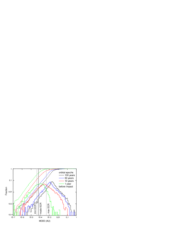
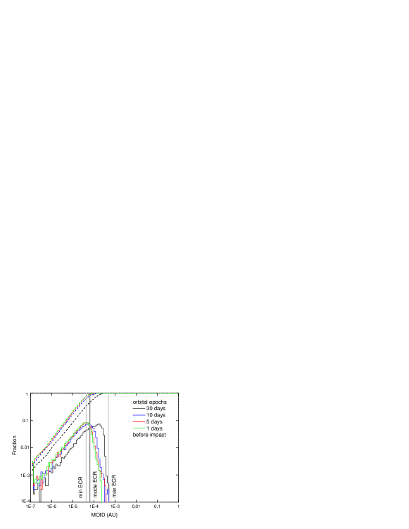
Figure 2: Fractional differential (solid) and cumulative (dashed) distribution of MOID for synthetic impactors at different times before impact. The Earth capture radius (ECR) is calculated for the highest (max ECR), most probable (mode ECR) and lowest (min ECR) impactor encounter velocity. The bin size is $\log(MOID/AU)=0.07$ in both figures.

Recall that a PHO is defined as an object with $H\leq 22$ and a MOID $<0.05$ AU with respect to the Earth’s orbit. We investigated the evolution of the MOID for our impactor population as a function of time before impact as shown in Fig. 2. All the impactors’s osculating orbits were integrated using the JPL’s N-body integrator incorporating the effects of the Sun, eight planets, and the dwarf planets Pluto, Ceres, Vesta and Pallas. MOIDs were then calculated at different times before impact using the synthetic objects’s integrated osculating orbits at the time of interest, not the orbit derived from synthetic observations of the object. We see that as the time of impact approaches the MOID decreases such that one month before impact essentially all objects have a MOID less than the Earth’s capture radius ($b$):

$${b={R\cdot\sqrt{{1+\frac{v_{e}^{2}}{v_{\infty}^{2}}}}}},$$ (2)

where $v_{e}$ represents the escape velocity from the surface of the Earth. Fig. 3 shows that $\sim$99% of all impactors are identified as PHOs 45 years in advance of impact. Even 100 years before impact $\sim$98% of the objects have a MOID$<$0.05 AU though the fraction of non-PHO impactors is increasing rapidly as the time before impact increases.

There are a few objects with MOID$>$0.05 AU that would not be identified as impactors or PHOs using a single MOID determination from a derived osculating orbit at the time of discovery. These objects suffer from a close approach to Jupiter that converts them from a harmless object into an Earth-impactor. Modern impact monitoring sites such as JPL (Milani et al., 2005) and NEODyS (Chesley & Milani, 1999) integrate the orbits of all objects to identify these unusual but dangerous cases.

At all eight times before impact the cumulative fractional distribution of MOIDs ($f_{C}$) in Figs. 2 exhibit a nearly constant slope for $f_{C}\lesssim 0.9$. Under the simple assumption that the impactors are randomly distributed on the impact plane at the Earth we would expect $f_{C}\propto MOID^{2}$. Thus, we fit the distribution to $\log f_{C}=\log f_{C}^{\prime}+m\log[MOID/(10^{-4}AU)]$ where $f_{C}^{\prime}$ is (roughly) the cumulative fraction of objects with $MOID<10^{-4}$ AU. We find an average slope over all impact times of $m=0.88\pm 0.01$, much less than 2 and quite different from the result of Tancredi (1998) who found a slope of $\sim$1.23 for clones of the extremely Earth orbit-like 1991 VG. We believe that the difference between the expected quadratic and our measured unit slope is due to the Earth’s gravitational focussing. The cumulative fraction of impactors with MOID$<10^{-4}$ AU as a function of time is shown in Fig 4a. Clearly, the interpration of $f_{C}$ as a cumulative fraction breaks down for $f_{C}\gtrsim 1$ but we see that essentially all the impactors have MOID$<10^{-4}$ AU about 73 days before impact. Fig 4b provides a quantitative assessment of the time evolution of the mode of the MOID distribution from Fig. 2. The combination of the fits to the data in Figures 4 allow a rough determination of the time evolution of the fraction of impactors with a given MOID.

2.2 Sky-plane distribution of Earth-impacting asteroids

In this section we analyze the sky-plane distribution of Earth-impacting asteroids in the years, months, and days leading up to impact. The topocentric location and brightness of the impactors (as seen from Mauna Kea in all cases) was calculated for a $\sim$10K subset of impactors for every day in the 100 years leading to impact using the OpenOrb software package (Granvik et al., 2008).

The steady-state sky plane distribution of Earth-impactors in Figure 5a shows all objects that would be visible to PS1 with $V<22.7$ assuming that $H=20$ (diameter $\sim$350 m). The figure clearly shows the high sky-plane density ‘sweet spots’ at small solar elongations ($\pm\sim 90\hbox{${}^{\circ}$}$) identified by Chesley & Spahr (2004). The objects in the sweet spots are close to the Earth and therefore relatively bright despite their large phase angles, but are too close to the Sun to be easily observed.

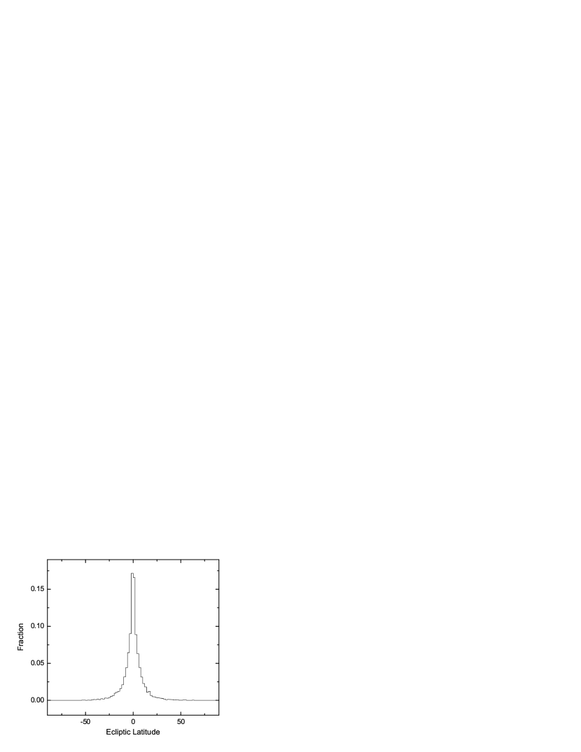
Figure 6: Ecliptic latitude distribution of Earth-impacting asteroids with $V<22.7$ twenty years before impact.

Twenty years before impact 962 objects ($\sim$9.6%) lie within the sweet spot region that encompasses topocentric solar elongations from $60\hbox{${}^{\circ}$}$ to $90\hbox{${}^{\circ}$}$. Of these, 552 ($\sim$5.5%) have an ecliptic latitude ($\beta$) in the range $-10\hbox{${}^{\circ}$}\leq\beta\leq+10\hbox{${}^{\circ}$}$ and 826 ($\sim$8.3%) have $|\beta|<20\hbox{${}^{\circ}$}$. The distribution in ecliptic latitude (Fig. 6) is distinctly broader than provided by Chesley & Spahr (2004) who showed cumulative detections made by a simulated version of the LINEAR survey (Stokes et al., 2000). The broad distribution in ecliptic latitude suggests that there is merit in extending searches for PHOs in the sweet spots to ecliptic latitudes of $\pm 20^{\circ}$. Since the southern parts of these extended sweet spots are close to the horizon from the northern hemisphere, and the northern parts of the extended sweet spots are close to the horizon from the southern hemisphere, this in turn suggests that there is merit in conducting searches for PHOs from both hemispheres or from space (e.g.  Hildebrand et al., 2007).

The middle and bottom distributions in Fig. 5 show the location of the same sample of objects 20 years before impact but with brighter magnitude limits of $V<20.7$ and $V<18.7$. Another way to interpret these figures is that they show the detectability (for the same limiting magnitude of $V<22.7$) of $H=22$ (diameter 140 m) and $H=24$ (55 m) impactors at this particular time. The smaller objects must be closer to the Earth in order to be above the system’s limiting magnitude but this also has the effect of increasing the phase angle which further decreases the apparent magnitude. Thus, smaller objects must be closer and have smaller phase angle to be detected. While searches for larger objects are efficient in the sweet spots they should be supplemented by opposition surveys to find smaller objects. e.g. 20 years before impact 2008 TC₃ had an apparent magnitude of $V\approx 31$ with an ecliptic opposition-centered longitude of $\lambda_{opp}\approx-92^{\circ}$ and latitude of $\beta\approx 2^{\circ}$ — not detectable but in the sweet spot region.

Figures 7a-d show the development of the sky-plane distribution of impactors as a function of time before impact.

• 1 day before impact the impactors are located in two main concentrations; one centered on the opposition direction and the other centered on the Sun. The impactors are widely spread in ecliptic latitude because they are close to the Earth. About half as many impactors approach from the $\lambda_{opp}>0$ (a.m./morning) side compared to the $\lambda_{opp}<0$ (p.m./evening) side. Objects that approach from the morning side are moving more slowly around the Sun than the Earth, meaning that the Earth runs into them. They have perihelia that are well inside the Earth’s orbit, or have higher inclinations. Objects that impact on the evening side catch up with the Earth in its orbit around the Sun. They have perihelia that are closer to the Earth’s orbit, or have higher eccentricities.

• 30 days before impact, the concentration that will impact from the opposition direction has moved east and is centered close to $\lambda_{opp}=20^{\circ}$. The impactors that will approach from close to the Sun direction are also further east with some of them becoming observable in the evening sweet spot.

• 60 days before impact many of the impactors that will approach the Earth from outside the Earth’s orbit are scattered around $\lambda_{opp}=40^{\circ}$ and more of the impactors that will approach from inside the Earth’s orbit are becoming visible near the evening sweet spot. This trend continues 90 days and 120 days before impact with the outside impactors moving further east and more of the inside impactors becoming more visible in the evening sweet spot.

• More than 180 days before impact the sky plane distribution of the impactors is more complex. The observability of impactors decreases significantly because of their small solar elongations. 180 days, 1 year and 1.5 years before impact many impactors are close to the direction of the Sun or are far from the Earth. Observability improves from 2 years onwards as the distribution more closely mimics the steady state distribution of impactors in the sky.

The difficulty in observing many of the impactors in the period between 0.5 and 1.5 years before collision with the Earth is important. In the event that an impact is predicted, precision astrometry will be needed during this period to determine where and when the impact will occur so that life-saving actions can be taken if necessary.

3 Next generation sky survey impactor detection performance

Our goals in this section are to determine

• the efficiency of a next-generation sky survey at identifying Earth-impacting asteroids

• the likely warning time for impending impacts

• the reason(s) why some impactors remain undetected

• methods for discovering the impactors that are most difficult to detect

• the probability that a next-generation survey will identify an impacting object as a function of its diameter

There have been numerous efforts in the recent past to simulate the performance of individual ground and/or space-based sky surveys at detecting NEOs (e.g.  Bowell & Muinonen, 1994; Jedicke et al., 2003; Harris & Bowell,, 2004; Stokes et al., 2004; Ivezić et al., 2007; Moon et al., 2008) but only Chesley & Spahr (2004) concentrated specifically on identifying impactors and their work also simulated the performance of the last generation of asteroid surveys. As discussed above, the impactors have a different orbit distribution from the NEO or even PHO population and pose different challenges to a survey and its moving object detection system. These include some pathological cases in the distribution of synodic periods for the objects, the fact that they are infrequently close enough and above the limiting magnitude of the detection system, and that at small topocentric distance their apparent rate of motion on the sky can be very small (mimicking more distant objects) and rapidly varying due to the topocentric motion of the observer. For all these reasons, when simulating the detection of impactors it is probably not sufficient to assume that all the objects will be detected and identified as imminently hazardous. A high-fidelity simulation is required that models the entire detection process from imaging through orbit determination and hazard assessment.

The Pan-STARRS surveying mode has not yet been decided upon and, realistically, will asymptotically approach its final configuration during the first year of operation. On average, each month PS1 will survey $\pi$/2 steradians or $\sim$5,000 square degrees in an ‘opposition’ survey with an overlap between months of about $\pi$/4 steradians. The opposition fields are imaged in g, r, and i each lunation near new moon. The redder (z, y) filter observations are obtained near quadrature closer to full moon to take advantage of their reduced sensitivity to scattered moonlight. Each field will be imaged twice (15-30 minutes apart) in each filter in each month and imaged in two lunations/year due to the overlapping survey area from month to month.

We employed the Pan-STARRS Moving Object Processing System (MOPS) to process synthetic detections generated in a pseudo-realistic Pan-STARRS survey. The simulated survey covers a large region (3600 deg²) of the sky around opposition (within roughly $\pm 30\hbox{${}^{\circ}$}$ from opposition in longitude and $\pm 30\hbox{${}^{\circ}$}$ from the ecliptic) and two $\sim 600$ deg² regions in the sweet spots defined by Chesley & Spahr (2004) within $\pm 10\hbox{${}^{\circ}$}$ of the ecliptic and from about $60\hbox{${}^{\circ}$}$ to $90\hbox{${}^{\circ}$}$ solar elongation. It is essentially a solar system specific sub-set of the sky that the Pan-STARRS system is expected to cover when it becomes operational.

The survey simulator is described in detail in Jedicke et al. (2005) and Denneau et al. (2007). It incorporates a crude weather simulation and a realistic survey pattern that attempts to observe fields at high altitude and on the meridian. We use a full N-body ephemeris determination to calculate the exact (RA,Dec) of each impactor in each synthetic field and then add noise to the astrometric position according to the expected PS1 S/N-dependent astrometric error model. The photometry for each object is similarly degraded and then we make a cut at S/N=5 in order to simulate the statistical loss of detections near the system’s limiting magnitude ($V=22.7$). Each field is observed twice each night within $\sim$15 minutes to allow the formation of ‘tracklets’ — pairs of detections at nearly the same spatial location that might represent the same solar system object. Fields are re-observed 3 times per lunation (weather permitting) and tracklets are linked across nights to form ‘tracks’ that are then tested for consistency using an initial orbit determination (IOD). Detections in tracks with small astrometric residuals in the IOD are subsequently differentially corrected to obtain a final orbit. The major item that is not simulated is the effect of the camera fill-factor and this could have a major impact on the survey’s efficiency. We will estimate this effect below but the simulation is otherwise one of the highest fidelity moving object simulations ever attempted.

We anticipate that there may be concerns regarding simulating the performance of detector systems especially in the sense that the simulations tend to be optimistic compared to the actual detector. In particular, in this case we have

1. used a realistic survey scenario but it is not the survey that will eventually be implemented by PS1,

2. used a simplistic weather model,

3. used a S/N-dependent astrometric error that is more appropriate to future surveys with better catalogs (at the onset of operations PS1 will probably use the USNO-B catalog (Monet et al., 2003) which will limit absolute astrometry to worse than 0.1″),

4. not incorporated false detections,

5. used an early version of the MOPS with reduced efficiency compared to the most recent version ($\sim$80% vs. $\sim$100%),

6. not accounted for the camera fill-factor (the fraction of ‘live’ pixels on the detector compared to the footprint of the focal plane on the sky).

We think that the first three factors are relatively unimportant. The implemented survey scenario is quite good and surveys most of the sky in which solar system objects will appear. The weather model is simple but has the desired effect of disrupting the cadence of observations and sometimes eliminating lunations from consideration due to there being too many bad nights. We have also tested MOPS performance under conditions of larger astrometric uncertainty and find that it still performs well.

The fact that no false detections were used in the simulation is also unimportant. In targetted smaller simulations (e.g.  Milani et al., 2008) we tested the MOPS using a full density complement of false and synthetic asteroid detections and found no degradation in performance at the 5-$\sigma$ level. In those tests the minimum ratio of false:synthetic detections was 1:1 on the ecliptic where the density of synthetic asteroid detections is highest. Since the density of asteroids decreases rapidly with latitude the false:synthetic ratio increases dramatically toward the ecliptic poles. Still, few tracklets incorporate false detections because those detections are spatially uncorrelated (in the simulation). It is likely that real survey systems will produce correlated false detections near chip gaps, due to CCD defects, diffraction spikes, etc., and this will produce more false tracklets than our simulation. However, the false tracklets will not link to other tracklets on other days and, if they do, will not pass quality control checks on the derived orbit. Furthermore, MOPS makes use of the detection’s morphology when combining detections into tracklets - the distance between the detections must be consistent with trailing observed in the detections themselves. Indeed, we have employed MOPS to identify asteroids in real data from the CFHT telescope (Masiero et al., 2009) and from Spacewatch (e.g.  Larsen et al., 2007) with excellent performance.

The last two factors are most important. The reduced efficiency of the MOPS software used in this simulation will have a proportional effect on the number of simulated impactor discoveries - about a 20% reduction. The actual system performance will therefore be about 25% better than reported here.

On the other hand, the largest negative impact on the simulation will be the PS1 camera fill-factor. The effective camera fill-factor ($f$) is reduced by the metal lines between individual OTA cells, the gaps between the CCDs, the use of some cells for guide star acquisition, dead cells, bad cells (e.g. due to charge transfer efficiency problems or dark noise) and the removal of portions of the image by the PS1 funding agency to excise fast moving satellites. We expect the overall fill-factor due to all these effects to result in $f\sim 0.88$. As described above, for solar system discoveries we require 6 detections on 3 nights within a lunation. Thus, the impact of the fill-factor on the detection efficiency ($\epsilon$) for fast moving objects like the impactor population is simply $\epsilon=f^{6}\sim 0.46$ if the inactive area is uncorrelated on the focal plane or $\epsilon=f^{3}\sim 0.68$ if it is correlated. That is, if the first detection of an object appears on an inactive area then its second detection is also likely to appear on an inactive area in the ‘correlated’ case and unlikely to do so in the ‘uncorrelated’ case. Losing ${1\over 3}$ to ${1\over 2}$ of potential discoveries due to the fill-factor is unfortunate but the loss is mitigated for slow moving distant objects because they appear near opposition in successive lunations. PS1 has two opportunities to discover the object in each of two successive lunations so the efficiency for finding these objects will be $\gtrsim 90$%. The problem is worse for objects like NEOs and impactors that spend fewer lunations above the detection threshold.

To determine the Pan-STARRS (PS1) survey efficiency for detecting impacting asteroids as a function of time and size we divided our sample of $\sim$130,000 synthetic impactors into six independent sets that were assigned different absolute magnitudes ($H$) as shown in Table 2. We can assign any $H$ to the impactors because the Bottke NEO model assumed that the size distribution of the NEOs was independent of the orbital elements. The six selected sizes span almost two orders of magnitude in diameter. The number of objects of each size was selected to provide a good number of derived objects (after processing through MOPS) and yet not so many objects as to be prohibitively expensive in processing time. Each of these six independent sets of impactors were then run through a simulation of the PS1+MOPS system.

Figure 8 shows that the efficiency of the PS1 survey at detecting impactors increases as a function of time and impactor diameter. In just four years of PS1 operations it could identify $\sim$85% of all 1 km diameter objects that will impact the Earth in the next 100 years. Interestingly, it has a $\sim$74% chance of identifying a 1 km diameter that would impact during the 4 year time span of the survey. At first glance this is surprising since PS1 can detect a 1 km diameter asteroid at opposition at a geocentric distance of $\sim$2.67 AU. The objects should be visible long before impact in the large volume of space surveyed by the PS1 system. We will explore the reasons for the ineffectiveness of the survey at detecting these large hazardous objects below.

The impactor discovery efficiency increases nearly linearly with time for objects of 200 m diameter to $\sim$40% efficiency in just four years. While this behavior cannot increase indefinitely we estimate that after 12 years the efficiency may be $\sim$80%. This is an interesting value because the Pan-STARRS PS4 system will have 4$\times$ the collecting area of the PS1 system modelled here and thus the efficiency curve for 200 m diameter objects for PS1 corresponds to the 100 m diameter efficiency curve for PS4. Thus, during its anticipated 10 year survey mission PS4 alone may reach nearly 90% completion for objects $\geq$140 m diameter or larger that will impact in the next 100 years.

Table 2: Size frequency distribution of synthetic impactors used in the PS1 survey simulation. The conversion between diameter and absolute magnitude assumes an albedo of $p=0.14$ for NEOs (Stuart & Binzel, 2004).

diameter	absolute	number
(meters)	magnitude
1000	17.75	1193
500	19.25	3816
200	21.25	4804
100	22.75	10001
50	24.25	25001
20	26.25	85000
Total		129815

The impact warning time was defined by Chodas & Giorgini (2008) as the time between impact and when the probability of an impact on the Earth is calculated to be more than 50%. However, we believe that the experience and response to the discovery of (99942) Apophis shows that the impact awareness time for an object is considerably longer than the impact warning time. Once an object is discovered that has a non-zero probability of impact it is observed obsessively at every opportunity and impact calculations are regularly refined to monitor the impact probability. We define the impact awareness time as the period between the identification of an impactor as a PHO (MOID $<0.05$ AU) and its time of impact. As discussed above, almost all the impactors in this study have MOID $\ll 0.05$ AU long before impact.

Fig. 9 (top) shows the MOID for derived objects at discovery (when at least 3 nights of observations have been obtained in the course of a single lunation). Almost all the objects will immediately be flagged as PHOs and therefore start the impact awareness time clock. The error on the MOIDs, the difference between the MOID for the synthetic object and the MOID for the derived object, are small after just a single lunation with typical $\Delta$MOID$\sim$MOID$\sim 10^{-3}$ AU. As more observations are acquired for these objects the impact probability should monotonically increase to 100%.

Figure 10 shows the impact awareness time as a function of the impactor size. Since the synthetic impactors were designed to hit the Earth at random times over the next 100 years, and large objects can be detected long before impact, it is no surprise that the impact awareness time for large discovered synthetic objects is evenly distributed over 100 years (Figure 10 top). The apparent decrease in the fraction of 1000 m objects with larger impact awareness times is an artifact of statistics - fitting a line to the distribution shows that it is consistent with being flat at the 1-$\sigma$ level. Surprisingly, the impact awareness times for small discovered synthetic objects is also evenly distributed over 100 years (Figure 10 bottom). This is because when PS1 discovers an object and observes it on $\geq$3 nights over an $\sim 10$ day period the orbit is good enough to accurately determine the MOID and determine the impact awareness time. Of course, it may be difficult to obtain followup observations of the smallest objects to refine the orbit and the impact probability calculation.

It is important to keep in mind that Fig. 10 does not include the large spike at zero warning time due to the undiscovered objects. For example, Figure 8 shows that $\sim$60% of 200 m diameter objects remain undiscovered at the end of the four years of PS1 surveying. Thus, the most probable awareness (warning) time for the smaller objects is zero. But when they are discovered before the apparition in which they impact the warning time can be many decades. As discussed above, to be 90% effective at eliminating the risk of an unanticipated impact in the next 100 years for objects $>$140 m diameter requires a PS1-like system to survey much longer or a more powerful system like PS4 (Kaiser & the Pan-STARRS Team, 2005) or the system being developed by the LSSTC (Ivezić et al., 2007).

While it is interesting to compute the efficiency with which a next generation survey such as PS1 can find impacting asteroids the reality of the situation is that it is unlikely that any large objects are on a collision course with the Earth in the next 100 years. The expected number of detected impactors, $N(D)$, is simply the product of the efficiency, $\epsilon(D)$, for detecting impactors of diameter $D$ and the size-frequency distribution of the population, $n(D)$. The efficiency was already shown in Fig. 8 for $D>20$ m. We use Brown et al. (2002)’s determination of the annual cumulative number of objects striking the Earth’s atmosphere: $N(>D)=37(D/meters)^{-2.7}$ which implies that objects in the size range of 2008 TC₃ strike the Earth about twice per year. Fig. 11 shows that unless the Earth is extremely unlucky PS1 will not detect a large ($D>20$ m) impacting asteroid. A best case linear extrapolation of $\epsilon(D)$ to $D<20$ m using just the 20 m and 50 m diameter points suggests that the likelihood of obtaining 3 nights of detections in the discovery of even smaller impactors is extremely unlikely. The efficiency is decreasing faster with smaller diameter than the number of objects is increasing.

While it is unlikely that PS1 will single-handedly obtain enough detections to determine a pre-impact orbit, the possibility of detecting a small asteroid prior to impact (such as the impactor 2008 TC₃), or precovering the asteroid after impact using an orbit derived from the bolide trajectory, is also interesting to meteoriticists. With sufficient advance notice it would be possible to organize a ground-based team to observe the asteroid’s atmospheric entry, train space-based platforms on the impact location, and prepare for recovery of meteorites. Post-impact precovery of the object could be useful to help determine the pre-impact size of the object and to verify the pre-impact orbit determination for the bolides (e.g.  Abe, 2008).

Simulating the automated detection by PS1+MOPS of smaller impactors is difficult. At the current time MOPS operates by linking together tracklets on 3 nights taken over the course of $\sim 10$ days. With typical impact velocities of $\sim 15$ km/s the best case scenario requires that PS1+MOPS first detect the object at a distance of $\sim 13\times 10^{6}$ km (approximately 10 days before impact). At PS1’s assumed limiting magnitude of $V=22.7$ this requires that the object be $>~{}3$m in diameter. Even if this situation were to unfold, variations in the object’s apparent position and velocity on the sky due to the topocentric motion of the observatory would likely render the object difficult to link within the MOPS (though we have not yet studied this scenario in detail). Instead, we consider the possibility that PS1 will detect an impacting asteroid prior to impact but on too few nights to determine a pre-impact orbit.

It is unlikely that the smallest objects ($<20$ m diameter) will be discovered, and have good enough derived orbits to guarantee impact, in any apparition except for the one in which they strike the Earth. Thus, we determined the sky-plane distribution and rate of motion 1, 5 and 10 days before impact for all the objects in Table 2.

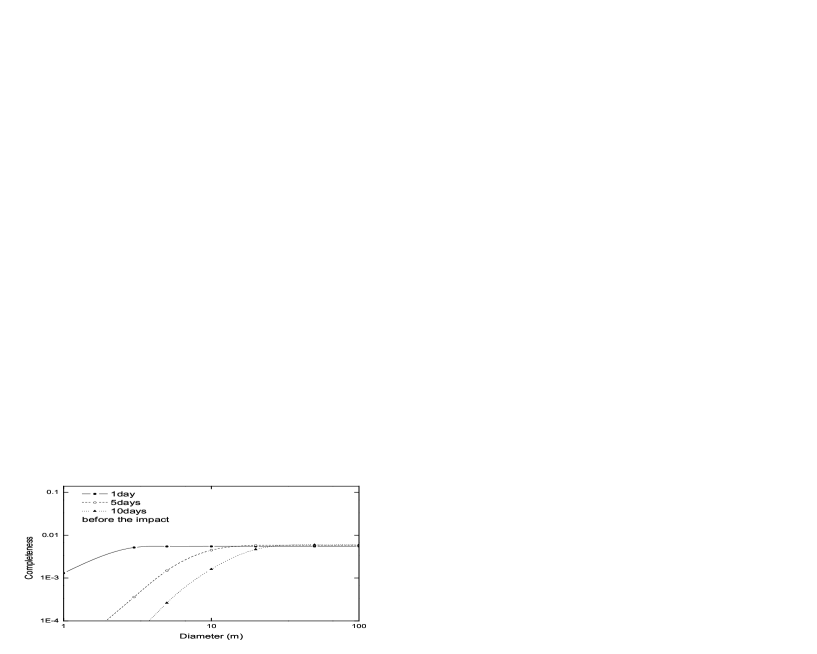
Figure 12: Estimated four year PS1 survey detection efficiency 1, 5, and 10 days before impact for small impactors on their final approach to the Earth.

Once again, since the Bottke NEO model’s orbit distribution is independent of size, and assuming that we can extend the orbit distribution of the large objects down to 1 m diameter (we have already discussed that while there is reason to believe that the Yarkovsky effect will modify the orbit distribution there is as of yet no debiased orbit distribution for the small impactors), we can assign any size or $H$ to the objects and quickly determine the ensemble’s apparent magnitude distribution. The efficiency for detecting these objects is then simply the ratio between the number that meet all our search criteria (within the surveying region, $V<22.7$, assuming that surveying takes place on only 75% of nights due to weather, and with a rate of motion within the detectability range) and the total number. Fig. 12 shows that the maximum efficiency for the smallest objects is about 0.6%.

The distributions of the rates of motion of the meteoroids before impact are shown in Fig. 13. Typical rates of motion are much slower on the final approach trajectory than on fly-by apparitions. The detectable rates of motion are limited to $0\leq\omega\leq 12$ deg/day where the upper limit is enforced by the Pan-STARRS funding agency. The figure shows clearly that the restricted rate of motion does not have a strong effect on detection efficiency when the impactors are on their approach to the Earth.

In the discussion above and elsewhere in this work we have ignored the effects of trailing loss — when objects move during the exposure time they leave ‘trails’ on the image rather than point sources and the trails have, in the past, been more difficult to identify than point sources. While the PS1 point source detection limit is expected to be $V\sim 22.7$ the efficiency of our faint trail detection algorithm is not yet known. It is thought that it should be efficient to per-pixel $S/N\ll 1$ implying that the detection efficiency could be quite good even for intrinsically faint objects. Since we have not yet measured the trailing losses we ignore them. This means that the small impactor detection efficiencies reported here and in Fig. 12 are upper limits.

Figure 11 shows the expected number of detections of small impactors (bolides) within 10 days of impact during the 4 year PS1 survey as a function of diameter using the Brown et al. (2002) size-frequency distribution (SFD). The cumulative probability of PS1 detecting a bolide in the 1-10 m size range is $25\pm 15$% (the error is determined from the SFD only). In other words, PS1 has $\sim 25$% probability of detecting another 2008 TC₃-like object during its four year survey mission.

Considering that we have argued that PS1 is the first of the next generation sky-surveys and that this powerful system only has a $\sim 25$% probability of detecting another 2008 TC₃-like object in four surveying years, how could a ‘last-generation’ survey like CSS have discovered 2008 TC₃? In addition to the impactor, the CSS has also discovered several other small asteroids making very close approaches to the Earth (e.g. 2008 UA₂₀₂). The CSS’s telescope system has (Ed Beshore, personal communication) a smaller etendue (1.5 m $\times$ 1 deg²) than the PS1 system (1.8 m $\times$ 7 deg²) at a significantly worse site (CSS FWHM $\sim 2\arcsec$ vs $\sim 1\arcsec$ for PS1; worse weather conditions; brighter sky), and twice the camera readout time ($\sim 12$ s vs. $\sim 6$s). Thus, we conservatively estimate that the PS1 system will be $\sim 10\times$ more efficient than the CSS. The CSS survey strategy sacrifices limiting magnitude to cover as much sky as possible (T. Spahr, personal communication) — an old recipe for finding more NEOs (Bowell & Muinonen, 1994). The result is that the CSS 1.5 m telescope covers about 3600 deg² per lunation to $V\sim 21$ mag while our PS1 simulation covers $\sim$3800 deg² to a limiting magnitude of $V\sim 22.7$. Based on these arguments our simulations suggest that the CSS made a low-probability discovery of 2008 TC₃ — they were lucky. Another alternative is that the SFD of the bolides from Brown et al. (2002) is in error — we consider this to be unlikely because of other corroborating research (e.g.  Ivanov, 2006).

Like the CSS discovery of 2008 TC₃, the problem is that PS1 will detect the object on only a single night resulting in an orbit with large uncertainties. PS1 can report single night detection pairs to the Minor Planet Center (MPC) but will then depend on rapid announcement by the MPC of likely impactors and prompt followup by other observatories around the world.

We have considered the possibility that detections in the impactor’s tracklet could provide information to flag it as an imminent impactor based on rapid changes in the detections’ trail length or orientation due to the effects of topocentric parallax. While the 15-30 min time difference between the detections in the tracklets probably does not provide enough leverage to make this method viable for Pan-STARRS it could be employed in the future by a dedicated impactor survey.

Since ground-based all-sky bolide impact monitoring networks (e.g.  Oberst, 1998; Weryk, 2008; Bland, 2008) cover an extremely small fraction of the Earth’s surface ($\sim$1%; P. Brown, personal communication) it is exceedingly unlikely that an object imaged by PS1 will also be detected by a ground-based sensor. On the other hand, the detection of bolides from wide-coverage space-based systems (e.g.  Koschny et al., 2004) is possible and may provide an opportunity to search through PS1 detections for pre-impact observations.

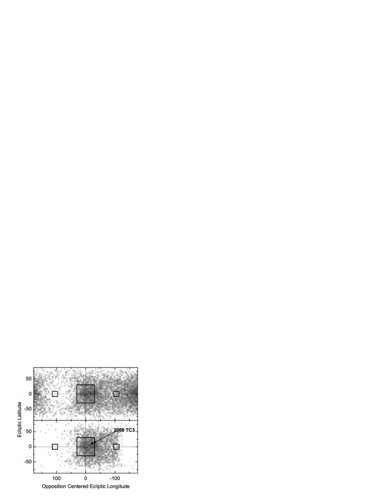
Figure 14: (top) Sky-plane probability distribution for 3 m diameter impactors (bolides) 1 day before impact with no restrictions on brightness and apparent motion. (bottom) Same as above but with $V<22.7$ and apparent motion $<12$ deg/day. Approximate PS1 search regions are shown as solid rectangles (the opposition region is in the center and the sweet spots are on the left and right). The position of 2008 TC₃ at discovery by the Catalina Sky Survey is highlighted.

Figure 14 shows the apparent sky-plane distribution for 3 m diameter bolides 1 day before impact. These small objects (e.g.  1-20 m) are visible for only a short time before impact and their apparent brightness is strongly affected by the phase angle so that they can only be detected near opposition. The location of 2008 TC₃ 3 days before impact is clearly within the PS1 opposition field. PS1 would have detected 2008 TC₃ since it was brighter than V=22.7 mag (assuming $H=30.4$ and $G=0.15$) for 4–5 days before impact (with $V=18.9$ mag at discovery  1 day before the impact) and the sky-plane motion was below the PS1 trailing cut-off of 12^∘/day.

Although the small impactors may be located over the entire sky there are two prominent clumps in Fig. 14 — towards the Sun and around the opposition point (the anti-solar direction). This result is consistent with the helion and antihelion sources (Poole, 1997) of sporadic background bolides that are the result of the velocity vector summation of the Earth and the sporadic meteors. Jones & Brown (1993) had earlier suggested that these two sources of sporadic meteors were most consistent with a population of small meteoroids derived from a Jupiter Family Comet (JFC) parent population. We note that their study did not correct for strong selection effects in the radar detection of the meteors that would favor the high velocity cometary sub-component of the helion and anti-helion sources. Considering that the Bottke NEO model employed here is dominated by asteroids but still produces these two sources it suggests that at least some component of the sporadic meteors in the helion and anti-helion regions may be of asteroidal origin.

We believe that our results encourage optimism that the suite of next generation ground-based sky surveys will be able to eliminate $\geq$90% of the risk of an unanticipated impact of an object $>140$ m diameter. Still, it is interesting to identify a survey strategy that could reduce the risk even further. Figure 15 shows that the undiscovered large (1 km) impactors rarely appear in the PS1 survey regions and are strongly clustered in the direction towards the Sun. This is not because the objects are on orbits interior to the Earth’s orbit (e.g.  Zavodny et al., 2008) but is due to their orbital period being close to one year. The synodic period with respect to Earth $P_{syn}=|P_{Earth}^{-1}-P_{asteroid}^{-1}|^{-1}$ is thus long. The four year PS1 survey has a low efficiency for detecting objects with long synodic periods and the solution is to survey over a longer time period or to survey the sky at smaller solar elongations. The suite of next generation surveys (e.g. , Pan-STARRS, LSSTC) will survey the sky for about a decade and will increase the completion statistics at all impactor sizes. Surveying closer to the Sun is realistic only from future space-based platforms (e.g.  Tedesco et al., 2000; Jedicke et al., 2003; Hildebrand et al., 2007; Mottola, 2008).

Figure 16 shows the orbital period for 1 km diameter impactors that strike the Earth during the 4 year survey mission. The orbital period of the undetected impactors peaks at 1 year as explained above. At first glance it may be surprising that a powerful survey system could miss these large impactors given the large distance at which 1 km diameter objects can be detected. The explanation is that all the undetected large impactors strike the Earth in the first 2 years; before the survey had sufficient time to explore the entire volume of the solar system to the distance at which 1 km diameter objects are detectable.

4 Conclusions/Discussion

We have used a synthetic population of Earth-impacting asteroids to determine their sky-plane distribution and detectability with one of the next generation all-sky surveys, PS1.

We find that

• while the steady state sky plane distribution of the impactors is concentrated towards small solar elongation as shown by Chesley & Spahr (2004) their sky-plane distribution exhibits interesting behavior in the couple years leading up to impact. This behavior could be exploited to identify these objects well in advance of impact.

• the requirement that a PHO have a MOID$<$0.05 AU identifies 98% of all impactors even 100 years in advance of impact. The remaining 2% have much larger MOID and the error on the MOID will not identify these objects as potential impactors since they become PHOs only after encounter with another solar system object, usually Jupiter. However, numerical exploration of their orbit evolution as routinely performed by impact monitoring sites will generally reveal these hazardous objects long before impact.

• the MOIDs determined for objects with detections obtained during just a single lunation are very good

• the impactor model that we have developed is probably a good proxy for the unbiased orbit distribution of the large bolide population based on 1) the good agreement between the impactor orbit distribution and the orbit elements for impacting asteroid 2008 TC₃ and 2) its sky-plane location at the time of discovery.

• the next generation of all-sky surveys will identify a large fraction ($\gtrsim 90$%) of impactors $>$140 m diameter in a decade-long survey designed to find them.

• the impact awareness time before impact can be many decades for impactors of any size as long as they are discovered before impact. The most likely impact awareness time for smaller impactors is zero.

• the next generation surveys will probably image a small impactor before impact but it will likely be observed over too short a time span (e.g. one night) to allow either an accurate pre-impact orbit to be computed or its identification as an imminent impactor.

• a search for pre-impact detections of a bolide is possible

• the most difficult objects to discover are those with long synodic periods relative to the Earth.

• next generation surveys like PS1 will be efficient at detecting large impactors when their impact time is more than about 2 years after the start of the survey.

Figure 1: Semi-major axis (top), eccentricity (middle) and inclination (bottom) distribution for (solid) our synthetic impactor population, (dotted) sporadic background fireballs and (dashed) the Bottke NEO model. The semi-major axis distribution is not shown beyond 5.1 AU but these data are included in the eccentricity and inclination distributions. The corresponding orbital elements for 2008 TC3 are indicated by the solid vertical line in each figure.

Figure 3: The probability that an Earth-impacting asteroid will not be identified as a PHO (MOID$>0.05AU$) as a function of time before impact. The superimposed line is a fit ($R^{2}=0.99$) to an empirically defined function: $p=1.3\times 10^{-4}+t^{0.92}$.

Figure 4: (top) The constant ($f^{\prime}$) in a fit ($\log f=\log f^{\prime}+m\log[MOID/(10^{-4}AU)]$ with $f<0.9$) to the cumulative fraction ($f$) of impactors with MOID as a function of time before impact from Figure 2. i.e. $f^{\prime}$ is the cumulative fraction of objects with MOID$\leq 10^{-4}$ AU at each of the specified time steps. The superimposed solid line is a fit ($R^{2}=0.954$) to an empirically defined function: $\log f^{\prime}=a[\log^{2}(t/days)-\log^{2}(t_{0}/days)]$ with $t$ being the time before impact, $a=-0.079$ and $t_{0}=72.8$ days. (bottom) The most probable MOID (mode) for the impactors as a function of time before impact. The superimposed solid line is a fit ($R^{2}=0.90$) to an empirically defined function: MOID (AU)$=-0.014-1.5\times 10^{-3}\ln{[((t/days)+10^{5})]}$. The Earth capture radius is shown for the highest (max ECR), most probable (mode ECR) and lowest (min ECR) encounter velocity for the impactors.

Figure 5: Topocentric opposition centered ecliptic sky plane distribution of $H=20$ ($\sim$350 m diameter) Earth-impacting asteroids 20 years before impact for a survey with a limiting magnitude of (top) $V=22.7$ (middle) $V=20.7$ and (bottom) $V=18.7$. This is sufficiently in advance of impact to represent the impactors’s steady-state sky plane distribution.

Figure 7: a) Topocentric opposition centered ecliptic sky plane distribution of Earth-impacting asteroids with $V\leq 22.7$ (top) 1 day, (middle) 30 days, and (bottom) 60 days before impact.

Figure 7: b) The opposition centered ecliptic sky plane distribution of Earth-impacting asteroids with $V\leq 22.7$ (top) 90 days, (middle) 120 days, and (bottom) 150 days before impact.

Figure 7: c) The opposition centered ecliptic sky plane distribution of Earth-impacting asteroids with $V\leq 22.7$ (top) 180 days, (middle) 1 year, and (bottom) 1.5 years before impact.

Figure 7: d) The opposition centered ecliptic sky plane distribution of Earth-impacting asteroids with $V\leq 22.7$ 2 years before impact.

Figure 8: (left) PS1 survey completeness (efficiency) as a function of time for different size impactors assuming an albedo of $0.14$. The percentages on the right side of the figure adjacent to the efficiency curves are the efficiency for detecting an impactor that strikes the Earth during the 4 year survey. (right) The efficiency for discovering objects impacting during the 4 year survey as a function of impactor diameter. A linear extrapolation to $D<20$ m using the two leftmost data points is shown with a dashed line.

Figure 9: (lower-left) The distribution of the error in the MOID ($|$MOID${}_{synthetic}-$MOID${}_{derived}|$) vs. the derived MOID for impactors detected in the simulation. (right) Distribution of the error in the MOID. (top) Distribution of the derived MOID.

Figure 10: Distribution of impact awareness times (defined in the text) for discovered synthetic impactors of different sizes. Note that the awareness time is zero for undiscovered impactors and they are not included in this figure.

Figure 11: (solid) Expected number of detections of large ($>20$ m diameter) impactors that will strike the Earth in the next 100 years that are observed 3 nights in a single lunation during a four year PS1 survey and (dashed) the number of small (1-20 m diameter) impactors detected by the PS1 system in the lunation prior to impact. The probable size range of the impacting asteroid 2008 TC₃ is indicated by the shaded region.

Figure 13: Distributions of the apparent rate of motion for small impactors 1, 5, and 10 days before impact. There is no restriction on apparent magnitude. The upper limit on the detectable rate of motion imposed by the Pan-STARRS funding agency is 12 deg/day.

Figure 15: (top) Sky-plane position probability distribution for 1 km diameter impactors that were not discovered during the simulated 4 year PS1 survey mission with no restriction on the apparent magnitude. Darker regions represent where the objects are most likely to be found. (bottom) Same as above but imposing a PS1 limiting magnitude cutoff at $V=22.7$. Approximate PS1 search regions are shown as solid rectangles.

Figure 16: Orbital period distribution for found (dotted) and undetected (solid) 1 km diameter impactors during the 4 year PS1 survey mission.

References

- Abe (2008) Abe, S. 2008. Meteoroids and Meteors - Observations and Connection to Parent Bodies. In (Eds. Mann, I., Nakamura, A. and Mukai, T.) Small Bodies in Planetary Systems, Lect. Notes Phys. 758.
- Astronomy and Astrophysics Survey Committee (2001) Astronomy and Astrophysics Survey Committee, Board on Physics and Astronomy, Space Studies Board, and National Research Council 2001. Astronomy and Astrophysics in the New Millennium. National Academy Press.
- Bland (2008) Bland, P.A., Spurný, P., Shrbený, L., Borovička, J., Bevan, A.W.R., Towner, M.C., McClafferty, T., Vaughan, D., Deacon, G., 2008. The Desert Fireball Network: First Results of Two Years Systematic Monitoring of Fireballs over the Nullarbor Desert of South Western Australia. Asteroids, Comets, Meteors conference, held in Baltimore, July 14 - 18, 2008, LPI Contribution No. 1405, paper id. 8246.
- Bottke et al. (1998) Bottke, W.F., Rubincam, D.P., Burns, J.A., 1998. Dynamical Evolution of Meteoroids via the Yarkovsky Effect. AAS, DPS meeting #30, #10.02, Vol. 30, p.1029.
- Bottke et al. (2000) Bottke, W.F., Jedicke, R., Morbidelli, A., Petit, J., Gladman, B., 2000. Understanding the Distribution of Near-Earth Asteroids. Science 288, 2190-2194.
- Bottke et al. (2002) Bottke, W.D., Morbidelli, A., Jedicke, R., Petit, J. ,Levison, H.F., Michel, P., Metcalfe, T.S.,2002. Debiased Orbital and Absolute Magnitude Distribution of the Near-Earth Objects. Icarus 156, 399-433.
- Bowell & Muinonen (1994) Bowell, E., Muinonen, K., 1994. Earth-crossing asteroids and comets: Groundbased search strategies. In: Gehrels, T. (Ed.), Hazards due to Comets and Asteroids, , Univ. of Arizona Press, Tucson, pp. 149-197.
- Brasser & Wiegert (2008) Brasser, R., & Wiegert, P. 2008, MNRAS, 386, 2031.
- Brown et al. (2002) Brown, P., Spalding, R.E., ReVelle, D.O., Tagliaferii, E., Worden, S.P., 2002. The flux of small near-Earth objects colliding with the Earth. Nature 420, 294-296.
- Burke et al. (2007) Burke, B.E., Tonry, J.L., Cooper, M.J., Doherty, P.E., Loomis, A.H., Young, D.J., Lind, T.A., Onaka, P., Landers, D.J., Daniels, P.J., Daneu, J.L., (2007. In: Blourke, Morley, M. (Eds.), Orthogonal transfer arrays for the Pan-STARRS gigapixel camera. Sensors, Cameras, and Systems for Scientific/Industrial Applications VIII, Proceedings of the SPIE 6501, 650107.
- Ceplecha et al. (1998) Ceplecha, Z., Borovička, J., Elford, W.G., ReVelle, D.O., Hawkes, R.L., Porubčan, V., Šimek, M., 1998. Meteor Phenomena and Bodies. Space Science Reviews 84, 327-471.
- Chesley & Milani (1999) Chesley, S., Milani, A., 1999. NEODyS: an online information system for near-Earth objects. AAS, DPS meeting #31, #28.06.
- Chesley & Spahr (2004) Chesley, S.R., Spahr T.B., 2004. Earth-impactors: orbital characteristics and warning times. In: Belton, M.J.S., Morgan, T.H., Samarashinha, N.H., Yeomans,D.K. (Eds.), Mitigation of Hazardous Comets and Asteroids, , Cambridge Univ. Press, Cambridge, pp.22-37.
- Chodas & Giorgini (2008) Chodas, P.W., Giorgini, J.D., 2008. Impact warning times for Near-Eearth asteroids. Asteroids, Comets, Meteors conference, held in Baltimore, July 14 - 18, 2008, LPI Contribution No. 1405, paper id. 8371.
- Denneau et al. (2007) Denneau, L., Kubica, J., Jedicke, R., 2007. The Pan-STARRS Moving Object Pipeline. Astron. Data Analysis Software and Systems XVI Conference Series, Vol. 376, Shaw, R.A., Bell, D.J. (Eds.), p.257.
- Drummond (1981) Drummond, J.D., 1981. A test of comet and meteor shower associations. Icarus 45, 545-553.
- Earth-impact database (2008) Earth Impact Database, 2008. http://www.unb.ca/passc/ImpactDatabase/index.html
- Farinella et al. (1998) Farinella, P., Vokrouhlicky, D., and Hartmann, W. K. 1998. Meteorite Delivery via Yarkovsky Orbital Drift. Icarus 132, 378-387.
- Gallant et al. (2006) Gallant, J., Gladman, B., and Ćuk, M. 2006. Current bombardment of the Earth-Moon system: Emphasis on cratering asymmetries. eprint arXiv:astro-ph/0608373.
- Galligan (2001) Galligan, D. P. 2001. Performance of the D-criteria in recovery of meteoroid stream orbits in a radar data set. MNRAS327, 623-628.
- Granvik et al. (2008) Granvik, M., Virtanen, J., Muinonen, K., 2008. OpenOrb: Open-Source Asterod-Orbit-Computation Software Including Statistical Orbital Ranging. Asteroids, Comets, Meteors 2008. LPI Contribution No. 1405, paper id. 8206.
- Grav et al. (2009) Grav, T., Jedicke, R., Denneau, L., Chesley, S., Holman, M.J., Spahr, T.B., 2009. The Pan-STARRS Synthetic Solar System Model: A tool for testing and efficiency determination of the Moving Object Processing System. Icarus x, xx-xx.
- Gehrels (1986) Gehrels, T., 1986. CCD Scanning. In: Lagerkvist, C.-I., Lindblad, B.A., Lundstedt, H., Rickman, H. (Eds.), Asteroids, Comets, and Meteors II, Univ. of Arizona Press, Tucson, pp. 19-20.
- Harris & Bowell, (2004) Harris, A.W., Bowell, E.L.G., 2004. LSST Solar System Survey - Cadence and Sky Coverage Requirements. Bulletin of the Am. Astron. Soc. 36, p.1530.
- Harris (2007) Harris, A.W., 2007. What Spaceguard did. Nature 453, 1178-1179.
- Harris (2008) Harris, A.W., 2008. An Update of the Population of NEAs and Impact Risk. AAS, DPS meeting #39, #50.01.
- Helin & Shoemaker (1979) Helin, E.F., Shoemaker, E.M., 1979. The Palomar planet-crossing asteroid survey, 1973-1978. Icarus 40, 321-328.
- Hildebrand et al. (2007) Hildebrand, A. R., Tedesco, E. F., Carroll, K. A., Cardinal, R. D., Matthews, J. M., Kuschnig, R., Walker, G. A. H., Gladman, B., Kaiser, N. R., Brown, P. G., Larson, S. M., Worden, S. P., Wallace, B. J., Chodas, P. W., Muinonen, K., Cheng, A., Gural, P., 2007. The Near Earth Object Surveillance Satellite (NEOSSat) Mission Enables an Efficient Space-Based Survey(NESS Project) of Interior-to-Earth-Orbit (IEO) Asteroids. 38th Lunar and Planetary Science Conference, LPI Contribution No. 1338, p. 2372.
- Ivanov (2006) Ivanov, B.A., 2006. Earth/Moon impact rate comparison: Searching constraints for lunar secondary/primary cratering proportion. Icarus 183, 504-507.
- Ivezić et al. (2007) Ivezić, Ž., Tyson, J.A., Jurić, M., Kubica, J., Connolly, A., Pierfederici, F., Harris, A.W., Bowell, E. & the LSST Collaboration, 2007. LSST: Comprehensive NEO detection, characterization, and orbits. In: Milani, A., Valsecchi, G.B., Vokrouhlický, D. (Eds.), Near Earth Objects, our Celestial Neighbors: Opportunity and Risk, IAU Symposium #236, Cambridge Univ., Cambridge, pp. 353-362.
- Jedicke et al. (2003) Jedicke, R., Morbidelli, A., Petit J., 2003. Earth and space-based NEO survey simulations: prospects for achieving the spaceguard goal. Icarus 161, 17-33.
- Jedicke et al. (2005) Jedicke, R., Denneau, L., Grav, T., Heasley, J., Kubica, J., Pan-STARRS Team, 2005. Pan-STARRS Moving Object Processing System. Bulletin of the Am. Astron. Soc. 37, p.1363.
- Jedicke et al. (2006) Jedicke, R.,Magnier, E.A., Kaiser, N., Chambers, K.C., 2006. The Next Decade of Solar System Discovery with Pan-STARRS. In: Milani, A., Valsecchi, G.B., Vokrouhlický, D. (Eds.), Proceedings IAU Symposium No. 236, Cambridge Univ. Press, Cambridge, pp.341-352.
- Jenniskens (2006) Jenniskens, P. 2006. Meteor Showers and their Parent Comets. Meteor Showers and their Parent Comets, by Peter Jenniskens, pp. . ISBN 0521853494. Cambridge, UK: Cambridge University Press, 2006..
- Jones & Brown (1993) Jones, J., & Brown, P. 1993, MNRAS, 265, 524
- Kaiser & the Pan-STARRS Team (2005) Kaiser, N., Pan-STARRS Team, 2005. The Pan-STARRS Survey Telescope Project. Bulletin of the Am. Astron. Soc. 37, p. 1409.
- Kessler et al. (1980) Kessler, D. J., Landry, P. M., Gabbard, J. R., & Moran, J. L. T. 1980, Solid Particles in the Solar System, 90, 137.
- Koehn & Bowell (1999) Koehn, B.W., Bowell, E., 1999. Enhancing the Lowell Observatory Near-Earth-Object Search, AAS, DPS meeting #31, #12.02.
- Koschny et al. (2004) Koschny, D., di Martino, M., Oberst, J., 2004. Meteor observation from space - The Smart Panoramical Optical Sensor (SPOSH). In: Triglav-Čekada, M., Trayner, C.(Eds.), Proceedings of the International Meteor Conference, International Meteor Organization, pp. 64-69.
- Larsen et al. (2007) Larsen, J. A., and 15 colleagues 2007. The Search for Distant Objects in the Solar System Using Spacewatch. AJ133, 1247-1270.
- Larson et al. (1998) Larson, S., Brownlee, J., Hergenrother, C., Spahr, T., 1998. The Catalina Sky Survey for NEOs. Bulletin of the Am. Astron. Soc. 30, p. 1037.
- Lindblad et al. (2003) Lindblad, B.A., Neslušan, L., Svoreň, J., Porubčan, V., 2003. IAU Meteor Database of photographic orbits version 2003. Earth, Moon and Planets 93, 249-260.
- Masiero et al. (2009) Masiero, J., Jedicke, R., Pravec, P., Durech, J., Gwyn, S., Denneau, L., Larsen, J., 2009. The Thousand Asteroid Light Curvey Survey. Submitted to Icarus.
- Milani et al. (2008) Milani, A., Gronchi, G. F., Farnocchia, D., Knežević, Z., Jedicke, R., Denneau, L., and Pierfederici, F. 2008. Topocentric orbit determination: Algorithms for the next generation surveys. Icarus 195, 474-492.
- Milani et al. (2005) Milani, A., Chesley, S. R., Sansaturio, M. E., Tommei, G., and Valsecchi, G. B. 2005. Nonlinear impact monitoring: line of variation searches for impactors. Icarus 173, 362-384.
- Monet et al. (2003) Monet, D. G., and 28 colleagues 2003. The USNO-B Catalog. AJ125, 984-993.
- Moon et al. (2008) Moon, H.-K., Byun, Y.-I., Raymond, S.N., Spahr. T., 2008. Realistic survey simulations for kilometer class near Earth objects. Icarus 193, 53-73.
- Morrison (1992) Morrison, D., 1992. The Spaceguard Survey: Report of the NASA International Near-Earth-Object Detection Workshop. NASA, Washington, D.C..
- Mottola (2008) Mottola, S., Börner, A., Grundmann, J. T., Hahn, G. J., Kazeminejad, B., Kührt, E., Michaelis, H., Montenegro, S., Schmitz, N., Spietz, P.,2008. AsteroidFinder: A Space-Based Search for IEOs. Asteroids, Comets, Meteors conference, held in Baltimore, July 14 - 18, 2008, LPI Contribution No. 1405, paper id. 8140.
- O’Brien & Greenberg (2005) O’Brien, D.P., Greenberg, R., 2005. The collisional and dynamical evolution of the main-belt and NEA size distributions. Icarus 178, 179-212.
- Oberst (1998) Oberst, J., Molau, S., Heinlein, D., Gritzner, C., Schindler, M., Spurný, P., Ceplecha, Z., Rendtel, J., Betlem, H., 1998. The ”European Fireball Network”: Current status and future prospects. Meteoritics & Planetary Science 33, 49-55.
- Poole (1997) Poole, L.M.G., 1997. The structure and variability of the helion and antihelion sporadic meteor sources. Monthly Notices of the Royal Astron. Soc. 290, 245-259.
- Pravdo et al. (1999) Pravdo, S.H., Rabinowitz, D.L., Helin, E.F., Lawrence, K.J., Bambery, R.J., Clark, C.C., Groom, S.L., Levin, S., Lorre, J., Shaklan, S.B., Kervin, P., Africano, J.A., Sydney, P., Soohoo, V., 1999. The Near-Earth Asteroid Tracking (NEAT) Program: an Automated System for Telescope Control, Wide-Field Imaging, and Object Detection. The Astronomical Journal 117, 1616-1633.
- Šimek (1995) Šimek, M., 1995. Diurnal and Seasonal Variations of Sporadic Meteor Parameters Summer and Winter Periods. Earth, Moon, and Planets 68, 545-553.
- Shoemaker (1983) Shoemaker, E.M., 1983. Asteroid and comet bombardment of the earth. In: Annual review of earth and planetary sciences, Volume 11, Annual Reviews Inc., Palo Alto, pp. 461-494.
- Sitarski (1968) Sitarski, G., 1968. Digital Computer Solution of the Equation of Position of a Comet on a Keplerian Orbit. Acta Astronomica 18, 197-205.
- Southworth & Hawkins (1963) Southworth, R.B., Hawkins, G.S., 1963. Statistics of meteor streams. Smithsonian Contributions to Astrophysics 7, 261-285.
- Stokes et al. (2000) Stokes, G.H., Evans, J.B., Viggh, H.E.M., Shelly, F.C., Pearce, E.C., 2000. Lincoln Near-Earth Asteroid Program (LINEAR). Icarus 148, 21-28.
- Stokes et al. (2002) Stokes, G. H., Evans, J.B., Larson, S.M., 2002. Near-Earth asteroid search programmes. In: Bottke, W., Cellino, A., Paolicchi, P., Binzel, R.P. (Eds.), Asteroid III, Univ. of Arizona Press, Tucson, pp. 45-54.
- Stokes et al. (2004) Stokes et al. 2004. http://neo.jpl.nasa.gov/neo/report.html.
- Stuart & Binzel (2004) Stuart, J.S., Binzel, R.P., 2004. Bias - corrected population, size distribution, and impact hazard for the near - Earth objects. Icarus 170, 295-311.
- Tancredi (1998) Tancredi, G. 1998, Celestial Mechanics and Dynamical Astronomy, 69, 119
- Tedesco et al. (2000) Tedesco, E.F., Muinonen K., Price S.D., 2000. Space-based infrared near-Earth asteroid survey simulation. Planetary and space science 48, 801-816.
- Valsecchi et al. (1999) Valsecchi, G.B., Jopek, T.J., Froeschle, Cl., 1999. Meteoroid stream identification: a new approach - I. Theory. MNRAS 304, 743-750.
- Weryk (2008) Weryk, R.J., Brown, P.G., Domokos, A., Edwards, W.N., Krzeminski, Z., Nudds, S.H., Welch, D.L., 2008. The Southern Ontario All-sky Meteor Camera Network. Earth, Moon, and Planets 102, 241-246.
- Zavodny et al. (2008) Zavodny, M., Jedicke, R., Beshore, E. C., Bernardi, F., and Larson, S. 2008. The orbit and size distribution of small Solar System objects orbiting the Sun interior to the Earth’s orbit. Icarus198, 284-293.