Generation of axisymmetric modes in cylindrical kinematic mean-field dynamos of VKS type

Abstract

In an attempt to understand why the dominating magnetic field observed in the von-Kármán-Sodium (VKS) dynamo experiment is axisymmetric, we investigate in the present paper the ability of mean field models to generate axisymmetric eigenmodes in cylindrical geometries. An $\alpha$-effect is added to the induction equation and we identify reasonable and necessary properties of the $\alpha$ distribution so that axisymmetric eigenmodes are generated. The parametric study is done with two different simulation codes. We find that simple distributions of $\alpha$-effect, either concentrated in the disk neighbourhood or occupying the bulk of the flow, require unrealistically large values of the parameter $\alpha$ to explain the VKS observations.

1 Introduction

Dynamo action generated by a flow of conducting fluid is the source of magnetic fields in astrophysical objects. Homogenous dynamos also have been observed in three laboratory experiments (Riga dynamo, Gailitis et al. 2000, Karlsruhe dynamo, Stieglitz and Müller 2001, Cadarache von-Kármán-Sodium (VKS) experiment, Monchaux et al. 2007). The analysis of the dynamo effect benefits from complementary approaches of scientific computing and experimental studies. Indeed, experimental fluid dynamos offer an opportunity to test numerical tools which can then be applied to natural dynamos. While the first two experimental dynamos produced results in agreement with the predictions of numerical simulations the successful Cadarache von-Kármán-Sodium experiment brought interesting unexpected features: (i) dynamo action is observed only with soft iron impellers and not with steel ones, (ii) the axisymmetric component dominates (i.e. the azimuthal mode $(m=0)$) when the dynamo action occurs.

Numerically simulating high permeability conductors embedded in conducting fluids is a challenging task and requires the development of new codes. We focus our attention in the present paper on a possible numerical answer to the second question: how can an axisymmetric magnetic field be generated?

The mode $(m=1)$ was observed as predicted from kinematic dynamo simulations in the Riga experiment using axisymmetric flows (Gailitis and Freiberg, 1980; Gailitis et al., 2004) and in the Karlsruhe experiment using an anisotropic $\alpha$-effect (Rädler et al., 2002) or simulations based on the realistic configuration considerering the 52 spin generators (Tilgner, 2002). Since numerical simulations prior to the VKS experiment (Marié et al., 2003; Ravelet et al., 2005; Stefani et al., 2006) also applied axisymmetric time averaged fluid flows, the mode $(m=1)$ was again predicted and utilized during the optimization process of the VKS impellers. (Recall that Cowling’s theorem forbids the excitation of an axisymmetric magnetic mode from an axisymmetric velocity field.)

Although the occurrence of the mode $(m=0)$ was a surprise, it does not contradict physics but rather demonstrates that the axisymmetric flow assumption is too simplistic. The counter-rotating impellers driving the VKS flow are responsible for a relatively high turbulence level compared to the first two dynamo experiments, and a large spectrum of azimuthal modes must be taken into account. This may be done in various ways. One can use the nonlinear approach (Bayliss et al., 2007), however the Reynolds number which is achievable using direct numerical simulations is thousand times smaller than the effective one, implying that turbulence is still poorly described. Alternatively, one can add some ad hoc non-axisymmetric flow modes in a kinematic code. Indeed, non-axisymmetric disturbances in terms of intermittent azimuthally drifting vortex structures have been observed in water experiments by Marié (2003) and de la Torre and Burguete (2007) but their influence on the dynamo process is unknown. A third possibility is provided by the application of a mean field model where the unresolved non-axisymmetric small scale fluctuations are parametrized by an $\alpha$-effect (Krause and Rädler, 1980). Although the mean field approach is somewhat controversial for large magnetic Reynolds numbers (see e.g. Courvoisier et al. 2006; Sur et al. 2008), it is numerically far less demanding than direct numerical simulations and allows the exploration of the parameter space more easily. This is the approach that we follow in the present study since it receives support from the second order correlation approximation (SOCA) as discussed in section § 3.2.

Assuming scale separation, the mean field approach parametrizes the induction action of unresolved small scale fluctuations via the $\alpha$-effect. Our purpose is to determine whether an $\alpha$-model can produce axisymmetric modes with realistic values of $\alpha$. Using $\left<\cdot\right>$ to denote the averaging operation and primes for unresolved quantities, the most simple $\alpha$-model states that

$$\left<\mbox{\boldmath$u^{\prime}$}\times\mbox{\boldmath$b^{\prime}$}\right>=\alpha\mbox{\boldmath$B$},$$ (1)

where $u^{\prime}$ denotes the fluctuating velocity field, $\mbox{\boldmath$b^{\prime}$}=\mu_{0}{\bf h}^{\prime}$ the fluctuating magnetic flux density or induction, ${\bf h}^{\prime}$ the fluctuating magnetic field, $\mu_{0}$ the vacuum permeability, $B$ the mean magnetic induction, and $\alpha$ the pseudo-tensor representing the $\alpha$-effect. The dynamo action is analyzed by solving the kinematic mean field induction equation

$$\frac{\partial\mbox{\boldmath$B$}}{\partial t}=\nabla\times\left(\mbox{\boldmath$u$}\times\mbox{\boldmath$B$}+\alpha\mbox{\boldmath$B$}-\eta\nabla\times\mbox{\boldmath$B$}\right)$$ (2)

where $u$ denotes a prescribed large scale velocity field and $\eta$ the magnetic diffusivity ($\eta=1/\mu_{0}\sigma$ with $\sigma$ the electric conductivity). In the kinematic approach the velocity field is given and any back-reaction of the magnetic field on the flow by the Lorentz force is ignored.

In case of a homogenous, isotropic, non-mirrorsymmetric small scale flow, the $\alpha$-tensor becomes isotropic and reduces to a scalar. The $\alpha$-effect provides an additional induction source by generating a mean current parallel to the large scale field. In general, the huge spatial extensions of astrophysical objects ensure that even a small and localized $\alpha$-effect, potentially supported by shear, is able to generate a large scale field (see for example Charbonneau 2005 for a review of current models of the solar magnetic cycle). In the VKS experiment a possible source of the $\alpha$-effect is the kinetic helicity caused by the shear between the outward driven fluid flow trapped between adjacent impeller blades and the slower moving fluid in the bulk of the container (Pétrélis et al., 2007). Unfortunately, no helicity measurements are available for this experiment and the magnitude and the spatial distribution of the corresponding $\alpha$-effect are not known. Although sign changes can occur within the domain, there are two limits for the $\alpha$ distribution. Either it is concentrated in the impeller region (Laguerre et al., 2008b, a), or it is uniformly distributed in the cylinder. We analyze these two extreme configurations in the paper.

The present work attempts to identify essential properties of the $\alpha$-effect that are necessary to generate an axisymmetric magnetic field in VKS-like settings. In the VKS experiment, the critical magnetic Reynolds number is $\rm{Rm}^{\rm{crit}}\approx 32$ using soft iron impellers, where $\rm{Rm}$ is the magnetic Reynolds number defined as usual as the ratio between the stretching and the diffusive terms (see Eq. 6 below). Kinematic simulations are applied close to the onset of dynamo action and are used for the estimation of the magnitude of the $\alpha$-effect necessary to produce the quoted dynamo threshold.

One important numerical difficulty consists of implementing realistic boundary conditions on the magnetic field between the conducting region and the vacuum. This is tackled in different ways in the two codes described in the Appendix. One code is based on the coupling of a boundary element method with a finite volume technique (FV/BEM, Giesecke et al. 2008), the other is based on the coupling of a finite element method with a Fourier approximation in the azimuthal direction (SFEMaNS, Guermond et al. 2009). The two codes are validated by comparing the results they give on identical problems.

The paper is organized as follows. In section 2, we consider a cylinder with no mean flow, the dynamo action is caused solely by an $\alpha^{2}$-effect. The simplified $\alpha$-tensor is similar to the one used in the modeling of the Karlsruhe experiment. We compare periodic and non-periodic axial boundary conditions. We validate our two independent codes by observing that they give the same results up to non-essential approximation errors. In section 3, we model the geometry and the flow pattern of the VKS experiment. The mean velocity field is obtained from water experiments. The $\alpha$-effect is investigated and the growth rates of the modes $(m=0)$ and $(m=1)$ are compared. Conclusions are proposed in section 4.

2 Axisymmetric $\alpha^{2}$-dynamos in cylinders

2.1 $\alpha$-model

We use cylindrical coordinates ($r,\,\theta,\,z$) throughout the paper. We first focus our attention on a cylindrical mean field dynamo model with vanishing mean flow $\mbox{\boldmath$u$}=0$. The $\alpha$-effect is the only source of dynamo action and provides the necessary coupling between the poloidal and toroidal fields which is essential to drive the dynamo instability. The induction equation (2) reduces to

$$\frac{\partial\mbox{\boldmath$B$}}{\partial t}=\nabla\times\left(\alpha\mbox{\boldmath$B$}-\eta\nabla\times\mbox{\boldmath$B$}\right).$$ (3)

To bound the parameter space, we consider a spatially constant but anisotropic $\alpha$-effect that we assume to be nonzero only in the annulus $R_{i}\leq r\leq R_{o}$. We choose a simplified version of the $\alpha$-effect modeling the forced helical flow realized in the Karlsruhe experiment where $\alpha$ has the following tensor form:

$$\alpha=\left(\begin{array}[]{ccc}\alpha_{0}&0&0\\ 0&\alpha_{0}&0\\ 0&0&0\end{array}\right)$$ (4)

The motivation for this approach originates from the modeling of turbulent flow structures in fast rotating spheres and planetary bodies like the Earth. Simplified spherical $\alpha^{2}$–dynamos with scalar, isotropic, $\alpha$-tensor and zero mean flow are known to exhibit properties that resemble essential characteristics of the Earth’s magnetic field like dipole dominance and reversal sequences. However, more realistic spatial distributions of the $\alpha$-effect like the anisotropic structure (4) usually generate equatorial dipole dynamos (Giesecke et al., 2005) unless anisotropic turbulent diffusivity is accounted for (Tilgner, 2004).

In the rest of section 2 we analyze the dynamo action in a cylinder of radius $R$ and vertical extension $H$. We evaluate the influence of the geometric constraints of the container (in terms of the aspect ratio $H/R$) and of the spatial distribution of the $\alpha$-effect (homogenous or concentrated in the annulus $R_{i}\leq r\leq R_{o}$) on the dynamo threshold. We define the critical dynamo number

$$C_{\alpha}^{\rm{crit}}=\displaystyle\frac{\alpha_{0}^{\rm{crit}}R}{\eta}$$ (5)

where $\alpha_{0}^{\rm{crit}}$ is the value of $\alpha_{0}$ at which dynamo action occurs.

2.2 Axisymmetric dynamos with a uniform $\alpha$ distribution

The aspect ratio of the Karlsruhe device is $H/R\approx 1$ according to the overall size of the cylindrical container. When looking for periodic solutions for magnetic fields, since $H$ would represent the half wavelength of a transverse dipole, we have to consider periodic cylinders of aspect ratio equal to two. In this case, the $\alpha$-effect is uniformly distributed in the cylinder. Using the SFEMaNS code, we have verified that $C_{\alpha}^{\rm{crit}}=4.8$ for the mode $(m=1)$. This result agrees with the Karlsruhe analytical modeling from Avalos-Zuñiga et al. (2003). The magnetic field observed in the Karlsruhe experiment was indeed perpendicular to the cylinder axis and described as an equatorial dipole. Note, that the critical dynamo number for the axisymmetric mode $(C_{\alpha}^{\rm{crit}}=7.15)$ is larger than the one for the mode $(m=1)$ explaining that the mode ($m=0$) was not observed.

We now investigate whether the axisymmetric mode can become dominant when the aspect ratio $H/R$ varies. We abandon the assumption of periodicity along the $z$-axis, and we consider the finite cylindric geometry. A uniform spatial distribution of $\alpha$ is still assumed. We compute the critical dynamo number for various aspect ratios in the range $[0.2;2.0]$. The results obtained with the hybrid FV/BEM code are reported in Figure 1. Computations done with the SFEMaNS code give almost identical results. These results have been shown (Stefani et al., 2009) to be similar to those obtained by Avalos-Zuñiga et al. (2007) applying the integral equation approach (Xu et al., 2008).

Figure 1: Critical dynamo number in dependence of the aspect ratio $H/R$ obtained from the FV/BEM algorithm. The transition between the modes $(m=0)$ and $(m=1)$ occurs at $H/R\approx 0.79$.

The main conclusion that we can draw from these computations is that the structure of the magnetic eigenmode passes from an equatorial dipole $(m=1)$ to an axial dipole $(m=0)$ as the container geometry passes from an elongated cylinder to a flat disk. The change of structure of the dominating mode is observed when the aspect ratio is about $H/R\approx 0.79$. If the aspect ratio of the Karlsruhe dynamo ($H/R\approx 0.84$ when the curved ended pipes are disregarded) had been chosen 10% smaller, an axisymmetric mode might have been produced. This would have enhanced the analogy of the model with geomagnetism. Since the experiment is now dismantled, further numerical work on this point is rather academic.

The eigenmodes associated with the modes $(m=0)$ for $H/R=0.5$ and $(m=1)$ for $H/R=2$ are shown in Fig. 2. The three panels on the left-hand side show the components of the axisymmetric magnetic field for the aspect ratio $H/R=0.5$ and the six panels on the right-hand side show the eigenmode for $H/R=2$. In the second case the geometric structure of the non-axisymmetric magnetic field is shown in two orthogonal meridional planes. Note, that as the azimuthal wavenumber passes from $(m=1)$ (right) to $(m=0)$ (left), the typical scale in the axial direction passes from $\sim 2$ for $H/R=2$ to less than 1 for $H/R=0.5$. When decreasing the aspect ratio, the geometric constraint on the axisymmetric current increases $C_{\alpha}^{\rm{crit}}$ by a factor of $2$.

Figure 2: Geometric structure of the magnetic field of the $\alpha^{2}$-dynamo in a finite cylinder with uniform $\alpha$-effect (obtained from FV/BEM approach). Left side: $H/R=0.5$, axisymmetric field at the marginal value $C_{\alpha}^{\rm{crit}}=9.8$ (from top to bottom: $B_{r},B_{\theta},B_{z}$). Right side: $H/R=2$, non-axisymmetric magnetic field in two meridional planes that differ by an angle of 90 degrees at $C_{\alpha}^{\rm{crit}}=5.3$. (from left to right: $B_{r}$, $B_{\theta}$, $B_{z}$). Solid curves denote positive values, dashed curves denote negative values.

2.3 Axisymmetric dynamos with an annular $\alpha$ distribution

We keep the aspect ratio $H/R=2$ which produces a transverse field when $\alpha$ is uniform, and we show now that axisymmetric dynamos can be obtained when the distribution of $\alpha$ is annular, i.e. $\alpha(r)\not=0$ if $r\in[R_{i},R]$ and $\alpha(r)=0$ if $r\in[0,R_{i})$. This study is inspired by unpublished analytical results of Avalos-Zuñiga and Plunian (2009) in periodic cylinders, where a change of structure of the dominating mode is observed for an annular distribution when $R_{i}/R\approx 0.7$.

We compare the critical dynamos numbers obtained in periodic and finite cylinders for the same aspect ratio $H/R=2$. We compare three cases: $R_{i}/R=0$, $0.5$, $0.8$. The results are summarized in Table 2.3. All the eigenmodes are steady at the threshold, the bifurcation is therefore of pitchfork type.

Periodic and finite cylinders of aspect ratio $H/R=2$ and different annular distributions of $\alpha$. The value $7.15^{*}$ results from unpublished data from Avalos-Zuñiga and Plunian (2009). Case Periodic Periodic Finite Finite $R_{i}/R$ $C_{\alpha}^{\rm{crit}}(m=0)$ $C_{\alpha}^{\rm{crit}}(m=1)$ $C_{\alpha}^{\rm{crit}}(m=0$) $C_{\alpha}^{\rm{crit}}(m=1)$ 0 $7.15^{*}$ 4.8 7.5 5.2 0.5 9 8 9.4 8.8 0.8 20 20.2 20.2 20.4

Table 2.3 shows that, depending on the value of $R_{i}/R$, there is a change of structure of the critical mode. In the periodic case the mode $(m=0)$ is critical when $R_{i}/R=0.8$ with $C_{\alpha}^{\rm{crit}}=20$ and the axial wavelength is $\lambda=1$. The mode $(m=1)$ is critical when $R_{i}/R=0.5$ with $C_{\alpha}^{\rm{crit}}=8$ and the axial wavelength is $\lambda=2$. The corresponding magnetic eigen-modes are shown in Figure 3. Note that, as expected, the magnetic field is concentrated in the region where $\alpha$ is nonzero.

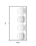
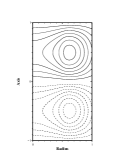
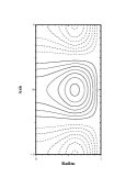
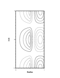
(a) (b) (c) (a’) (b’) (c’)

Figure 3: Geometric structure of the magnetic field of the $\alpha^{2}$-dynamo in a periodic cylinder of aspect ratio $H/R=2$ with an annular $\alpha$-effect: (a-c) $(m=0)$, $C_{\alpha}^{\rm{crit}}=20$ and $R_{i}/R=0.8$; (a’-c’) $(m=1)$, $C_{\alpha}^{\rm{crit}}=8$ and $R_{i}/R=0.5$. Represented are the radial (a,a’), azimuthal (b,b’) and axial (c,c’) components in the plane $\theta=0$. Data results from the SFEMaNS approach.

It is striking that the finite and the periodic results are similar when the ratio $R_{i}/R$ is nonzero (see Table 2.3 and Figure 4). The only notable effect of the top and bottom boundary conditions is to concentrate the fields inside the box. For example, the structure of the mode $(m=0)$ shown in Figure 4(a-c) is concentrated around the equator and is dominated by a quadrupolar stationary state like a ’s2t2’ state.

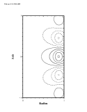
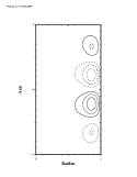
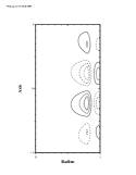
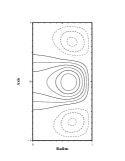
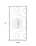
(a) (b) (c) (a’) (b’) (c’)

Figure 4: Geometric structure of the magnetic field of the $\alpha^{2}$-dynamo in a finite cylinder of aspect ratio $H/R=2$ with an annular $\alpha$-effect: (a-c) $(m=0)$, $C_{\alpha}^{\rm{crit}}=20.2$ and $R_{i}/R=0.8$ and for (a’-c’) $(m=1)$, $C_{\alpha}^{\rm{crit}}=8.8$ and $R_{i}/R=0.5$ Represented are the radial (a, a’), azimuthal (b, b’) and axial (c, c’) components. Data results from the SFEMaNS approach.

The main conclusion of this section is that axisymmetric $\alpha^{2}$-dynamos can be obtained in cylindrical geometries. In a finite cylinder with uniform distribution of $\alpha$ a dominant axisymmetric mode occurs when the aspect ratio is below the critical value $H/R\approx 0.79$. For $H/R=2$, an annular distribution of $\alpha$ can also generate an axisymmetric magnetic field if the $\alpha$-effect is sufficiently localized. Note that Tilgner (2004) obtained also an axial dipole (in a sphere) using an anisotropic magnetic diffusivity ($\eta_{\parallel}>\eta_{\perp}$). Compared to similar studies in spherical geometry, we have explored only a small region of the parameter space such as the spatial distribution of $\alpha$, its symmetry properties, and its tensor structure. This study has validated our two different codes since they obtained identical results on simple configurations. This gives us some confidence before turning our attention to the VKS experiment.

3 Mean field dynamos with a VKS type flow

3.1 Experimental setup and mean (axisymmetric) velocity field

In the von-Kármán-Sodium experiment a flow of liquid sodium is driven by two counter-rotating impellers located at the opposite ends of a cylindrical vessel. Self-generation of a magnetic field occurs if the magnetic Reynolds number exceeds the critical value ${\rm{Rm}^{\rm{crit}}}\approx 32$. It is important to note though that the dynamo is activated only when impellers made of soft iron are used. A sketch of the experimental setup is shown in Figure 5. The vessel is filled with liquid sodium. Two counter-rotating impellers are located at the endplates of the vessel each fitted with eight bended blades.

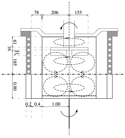
Figure 5: VKS set-up design and mean-flow structure: (upper part) dimensions and technical details of the experimental set-up, with the copper vessel including the cooling system, the thin envelope separating the flow and the stagnant liquid sodium, the impeller with fitted blades and the shaft. Courtesy of the VKS team. (lower part) Simplified geometry used in the numerical simulations in non-dimensional units. The conductivity jump between the liquid sodium and the copper vessel is taken into account. The dashed line in the lower half denotes the region where dynamo action is supported by the localized $\alpha$-effect (see section § 3.3). Note, that the simulations do not consider the region behind the impellers (lid layers).

The flow generated by the rotating blades is of von-Kármán type and has been extensively investigated in Ravelet et al. (2005). This so called s2t2-flow basically consists of two poloidal and two toroidal cells.

Throughout this paper, units are non-dimensionalized by setting the radius of the flow domain to $R=1$ (corresponding to 0.206 m in the experiment, see Fig. 5) and the magnetic diffusivity to $\eta=1$ (corresponding to $\eta_{\rm{Na}}\approx 0.1~{}{\rm{m}}^{2}/{\rm{s}}$ in the experiment). Dimensional values for the (maximum of the) velocity or the magnitude of the $\alpha$-effect are then obtained in units of ${\rm{m}}{\rm{s}}^{-1}$ by a multiplication with a factor close to $0.5$. To facilitate the dynamo action the flow region is surrounded by a layer of stagnant sodium of thickness 0.4 which is enclosed by a solid wall of copper of thickness 0.2. The fluid velocity is zero when $r>R=1$. The copper wall is modeled by a high conductivity region, i.e. $\sigma_{\rm{Cu}}\approx 4.5\sigma_{\rm{Na}}$ when $1.4\leq r\leq 1.6$. The flow is characterized by the magnetic Reynolds number

$${\rm{Rm}}=\frac{{U_{\rm{max}}R}}{\eta}$$ (6)

where $U_{\rm{max}}$ is the maximum of the fluid velocity. A typical example for a flow field realized in a water experiment in the VKS geometry is shown in Figure 6. It is time-averaged, axisymmetric and symmetrized with respect to the equator. We utilize this mean velocity field in the kinematic induction equation (2).

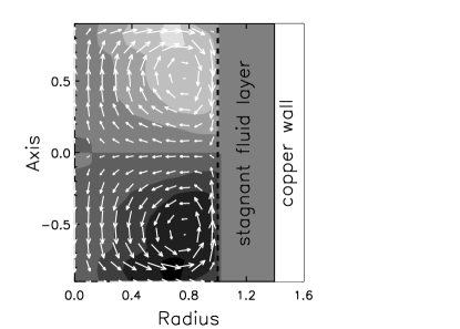
Figure 6: Axisymmetric velocity field obtained from water experiments performed by Ravelet et al. (2005) and which is applied in present kinematic simulations. Grey scale coded structures represent the azimuthal velocity field $u_{\theta}$ and the arrows represent the poloidal components ($u_{r},u_{z}$).

Using our two codes, we find that the critical Reynolds number for the mode $(m=1)$ for this setting is approximately ${\rm{Rm}}^{\rm{crit}}\approx 45$ without any $\alpha$-effect. The geometric structure of the eigenmode obtained for $\rm{Rm}=60$ is shown in Figure 7. The picture shows the iso-surface of the magnetic energy density $(2\mu_{0})^{-1}|\mbox{\boldmath$B$}|^{2}$ at 40% of the maximum value. The grey scaled map on the iso-surface represents the azimuthal component of the magnetic induction. This map shows that the mode $(m=1)$ dominates. The well known embracing banana-like structure is the dominating feature in the central region. The accumulation of magnetic energy close to the equator at the interface between the flow domain and the surrounding stagnant layer of fluid is another striking feature. Because of the equatorial symmetrization of the velocity field, the resulting eigenmode does not exhibit any azimuthal drift and remains stationary (Marié et al., 2003).

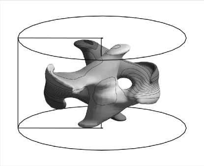
Figure 7: Iso-surface of the magnetic energy density at 40% of the maximum value. The grey scale represents the azimuthal component $B_{\theta}$.

3.2 $\alpha$-model

We now want to explore the implications of the suggestions that the strong shear between the flow trapped between the impeller blades and the slower rotating fluid neighboring the impeller results in a helical outward driven flow. The induction effects of such a flow can be parametrized by an $\alpha$-effect as illustrated in Figure 8. In this sketch an azimuthal electromotive force is produced from the cross-product of the flow $u$ between the blades and the magnetic field $b$ obtained from the distortion of an applied azimuthal magnetic field. The resulting electromotive force is parallel to the applied magnetic field but of opposite direction. This corresponds to a negative coefficient $\alpha_{\theta\theta}$ in the $\alpha$-tensor. Applying a vertical magnetic field leads to a vertical electromotive force again parallel to the applied magnetic field and of opposite direction. This corresponds to a negative coefficient $\alpha_{zz}$ in the $\alpha$-tensor.

In order to estimate the value of the coefficients $\alpha_{\theta\theta}$, $\alpha_{zz}$, we first estimate the magnetic Reynolds number of the fluid flow trapped between the impeller blades. Let $U_{\rm{disk}}$ be the rotation speed at the rim of the disc. The maximum fluid velocity is obtained just below the upper impeller and has been measured to be $U_{\rm{max}}\sim\nu U_{\rm{disk}}$ with $\nu=0.6$ denoting an impeller efficiency parameter (Ravelet et al., 2005). Then an estimate of the recirculation flow intensity is $u\sim(U_{\rm{disk}}-U_{\rm{max}})/2$. This leads to $u/U_{\rm{disk}}\sim(1-\nu)/2=0.2$. The height of a blade is $h\approx H/20\approx(1.8/20)R=0.09R$, $R$ being the disc radius and $H$ the distance between the discs. Reminding the definition of the global magnetic Reynolds number from Eq. (6), ${\rm{Rm}}=U_{\rm{max}}R/\eta\approx\nu U_{\rm{disk}}R/\eta$ we define a local magnetic Reynolds number that characterizes the flow between the blades as ${\rm{Rm}}_{\rm{blade}}\approx uh/\eta$. The combination of both definitions yields ${\rm{Rm}}_{\rm{blade}}\approx(u/U_{\rm{disk}})(h/R)({\rm{Rm}}/\nu)$ leading to ${\rm{Rm}}_{\rm{blade}}\approx 1$ for ${\rm{Rm}}\approx 32$. Therefore it seems reasonable to apply a low magnetic Reynolds number approximation to estimate the value of the $\alpha$-effect in the experiment according to the SOCA approximation (Krause and Rädler, 1980). This gives $\alpha_{\theta\theta}\sim\alpha_{zz}\sim uu_{r}h/\eta$. Assuming that the radial outward flow $u_{r}$ is of the same order as $u$, for $\eta=0.1~{}{\rm{m}}^{2}{\rm{s}}^{-1}$ and $R=0.2~{}{\rm{m}}$ we obtain $\alpha_{\theta\theta}\sim\alpha_{zz}\sim 5~{}{\rm{m}}{\rm{s}}^{-1}$. This estimate exceeds the value ($\alpha\sim 1.8~{}{\rm{m}}{\rm{s}}^{-1}$) reported by Laguerre et al. (2008b) where the efficiency factor $\nu$ was not considered in the definition of ${\rm{Rm}}$. Note, that this is only an evaluation of the order of magnitude and, as the flow is highly turbulent, the optimum value of $\alpha$ estimated above probably is not realized in the experiment.

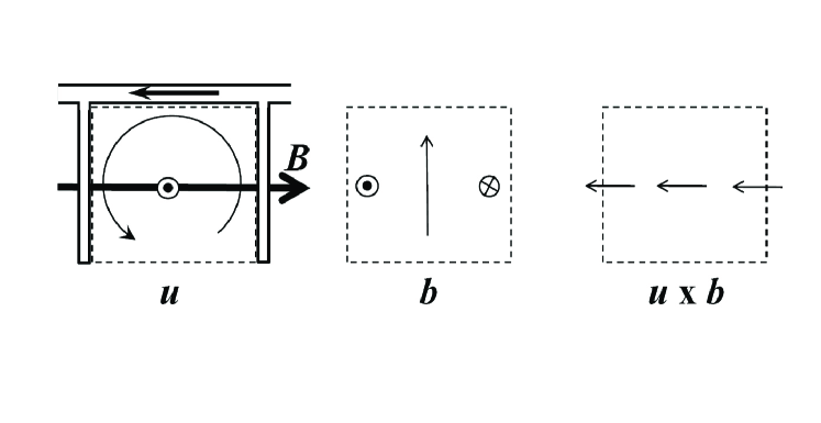
Figure 8: Sketch of the $\alpha$-model in the VKS experiment: between two impeller blades, (left) the fluid velocity (thin arrow and outwards symbol) acting on a given azimuthal mean magnetic field $B$ (thick arrow) results in a secondary magnetic field $b$ (middle) and generates an electromotive force $\mbox{\boldmath$u$}\times\mbox{\boldmath$b$}$ (right).

We henceforth focus our attention on $\alpha_{\theta\theta}$. It is indeed this coefficient that generates the poloidal component of an axisymmetric magnetic field from its toroidal component. In turn, the toroidal component is efficiently generated by twisting and stretching the poloidal field component via a shear flow ($\omega$-effect). The impact of an $\alpha_{zz}$ coefficient will be discussed at the end of the next section.

3.3 Localized $\alpha_{\theta\theta}$-effect results

As the spatial distribution of $\alpha$ is not known a priori, we start by performing simulations with the $\alpha$-effect restricted to the impeller region. More specifically we set

$$\alpha_{\theta\theta}(z)=\begin{cases}\alpha\left(1+\frac{1}{2}\left[\tanh\left(\frac{z-z_{\rm{top}}}{\Delta z}\right)-\tanh\left(\frac{z-z_{\rm{bot}}}{\Delta z}\right)\right]\right)&\text{if $0\leq r\leq R$}\\ 0&\text{if $R\leq r$}\end{cases}$$ (7)

where $\alpha$ can be positive or negative, $\Delta z=0.05$, $z_{\rm{top}}=z_{\rm{bot}}=\pm 0.8$, and $R=1$ is the radial extension of the impeller region. Equation (7) specifies a smooth transition of $\alpha_{\theta\theta}$ between a maximum value $\alpha$ in the impeller region and a vanishing value in the bulk of the container. We henceforth refer to this model as the localized $\alpha$-effect. The axial profile of $\alpha_{\theta\theta}(z)$ is shown in Figure 9.

Figure 9: Axial distribution of the localized $\alpha$-effect. The magnitude of $\alpha$ is only significant in the impeller region indicated by the dashed lines.

Figure 10 shows the growthrates of the magnetic field as a function of $\alpha$ for various magnetic Reynolds numbers.

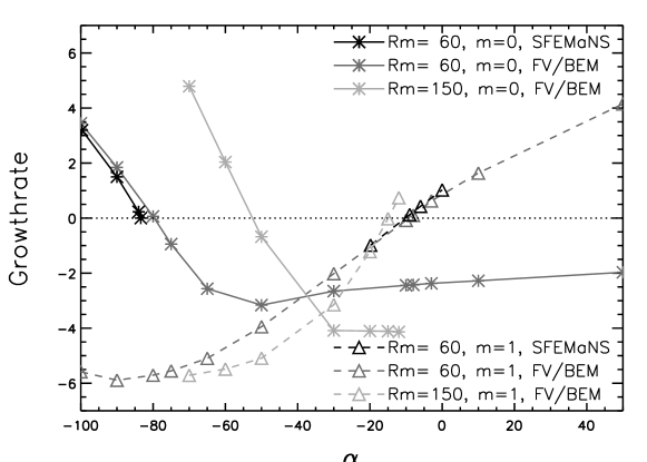
Figure 10: Field amplitude growthrates for the localized $\alpha$-effect.

The solid curves represent the growthrate for the axisymmetric mode $(m=0)$ and the dashed curves represent the results for the mode $(m=1)$. We observe two distinct dynamo regimes that differ by the resulting field geometry. The main characteristics of the dynamo solutions can be summarized as follows. For $\alpha\lesssim-50$ the eigenmode is axisymmetric whereas for $\alpha\gtrsim-15$ the mode $(m=1)$ dominates. We observe in Figure 10 that the growth rates of both modes are negative in the range $[-50,-10]$. This interval might become smaller as ${\rm{Rm}}$ increases, but it seems that there exists a non-empty range of $\alpha$ for which no dynamo action is possible at all. For instance, at $\alpha=-20$ no dynamo is obtained for ${\rm{Rm}}$ up to $300$ and the corresponding growthrates even decrease as ${\rm{Rm}}$ increases (see Figure 11).

Figure 11: Field amplitude growthrates for $\alpha=-20$ for the localized $\alpha$-distribution (7). The solid line denotes the axisymmetric mode $(m=0)$ and the dashed line denotes the mode $(m=1)$.

The existence of these two regimes becomes more obvious on Figure 12 where we show the critical magnetic Reynolds number as a function of $\alpha$. (${\rm{Rm}}^{\rm{crit}}$ is estimated by linear interpolation of two adjacent growthrates obtained close to the dynamo threshold.)

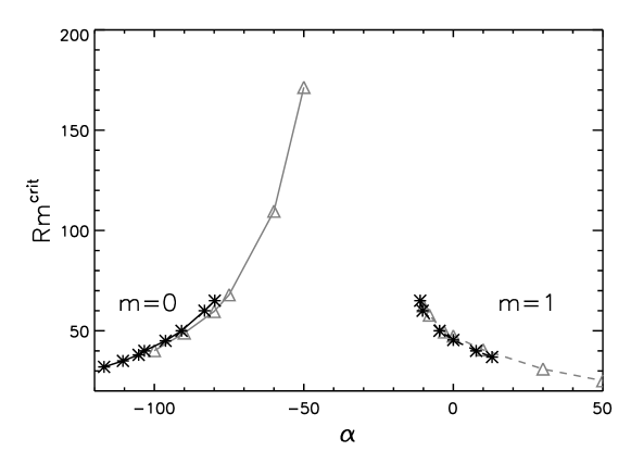
Figure 12: Critical magnetic Reynolds number in dependence of the magnitude of the $\alpha$-effect. The black curve represents the results obtained from the SFEMaNS scheme and the grey curve denotes the results of the FV/BEM approach. The left part (solid curves) shows ${\rm{Rm}}^{\rm{crit}}$ for the axisymmetric mode $(m=0)$ whereas the left part (dashed curves) is obtained for a dominating mode $(m=1)$.

The black curves represent the results provided by the SFEMaNS code and the grey curves represent the results from the FV/BEM code. Slight but systematic deviations between both codes are observed especially for large negative values of $\alpha$. Most probably the disagreement is the result of a small difference in the localization of $\alpha$ and/or the velocity field that is caused by the staggered mesh definition in the FV/BEM scheme. The present work does not intend to perform a benchmark examination of different numerical schemes so that the deviations are not investigated in detail as the general trend and the critical values of the magnetic Reynolds number are in rather good agreement.

By examination of the left branch of the graph in Figure 12 we estimate that $\alpha_{\theta\theta}\approx-115$ is necessary to obtain an axisymmetric dynamo at $\rm{Rm}\approx 32$. In physical units this value corresponds to $\alpha\approx 57.5~{}{\rm{m}}{\rm{s}}^{-1}$, which exceeds the estimated magnitude of $\alpha$ by more than a factor of $10$. Furthermore, this value is also four times larger than the maximum fluid velocity in the bulk of the cylinder. It is hard to believe that such a large $\alpha$-effect is realized in the experiment.

We performed additional simulations with an $\alpha_{zz}$ coefficient located at the impellers. The $\alpha$-tensor is therefore given by $(0,\alpha_{\theta\theta},\alpha_{zz})$ with a tanh localized function (see Eq. 7) such that ${\alpha_{\theta\theta}}=\alpha_{zz}$. We have found, for ${\rm{Rm=60}}$, $\alpha_{c}=-42.60$ with SFEMaNS and $-44.6$ with FV/BEM. These values are to be compared with $\alpha_{c}=-83.40$ for ${\rm{Rm}}=60$ obtained with a localized $(0,\alpha_{\theta\theta},0)$ $\alpha$-tensor. This reduction by a factor 2 is not enough for approaching realistic values of $\alpha$.

3.4 Uniform $\alpha$-effect results

In this section we assume that the $\alpha$-effect is uniformly distributed in the flow region ($0\leq r\leq 1,\,-0.9\leq z\leq 0.9$). Here, only the $\alpha_{\theta\theta}$ component is assumed to be nonzero.

Figure 13 shows the growthrates as a function of $\alpha$ for ${\rm{Rm}}=30,50\mbox{ and }100$. These results have been obtained with the FV/BEM code. We have verified on a few simulations (not reported here) that the SFEMaNS code produces similar results.

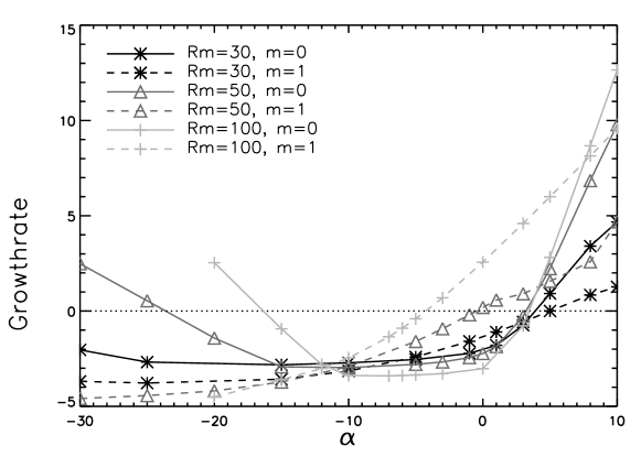
Figure 13: Field amplitude growthrates for a homogenous $\alpha$-distribution for $\rm{Rm}=30,50,100$. The solid line denotes the axisymmetric mode $(m=0)$ and the dashed line denotes the mode $(m=1)$.

We see that for large negative values of $\alpha$ the mode $(m=1)$ is suppressed in all the cases and the corresponding growthrates remain negative. The growthrate of the axisymmetric mode becomes positive for sufficiently large magnetic Reynolds numbers. Contrary to what is observed when the $\alpha$-effect is localized, positive growthrates of the axisymmetric mode are obtained for positive values of $\alpha$. For $\alpha\mathrel{\mathchoice{\vbox{\offinterlineskip\halign{\hfil$\displaystyle#$\hfil\cr>\cr\sim\cr}}}{\vbox{\offinterlineskip\halign{\hfil$\textstyle#$\hfil\cr>\cr\sim\cr}}}{\vbox{\offinterlineskip\halign{\hfil$\scriptstyle#$\hfil\cr>\cr\sim\cr}}}{\vbox{\offinterlineskip\halign{\hfil$\scriptscriptstyle#$\hfil\cr>\cr\sim\cr}}}}0$ the growthrate becomes very sensitive to small changes in $\alpha$, and a small interval exists around $\alpha\approx+5$ where the critical magnetic Reynolds number of the modes $(m=0)$ and $(m=1)$ are rather close together. This might be a promising possibility to obtain an axisymmetric field with more reasonable values for $|\alpha|$. This alternative needs to be examined in more details because positive values for $\alpha$ can be obtained in the equatorial layer where large scale intermittent vortices have been observed (Marié, 2003).

For $-15\mathrel{\mathchoice{\vbox{\offinterlineskip\halign{\hfil$\displaystyle#$\hfil\cr<\cr\sim\cr}}}{\vbox{\offinterlineskip\halign{\hfil$\textstyle#$\hfil\cr<\cr\sim\cr}}}{\vbox{\offinterlineskip\halign{\hfil$\scriptstyle#$\hfil\cr<\cr\sim\cr}}}{\vbox{\offinterlineskip\halign{\hfil$\scriptscriptstyle#$\hfil\cr<\cr\sim\cr}}}}\alpha\mathrel{\mathchoice{\vbox{\offinterlineskip\halign{\hfil$\displaystyle#$\hfil\cr<\cr\sim\cr}}}{\vbox{\offinterlineskip\halign{\hfil$\textstyle#$\hfil\cr<\cr\sim\cr}}}{\vbox{\offinterlineskip\halign{\hfil$\scriptstyle#$\hfil\cr<\cr\sim\cr}}}{\vbox{\offinterlineskip\halign{\hfil$\scriptscriptstyle#$\hfil\cr<\cr\sim\cr}}}}-7$, again, there exists a region that is characterized by an extremely high critical magnetic Reynolds number, if a dynamo could exist at all. Figure 14 shows the critical magnetic Reynolds as a function of $\alpha$ for both the localized and the uniform $\alpha$-effect. The behavior of ${\rm{Rm}}^{\rm{crit}}$ for either $\alpha$-distributions exhibits similarities like a strong tendency to diverge around a certain value of $\alpha$.

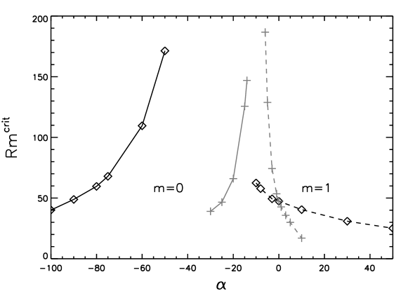
Figure 14: ${\rm{Rm}}^{\rm{crit}}$ for different $\alpha$-distributions. Black curves: localized $\alpha$-effect. Grey curves: homogenous $\alpha$-effect. Solid lines denote the results for the mode ($m=0$), dashed lines denotes the results for $m=1$.

Approximating the curves with a power law ${\rm{Rm}}^{\rm{crit}}\propto(\alpha-\alpha_{s})^{q}$ gives a diverging behavior around $\alpha_{s}\approx-18$ for the localized $\alpha$-effect and $\alpha_{s}\approx-7.4$ for the homogenous distribution.

The critical range without dynamo action becomes significantly smaller when the $\alpha$-effect is assumed to be uniform. From the negative branch ($\alpha\mathrel{\mathchoice{\vbox{\offinterlineskip\halign{\hfil$\displaystyle#$\hfil\cr<\cr\sim\cr}}}{\vbox{\offinterlineskip\halign{\hfil$\textstyle#$\hfil\cr<\cr\sim\cr}}}{\vbox{\offinterlineskip\halign{\hfil$\scriptstyle#$\hfil\cr<\cr\sim\cr}}}{\vbox{\offinterlineskip\halign{\hfil$\scriptscriptstyle#$\hfil\cr<\cr\sim\cr}}}}0$, left graphs in Figure 14) we see that when the $\alpha$ distribution is uniform, the value of $|\alpha|$ which is necessary to produce an axial dipole field at a certain $\rm{Rm}^{\rm{crit}}$ is significantly lower than when the $\alpha$-effect is localized. To obtain an axisymmetric field at ${\rm{Rm}}^{\rm{crit}}\approx 32$ we need to set $\alpha\approx-115$ when the distribution is localized and $\alpha\approx-35$ when the distribution is uniform. Comparing the volume fractions occupied by the $\alpha$-effect in both configurations (which differ by a factor of about 10), it becomes clear that the $\alpha$-effect within the impeller region operates more effectively than in the remaining active zone. However, even when the $\alpha$-effect is assumed to uniformly penetrate the entire flow domain the magnitude of $\alpha$ that is required to obtain the mode $(m=0)$ at ${\rm{Rm}}^{\rm{crit}}\approx 32$ is still $|\alpha|\approx|U_{\max}|\approx 16~{}{\rm{m}}{\rm{s}}^{-1}$ which remains unrealistic high.

4 Conclusion

The present study is an illustration in the context of the fluid dynamo problem of the interaction between numerical and experimental approaches. An account of previous stages concerning the VKS experiment may be found in Léorat and Nore (2008). We have shown that in the framework of a mean-field model, axisymmetric $\alpha^{2}$-dynamos are possible in cylinders embedded in vacuum. It seems always possible to find a configuration (either determined from geometry or by a certain spatial distribution of $\alpha$) which is able to generate an axisymmetric magnetic field.

In a VKS-like configuration, the combination of an axisymmetric flow and an $\alpha$-effect can produce axisymmetric magnetic modes as well. Our simulations with simple profiles of $\alpha$ point out however that large and unrealistic values of $\alpha$ are necessary to explain the VKS experimental results. We could think of more complex $\alpha$ distributions with negative values between the blades and positive values in the equatorial layer. This is left for future work since a realistic assessment would require to measure the kinetic helicity distribution in a water model of the VKS device.

We note also that, even if realistic values of the magnitude of the $\alpha$-effect had been obtained, one should have then to explain the non-existence of the dynamo action when using steel impellers. Indeed, at first sight, steel blades produce a flow, including kinetic helicity, close to the one driven by the soft iron blades. The role of the ferromagnetic material to obtain the dynamo action appears to be a critical issue and deserves further experimental and numerical investigations.

Appendix A Numerical methods

A.1 SFEMaNS algorithm

The SFEMaNS acronym stands for Spectral Finite Element method for Maxwell and Navier-Stokes equations. This code is designed to solve the MHD equations in axisymmetric domains in three space dimensions. To simplify the presentation we restrict ourselves in this Annex to the kinematic induction equation.

Let us consider a bounded domain $\Omega\subset\mathbb{R}^{3}$ with boundary $\Gamma=\partial\Omega$. The domain $\Omega$ is assumed to be partitioned into a conducting region (subscript $c$) and an insulating region (subscript $v$): $\overline{\Omega}=\overline{\Omega}_{c}\cup\overline{\Omega}_{v},\,{\Omega_{c}}\cap{\Omega_{v}}=\emptyset$. The interface between the conducting region and the nonconducting region is denoted by $\Sigma=\partial{\Omega_{c}}\cap\partial{\Omega_{v}}$. To easily refer to boundary conditions, we introduce ${\Gamma_{c}}=\Gamma\cap\partial{\Omega_{c}},\,{\Gamma_{v}}=\Gamma\cap\partial{\Omega_{v}}$. Note that $\Gamma={\Gamma_{v}}\cup{\Gamma_{c}}$.

A.1.1 The PDE setting

The electromagnetic field in the entire domain $\Omega={\Omega_{c}}\cup{\Omega_{v}}$ is modeled by the Maxwell equations in the MHD limit.

$$\left\{\begin{aligned} &\mu\partial_{t}{\bf H}=-\nabla{\times}{\bf E},\text{ in $\Omega$}\\ &\nabla{\times}{\bf H}=\begin{cases}\sigma({\bf E}+\mbox{\boldmath$u$}{\times}\mu{\bf H})+{\bf j}^{s},&\text{in ${\Omega_{c}}$}\cr 0,&\text{in ${\Omega_{v}}$}\end{cases}\\ &\nabla\!{\cdot}{\bf E}=0,\text{ in ${\Omega_{v}}$}\\ &{\bf E}\times{\bf n}|_{\Gamma}={\bf a},\qquad{\bf H}|_{t=0}={\bf H}_{0},\text{ in ${\Omega_{c}}$}\end{aligned}\right.$$ (8)

where ${\bf n}$ is the outward unit normal on $\Gamma$. The independent variables are space and time. The dependent variables are the magnetic field, ${\bf H}={\bf B}/\mu$, and the electric field, ${\bf E}$. The data are the initial condition, ${\bf H}_{0}$, the boundary data, ${\bf a}$, and the externally imposed distribution of current, ${\bf j}^{s}$. The data are assumed to satisfy all the usual compatibility conditions, i.e. $\nabla\!{\cdot}(\mu{\bf H}_{0})=0$. The physical parameters are the magnetic permeability, $\mu$, and the conductivity, $\sigma$. For the sake of generality, the permeabilities in each domain ($\mu^{c},\mu^{v}$) are distinguished, but we take $\mu^{c}=\mu^{v}=\mu_{0}$ in the applications considered in the paper.

A.1.2 Introduction of $\phi$ and elimination of ${\bf E}$

We assume that the initial data ${\bf H}_{0}$ is such that $\nabla{\times}{\bf H}_{0}|_{{\Omega_{v}}}=0$. We also assume that either $\Omega_{v}$ is simply connected or there is some mechanism that ensures that the circulation of ${\bf H}$ along any path in the insulating media is zero. The condition $\nabla{\times}{\bf H}|_{{\Omega_{v}}}=0$ then implies that there is a scalar potential $\phi$, defined up to an arbitrary constant, such that ${\bf H}|_{{\Omega_{v}}}=\nabla\phi$. Moreover, we can also define $\phi_{0}$ such that ${\bf H}_{0}|_{{\Omega_{v}}}=\nabla\phi_{0}$. We now define

$${\bf H}=\begin{cases}{\bf H}^{c}&\text{in ${\Omega_{c}}$}\cr\nabla\phi&\text{in ${\Omega_{v}}$},\end{cases}\qquad\mu=\begin{cases}\mu^{c}&\text{in ${\Omega_{c}}$}\cr\mu^{v}&\text{in ${\Omega_{v}}$},\end{cases}$$ (9)

and we denote ${\bf n}^{c}$ and ${\bf n}^{v}$ the outward normal on $\partial{\Omega_{c}}$ and $\partial{\Omega_{v}}$, respectively. It is possible to eliminate the electric field from the problem and we finally obtain:

$$\left\{\begin{aligned} &\mu^{c}\partial_{t}{\bf H}^{c}=-\nabla{\times}(R_{\text{\rm m}}^{-1}\sigma^{-1}(\nabla{\times}{\bf H}^{c}-{\bf j}^{s})-\mbox{\boldmath$u$}{\times}\mu^{c}{\bf H}^{c}),&&\text{in ${\Omega_{c}}$}\\ &\mu^{v}\partial_{t}{\Delta}\phi=0&&\text{in ${\Omega_{v}}$}\\ &(R_{\text{\rm m}}^{-1}\sigma^{-1}(\nabla{\times}{\bf H}^{c}-{\bf j}^{s})-\mbox{\boldmath$u$}{\times}\mu^{c}{\bf H}^{c}){\times}{\bf n}^{c}={\bf a}&&\text{on ${\Gamma_{c}}$}\\ &\mu^{v}\partial_{{{\bf n}^{v}}}(\partial_{t}\phi)=-{\bf n}^{v}{\cdot}\nabla{\times}({\bf n}^{v}{\times}{\bf a}),&&\text{on ${\Gamma_{v}}$}\\ &{\bf H}^{c}{\times}{\bf n}^{c}+\nabla\phi{\times}{\bf n}^{v}=0&&\text{on $\Sigma$}\\ &\mu^{c}{\bf H}^{c}{\cdot}{\bf n}^{c}+\mu^{v}\nabla\phi{\cdot}{\bf n}^{v}=0&&\text{on $\Sigma$}\\ &{\bf H}^{c}|_{t=0}={\bf H}^{c}_{0},\qquad\phi|_{t=0}=\phi_{0}.\end{aligned}\right.$$ (10)

A.1.3 Weak formulation

The weak formulation of (10) that we want to use has been derived in Guermond et al. (2007). We introduce the following spaces:

$${\bf L} =\{({\bf b},\varphi)\in{\bf L}^{2}({\Omega_{c}}){\times}{H^{1}_{\scriptscriptstyle\!\int\!=0}({\Omega_{v}})}\},$$ (11)

$${\bf X} =\{({\bf b},\varphi)\in{\bf H}_{\text{\rm curl}}(\Omega_{c}){\times}{H^{1}_{\scriptscriptstyle\!\int\!=0}({\Omega_{v}})};\ ({\bf b}{\times}{\bf n}^{c}+\nabla\varphi{\times}{\bf n}^{v})|_{\Sigma}=0\},$$ (12)

and we equip ${\bf L}$ and ${\bf X}$ with the norm of ${\bf L}^{2}({\Omega_{c}}){\times}H^{1}({\Omega_{v}})$ and ${\bf H}_{\text{\rm curl}}(\Omega_{c}){\times}H^{1}({\Omega_{v}})$, respectively. ${H^{1}_{\scriptscriptstyle\!\int\!=0}({\Omega_{v}})}$ is the subspace of $H^{1}({\Omega_{v}})$ composed of the functions of zero mean value. The space ${\bf H}_{\text{\rm curl}}(\Omega_{c})$ is composed of the vector-valued functions on $\Omega_{c}$ that are componentwise $L^{2}$-integrable and whose curl is also componentwise $L^{2}$-integrable.

We are now able to formulate the problem as follows: Seek the pair $({\bf H}^{c},\phi)\in L^{2}((0,+\infty);{\bf X})\cap L^{\infty}((0,+\infty);{\bf L})$ (with $\partial_{t}{\bf H}^{c}$ and $\partial_{t}\phi$ in appropriate spaces) such that for all $({\bf b},\varphi)\in{\bf X}$ and $t\in(0,+\infty)$,

$$\left\{\begin{aligned} &{\bf H}^{c}|_{t=0}={\bf H}^{c}_{0};\quad\nabla\phi|_{t=0}=\nabla\phi_{0},\\ &\int_{{\Omega_{c}}}\left[\mu^{c}(\partial_{t}{\bf H}^{c}){\cdot}{\bf b}+((R_{\text{\rm m}}\sigma)^{-1}(\nabla{\times}{\bf H}^{c}-{\bf j}^{s})-\mbox{\boldmath$u$}{\times}\mu^{c}{\bf H}^{c}){\cdot}\nabla{\times}{\bf b}\right]+\int_{{\Omega_{v}}}\mu^{v}(\partial_{t}\nabla\phi){\cdot}\nabla\varphi\\ &\hskip 56.9055pt+\int_{\Sigma}((R_{\text{\rm m}}\sigma)^{-1}(\nabla{\times}{\bf H}^{c}-{\bf j}^{s})-\mbox{\boldmath$u$}{\times}\mu^{c}{\bf H}^{c}){\cdot}({\bf b}{\times}{\bf n}^{c}+\nabla\varphi{\times}{\bf n}^{v})\\ &\hskip 56.9055pt=\int_{{\Gamma_{c}}}({\bf a}{\times}{\bf n}){\cdot}({\bf b}{\times}{\bf n})+\int_{{\Gamma_{v}}}({\bf a}{\times}{\bf n}){\cdot}(\nabla\varphi{\times}{\bf n}).\end{aligned}\right.$$ (13)

The interface integral over $\Sigma$ is zero since ${\bf b}{\times}{\bf n}^{c}+\nabla\varphi{\times}{\bf n}^{v}=0$, but we nevertheless retain it since it does not vanish when we construct the nonconforming finite element approximation in §A.1.4.

It has been shown in Guermond et al. (2007) that (13) is equivalent to (10). Observe that the boundary conditions on ${\Gamma_{v}}$ and ${\Gamma_{c}}$ in (10) are enforced naturally in (13). The interface continuity condition ${\bf H}^{c}{\times}{\bf n}^{c}+\nabla\phi{\times}{\bf n}^{v}=0$ is an essential condition, i.e. it is enforced in the space ${\bf X}$, see (12). One originality of the approximation technique introduced in Guermond et al. (2007) and recalled in §A.1.4 is to make this condition natural by using an interior penalty technique.

A.1.4 Finite element approximation

We approximate (13) by means of finite elements in the meridian section and Fourier expansions in the azimuthal direction.

The generic form of approximations of ${\bf H}^{c}$ and $\phi$ is

$$f(r,\theta,z,t)=\sum_{k=-M}^{M}f_{h}^{k}(r,z,t)e^{\text{i}k\theta},\qquad\overline{f_{h}^{k}}(r,z,t)=f_{h}^{-k}(r,z,t),\ \forall k\in\overline{0,M},$$ (14)

where $\text{i}^{2}=-1$ and $M+1$ is the maximum number of complex Fourier modes. The coefficients $f_{h}^{k}(r,z,t)$ take values in finite element spaces. We use quadratic Lagrange finite elements to approximate the Fourier components of ${\bf H}^{c}$, i.e. the three components of the magnetic field, $(H_{r}^{c},H_{\theta}^{c},H_{z}^{c})$, are continuous across the finite elements cells and are piecewise quadratic. The approximation space for the magnetic field is denoted ${\bf X}_{h}^{{\bf H}}$. Similarly, the Fourier components of the magnetic potential are approximated with quadratic Lagrange finite elements. The approximation space for the magnetic potential is denoted ${\bf X}_{h}^{\phi}$. No continuity constraint is enforced between members of ${\bf X}_{h}^{{\bf H}}$ and ${\bf X}_{h}^{\phi}$.

The Maxwell equation is approximated by using the technique introduced in Guermond et al. (2007, 2009). The main feature is that the method is non-conforming, i.e. the continuity constraint $({\bf b}{\times}{\bf n}^{c}+\nabla\varphi{\times}{\bf n}^{v})|_{\Sigma}=0$ in ${\bf X}$ (see (12)) is relaxed and enforced by means of an interior penalty method.

We use the second-order Backward Difference Formula (BDF2) to approximate the time derivatives. The nonlinear terms are made explicit and approximated using second-order extrapolation in time. Let $\Delta t$ be the time step and set $t^{n}:=n\Delta t$, $n\geq 0$. The solution to the Maxwell equation is computed by solving for ${\bf H}^{c,n+1}$ in ${\bf X}_{h}^{{\bf H}}$ and $\phi^{n+1}$ in $X_{h}^{\phi}$ so that the following holds for all ${\bf b}$ in ${\bf X}_{h}^{{\bf H}}$ and all $\varphi$ in $X_{h}^{\phi}$

$$\int_{{\Omega_{c}}}\left[\mu^{c}\frac{D{\bf H}^{c,n+1}}{\Delta t}{\cdot}{\bf b}+(R_{\text{\rm m}}\sigma)^{-1}\nabla{\times}{\bf H}^{c,n+1}{\cdot}\nabla{\times}{\bf b}\right]+\int_{{\Omega_{c}}}\mu^{v}\frac{D\phi^{n+1}}{\Delta t}{\cdot}\nabla\varphi\\ +\int_{\Sigma}((R_{\text{\rm m}}\sigma)^{-1}(\nabla{\times}{\bf H}^{c,n+1}-{\bf j}^{s})-\mbox{\boldmath$u$}{\times}\mu^{c}{\bf H}^{*}){\cdot}({\bf b}{\times}{\bf n}^{c}+\nabla\varphi{\times}{\bf n}^{v})\\ +g(({\bf H}^{c,n+1},\phi^{n+1}),({\bf b},\varphi))+s({\bf H}^{c,n+1},{\bf b})\\ =\int_{{\Omega_{c}}}(\mbox{\boldmath$u$}{\times}\mu^{c}{\bf H}^{*}+(R_{\text{\rm m}}\sigma)^{-1}{\bf j}^{s}){\cdot}\nabla{\times}{\bf b}+\int_{{\Gamma_{c}}}({\bf a}{\times}{\bf n}){\cdot}({\bf b}{\times}{\bf n})+\int_{{\Gamma_{v}}}({\bf a}{\times}{\bf n}){\cdot}(\nabla\varphi{\times}{\bf n}),$$ (15)

where we have set $D{\bf H}^{c,n+1}:=\tfrac{1}{2}(3{\bf H}^{c,n+1}-4{\bf H}^{c,n}+{\bf H}^{c,n-1})$, $D\phi^{n+1}:=\tfrac{1}{2}(3\phi^{n+1}-4\phi^{n}+\phi^{n-1})$, and

$$g(({\bf H}^{c,n+1},\phi^{n+1}),({\bf b},\varphi)) :=\beta\sum_{F\in\Sigma_{h}}h_{F}^{-1}\int_{F}({\bf H}^{c,n+1}{\times}{\bf n}^{c}+\nabla\phi^{n+1}{\times}{\bf n}^{v}){\cdot}({\bf b}{\times}{\bf n}^{c}+\nabla\varphi{\times}{\bf n}^{v}),$$ (16)

$$s({\bf H}^{c,n+1},{\bf b}) :=\gamma\int_{{\Omega_{c}}}\nabla\!{\cdot}(\mu^{c}{\bf H}^{c,n+1})\nabla\!{\cdot}(\mu^{c}{\bf b}).$$ (17)

The purpose of the bilinear form $g$ is to penalize the quantity ${\bf H}^{c,n+1}{\times}{\bf n}^{c}+\nabla\phi^{n+1}{\times}{\bf n}^{v}$ across $\Sigma$ so that it goes to zero when the mesh-size goes to zero. The coefficient $\beta$ is user-dependent. We usually take $\beta=1$. The purpose of the bilinear form $s$ is to have a control on the divergence of ${\bf H}^{c}$.

A.2 3D finite-volume/boundary-element-method (FV/BEM)

A.2.1 Finite volume method

A finite volume (FV) approach provides a robust grid based scheme for the solution of the kinematic induction equation. The local spatial discretization on a regular grid is easy to implement and allows a fast numerical solution of the induction equation in three dimensions. Physical quantities are defined at distinct locations on grid cells that are obtained from a regular subdivision of the computational domain. The components of the magnetic field ${B}_{ix,iy,iz}$ at a grid cell labeled by $(ix,iy,iz)$ are defined at the center of the cell faces and the values are interpreted as the average of the magnetic field on the specific cell face. The field update at a time step $n+1$ requires the discretization of Faraday’s law $\partial_{t}\mbox{\boldmath$B$}=-\nabla\times\mbox{\boldmath$E$}$. This implies the computation of the electric field ${E}_{ix,iy,iz}$ which is defined on the edges of a grid cell so that the localizations of the components of $E$ are slightly displaced with regard to the components of $B$. Additional computational efforts occur as the computation of $E$ requires the reconstruction of $u$ and $B$ on the edge of a grid cell. For moderate magnetic Reynolds numbers it is sufficient to apply a simple arithmetic average to interpolate $u$ and $B$ on the edge. For larger magnetic Reynolds numbers, however, more elaborate schemes have to be applied (e.g. Ziegler, 2004; Teyssier et al., 2006). The complications that arise by the definition of a second, staggered mesh are essentially outweighed by the maintenance of the divergence free condition and the conservation of the fluxes across interfaces between neighboring cells which are intrinsic properties of the specific finite volume approach.

To relax the constraints of the time step restriction an implicit solver for the diffusive part $-\nabla\times(\eta\nabla\times\mbox{\boldmath$B$})$ of the induction equation is applied. The full scheme for the semi-implicit field update at time step $n+1$ is second-order in time and is summarized by the following expression (Keppens et al., 1999):

$$\mbox{\boldmath$B$}^{n+1}=\mbox{\boldmath$B$}^{n}+\Delta tF^{\rm{exp}}\left[\mbox{\boldmath$B$}^{n}+\frac{\Delta t}{2}F[\mbox{\boldmath$B$}^{n}]\right]+\frac{\Delta t}{2}(F^{\rm{imp}}[\mbox{\boldmath$B$}^{n}]+F^{\rm{imp}}[\mbox{\boldmath$B$}^{n+1}]).$$ (18)

Here $F^{\rm{exp}}$ denotes the discretized operator accounting for the terms of the induction equation that have been made explicit ($\propto\mbox{\boldmath$u$}\times\mbox{\boldmath$B$}$ and $\alpha\mbox{\boldmath$B$}$), $F^{\rm{imp}}$ denotes the discretized operator accounting for terms made implicit ($\propto\eta\nabla\times\mbox{\boldmath$B$}$) and $F=F^{\rm{imp}}+F^{\rm{exp}}$.

A.2.2 Insulating boundary conditions

Insulating domains are characterized by a vanishing current $\mbox{\boldmath$j$}\propto\nabla\times\mbox{\boldmath$B$}=0$ so that, assuming that the vacuum domain is simply connected, $B$ can be expressed as the gradient of a scalar magnetic potential $\mbox{\boldmath$B$}=-\nabla\varPhi$. The potential $\varPhi$ is a solution to the Laplace equation

$$\Delta\varPhi=0,\quad\varPhi\rightarrow O(r^{-2})\mbox{ for }r\rightarrow\infty.$$ (19)

The computation of $B$ at the boundary requires the integration of $\Delta\varPhi~{}=~{}0$. An effective approach to compute the potential $\varPhi$ and the corresponding boundary field for insulating boundary conditions is provided by the boundary element method (BEM). This procedure has been proposed in Iskakov et al. (2004) and Iskakov and Dormy (2005), and was recently modified and applied to various dynamo problems (Giesecke et al., 2008). We now give a short description of the technique.

Consider a volume $\Omega$ that is bounded by the surface $\Gamma$ and let ${\partial}/{\partial n}=\mbox{\boldmath$n$}\cdot\nabla$ denote the outward normal derivative. After applying Green’s second theorem including some straightforward manipulations, the magnetic potential $\varPhi$ is shown to satisfy the following integral equation:

$$\frac{1}{2}\varPhi(\mbox{\boldmath$r$})=\int\limits_{\Gamma}G(\mbox{\boldmath$r$},\mbox{\boldmath$r$}^{\prime})\underbrace{\frac{\partial\varPhi(\mbox{\boldmath$r$}^{\prime})}{\partial n}}_{\displaystyle-B^{\rm{n}}(\mbox{\boldmath$r$}^{\prime})}-\varPhi(\mbox{\boldmath$r$}^{\prime})\frac{\partial G(\mbox{\boldmath$r$},\mbox{\boldmath$r$}^{\prime})}{\partial n}d\Gamma(\mbox{\boldmath$r$}^{\prime}),$$ (20)

where $G(\mbox{\boldmath$r$},\mbox{\boldmath$r$}^{\prime})$ is the Green’s function, or fundamental solution, which fulfills $\Delta G(\mbox{\boldmath$r$},\mbox{\boldmath$r$}^{\prime})=-\delta(\mbox{\boldmath$r$}-\mbox{\boldmath$r$}^{\prime})$ and is explicitly given by $G(\mbox{\boldmath$r$},\mbox{\boldmath$r$}^{\prime})=-(4\pi\left|\mbox{\boldmath$r$}-\mbox{\boldmath$r$}^{\prime}\right|)^{-1}$. $\partial_{n}\Phi=-B^{\rm{n}}$ yields the normal component of $B$ on $d\Gamma$ which is known from the finite volume method as described in the previous paragraph. The tangent components of the magnetic field $B^{\tau}$ at the boundary are computed by:

$${B}^{\tau}\!=\!\mbox{\boldmath$e$}_{\tau}\!\cdot\!\mbox{\boldmath$B$}\!=-\mbox{\boldmath$e$}_{\tau}\!\cdot\!\nabla\!\varPhi(\mbox{\boldmath$r$})\!=\!2\!\!\int\limits_{\Gamma}\!\!\mbox{\boldmath$e$}_{\tau}\!\cdot\!\left(\!\varPhi(\mbox{\boldmath$r$}^{\prime})\nabla_{r}\!\frac{\partial G(\mbox{\boldmath$r$},\mbox{\boldmath$r$}^{\prime})}{\partial n}\!+\!B^{\rm{n}}(\mbox{\boldmath$r$}^{\prime})\nabla_{r}\!G(\mbox{\boldmath$r$},\mbox{\boldmath$r$}^{\prime})\!\right)\!d\Gamma(\mbox{\boldmath$r$}^{\prime})$$ (21)

where $\mbox{\boldmath$e$}_{\tau}$ represents a tangent unit vector on the surface element $d\Gamma(\mbox{\boldmath$r$}^{\prime})$. It can been shown that Eqs. (20) and (21) contain all the contributions if all the field sources are located within the volume enclosed by $\Gamma$.

The discretization of Eq. (20) and Eq. (21) leads to an algebraic system of equations which finally determines $B^{\tau}$ at a single point on the surface by performing a matrix multiplication that connects the normal components $B^{\rm{n}}$ at every surface grid cell of the computational domain:

$$\mbox{\boldmath$B$}^{\tau}_{i}=\sum_{i=1}^{N}\mathcal{M}_{ij}\mbox{\boldmath$B$}^{\rm{n}}_{j}.$$ (22)

Eq. (22) introduces a global ordering of the quantities ${B}^{\tau}$ and $B^{\rm{n}}$ defined by an explicit mapping of the boundary grid-cell indices $(ix,iy,iz)$ on a global index $i=0,1,2,\cdots,N$ where $N=2\cdot(nz\cdot ny+nz\cdot nx+ny\cdot nx)$ represents the total number of boundary elements. The matrix elements $\mathcal{M}_{ij}$ are computed numerically applying a standard 2D-Gauss-Legendre Quadrature method. In general the matrix $\mathcal{M}$ is dense and requires a large amount of computational resources. However, $\mathcal{M}$ only depends on the geometry of the problem and therefore has only to be computed once.

References

- Avalos-Zuñiga and Plunian (2009) Avalos-Zuñiga, R. and Plunian, F., unpublished. (2009).
- Avalos-Zuñiga et al. (2003) Avalos-Zuñiga, R., Plunian, F. and Gailitis, A., Influence of electromagnetic boundary conditions onto the onset of dynamo action in laboratory experiments. Phys. Rev. E 2003, 68, 066307–+.
- Avalos-Zuñiga et al. (2007) Avalos-Zuñiga, R., Xu, M., Stefani, F., Gerbeth, G. and Plunian, F., Cylindrical anisotropic dynamos. Geophys. Astrophys. Fluid Dyn. 2007, 101, 389–404.
- Bayliss et al. (2007) Bayliss, R.A., Forest, C.B., Nornberg, M.D., Spence, E.J. and Terry, P.W., Numerical simulations of current generation and dynamo excitation in a mechanically forced turbulent flow. Phys. Rev. E 2007, 75, 026303–+.
- Charbonneau (2005) Charbonneau, P., Dynamo Models of the Solar Cycle. Living Reviews in Solar Physics 2005, 2, 2–+.
- Courvoisier et al. (2006) Courvoisier, A., Hughes, D.W. and Tobias, S.M., Effect in a Family of Chaotic Flows. Phys. Rev. Lett. 2006, 96, 034503–+.
- de la Torre and Burguete (2007) de la Torre, A. and Burguete, J., Slow Dynamics in a Turbulent von Kármán Swirling Flow. Phys. Rev. Lett. 2007, 99, 054101–+.
- Gailitis and Freiberg (1980) Gailitis, A. and Freiberg, Y., Nonuniform model of a helical dynamo. Magnetohydrodynamics 1980, 16, 11–15.
- Gailitis et al. (2000) Gailitis, A., Lielausis, O., Dement’ev, S., Platacis, E., Cifersons, A., Gerbeth, G., Gundrum, T., Stefani, F., Christen, M., Hänel, H. and Will, G., Detection of a Flow Induced Magnetic Field Eigenmode in the Riga Dynamo Facility. Phys. Rev. Lett. 2000, 84, 4365–4368.
- Gailitis et al. (2004) Gailitis, A., Lielausis, O., Platacis, E., Gerbeth, G. and Stefani, F., Riga dynamo experiment and its theoretical background. Phys. Plasmas 2004, 11, 2838–2843.
- Giesecke et al. (2005) Giesecke, A., Rüdiger, G. and Elstner, D., Oscillating -dynamos and the reversal phenomenon of the global geodynamo. Astron. Nachr. 2005, 326, 693–700.
- Giesecke et al. (2008) Giesecke, A., Stefani, F. and Gerbeth, G., Kinematic simulations of dynamo action with a hybrid boundary-element/finite-volume method. Magnetohydrodynamics 2008, 44, 237–252.
- Guermond et al. (2007) Guermond, J.L., Laguerre, R., Léorat, J. and Nore, C., An Interior Penalty Galerkin Method for the MHD equations in heterogeneous domains. J. Chem. Phys. 2007, 221, 349–369.
- Guermond et al. (2009) Guermond, J.L., Laguerre, R., Léorat, J. and Nore, C., Nonlinear magnetohydrodynamics in axisymmetric heterogeneous domains using a Fourier/Finite Element technique and an Interior Penalty Method. to appear in J. Chem. Phys. 2009.
- Iskakov and Dormy (2005) Iskakov, A. and Dormy, E., On magnetic boundary conditions for non-spectral dynamo simulations. Geophys. Astrophys. Fluid Dyn. 2005, 99, 481–492.
- Iskakov et al. (2004) Iskakov, A.B., Descombes, S. and Dormy, E., An integro-differential formulation for magnetic induction in bounded domains: boundary element-finite volume method. J. Chem. Phys. 2004, 197, 540–554.
- Keppens et al. (1999) Keppens, R., Tóth, G., Botchev, M.A. and van der Ploeg, A., Implicit and semi-implicit schemes: Algorithms. International Journal for Numerical Methods in Fluids 1999, 30, 335–352.
- Krause and Rädler (1980) Krause, F. and Rädler, K.H., Mean-field magnetohydrodynamics and dynamo theory, 1980 (Oxford: Pergamon Press).
- Laguerre et al. (2008a) Laguerre, R., Nore, C., Ribeiro, A., Léorat, J., Guermond, J.L. and Plunian, F., Erratum: Impact of Impellers on the Axisymmetric Magnetic Mode in the VKS2 Dynamo Experiment [Phys. Rev. Lett. 101, 104501 (2008)]. Phys. Rev. Lett. 2008a, 101, 219902–+.
- Laguerre et al. (2008b) Laguerre, R., Nore, C., Ribeiro, A., Léorat, J., Guermond, J.L. and Plunian, F., Impact of Impellers on the Axisymmetric Magnetic Mode in the VKS2 Dynamo Experiment. Phys. Rev. Lett. 2008b, 101, 104501–+.
- Léorat and Nore (2008) Léorat, J. and Nore, C., Interplay between experimental and numerical approaches in the fluid dynamo problem. Comptes Rendus Physique 2008, 9, 741–748.
- Marié (2003) Marié, L., Transport de moment cinétique et de champ magnétique par un écoulement tourbillonnaire turbulent : influence de la rotation. PhD thesis 2003.
- Marié et al. (2003) Marié, L., Burguete, J., Daviaud, F. and Léorat, J., Numerical study of homogeneous dynamo based on experimental von Kármán type flows. Eur. Phys. J. B 2003, 33, 469–485.
- Monchaux et al. (2007) Monchaux, R., Berhanu, M., Bourgoin, M., Moulin, M., Odier, P., Pinton, J.F., Volk, R., Fauve, S., Mordant, N., Pétrélis, F., Chiffaudel, A., Daviaud, F., Dubrulle, B., Gasquet, C., Marié, L. and Ravelet, F., Generation of a Magnetic Field by Dynamo Action in a Turbulent Flow of Liquid Sodium. Phys. Rev. Lett. 2007, 98, 044502.
- Pétrélis et al. (2007) Pétrélis, F., Mordant, N. and Fauve, S., On the magnetic fields generated by experimental dynamos. Geophys. Astrophys. Fluid Dyn. 2007, 101, 289.
- Rädler et al. (2002) Rädler, K.H., Rheinhardt, M., Apstein, E. and Fuchs, H., On the mean-field theory of the Karlsruhe Dynamo Experiment. Nonlin. Proc. in Geophys. 2002, 9, 171–187.
- Ravelet et al. (2005) Ravelet, F., Chiffaudel, A., Daviaud, F. and Léorat, J., Toward an experimental von Kármán dynamo: Numerical studies for an optimized design. Phys. Fluids 2005, 17, 117104–+.
- Stefani et al. (2009) Stefani, F., Giesecke, A. and Gerbeth, G., Numerical simulations of liquid metal experiments on cosmic magnetic fields. Theor. Comp. Fluid Dyn. 2009, submitted.
- Stefani et al. (2006) Stefani, F., Xu, M., Gerbeth, G., Ravelet, F., Chiffaudel, A., Daviaud, F. and Léorat, J., Ambivalent effects of added layers on steady kinematic dynamos in cylindrical geometry: application to the VKS experiment. Eur. J. Mech. B 2006, 25, 894–908.
- Stieglitz and Müller (2001) Stieglitz, R. and Müller, U., Experimental demonstration of a homogeneous two-scale dynamo. Phys. Fluids 2001, 13, 561–564.
- Sur et al. (2008) Sur, S., Brandenburg, A. and Subramanian, K., Kinematic -effect in isotropic turbulence simulations. MNRAS 2008, 385, L15–L19.
- Teyssier et al. (2006) Teyssier, R., Fromang, S. and Dormy, E., Kinematic dynamos using constrained transport with high order Godunov schemes and adaptive mesh refinement. J. Chem. Phys. 2006, 218, 44–67.
- Tilgner (2002) Tilgner, A., Numerical simulation of the onset of dynamo action in an experimental two-scale dynamo. Phys. Fluids 2002, 14, 4092–4094.
- Tilgner (2004) Tilgner, A., Small Scale Kinematic Dynamos: Beyond the -Effect. Geophys. Astrophys. Fluid Dyn. 2004, 98, 225–234.
- Xu et al. (2008) Xu, M., Stefani, F. and Gerbeth, G., The integral equation approach to kinematic dynamo theory and its application to dynamo experiments in cylindrical geometry. J. Chem. Phys. 2008, 227, 8130–8144.
- Ziegler (2004) Ziegler, U., A central-constrained transport scheme for ideal magnetohydrodynamics. J. Chem. Phys. 2004, 196, 393–416.