Predictive Statistical Mechanics for Glass Forming Systems

Abstract

Using two extremely different models of glass formers in two and three dimensions we demonstrate how to encode the subtle changes in the geometric rearrangement of particles during the scenario of the glass transition. We construct a statistical mechanical description that is able to explain and predict the geometric rearrangement, the temperature dependent thermodynamic functions and the $\alpha$-relaxation time within the measured temperature range and beyond. The theory is based on an up-scaling to proper variables (quasi-species) which is validated using a simple criterion. Once constructed, the theory provides an accurate predictive tool for quantities like the specific heat or the entropy at temperatures that cannot be reached by measurements. In addition, the theory identifies a rapidly increasing typical length scale $\xi$ as the temperature decreases. This growing spatial length scale determines the $\alpha$-relaxation time as $\tau_{\alpha}\sim\exp(\mu\xi/T)$ where $\mu$ is a typical chemical potential per unit length.

I Introduction

For typical glass formers with soft potentials the “glass transition” is accompanied by a dramatic increase of relaxation times: the viscosity of the super-cooled liquid shoots up by fifteen orders of magnitude within a relatively short temperature range 96EAN . When the liquid is examined on microscopic time scales, the molecules seem jammed, trapped into moving only within their cages. Of course, on the much longer viscous time scale these same systems do reach equilibrium by restructuring themselves through an ergodic exchange of particles between cages. As long as the system is ergodic it lends itself, at least in principle 08EP , to a statistical mechanical treatment. Nevertheless, it is extremely hard to reach a useful statistical mechanical theory as long as one considers the glass former on the level of its constituent particles because it is difficult to evaluate partition-function integrals in continuous coordinates. It is therefore tempting to find a reasonable up-scaling (coarse-graining) method that would define a discrete statistical-mechanics with partition sums rather than integrals, with the sum running on a finite number of quasi-species having well characterized degeneracies and enthalpies. Indeed, in a number of examples in 2-dimensions (2D) 07ABIMPS ; 07HIMPS ; 07ILLP ; 08LP ; 09LPR and in one example in 3D 09LPZ it was shown recently that such a discrete statistical-mechanics is possible and quite advantageous 08HIP ; 08HIPS in providing a successful description of the statistics and the dynamics of systems undergoing the glass transition. In this paper we examine how far the predictions of such a statistical mechanical theory can be pushed. As the theory is developed on the level of up-scaled quasi-species, one can ask whether the energy, entropy and other thermodynamic quantities appearing in the quasi-species language are identical numerically to the corresponding quantities of the system itself when computed on the level of constituting particles. One of the aims of this paper is to answer this question in the affirmative. This means that the statistical mechanical theory can be used to quantitatively predict physical observables of interest also beyond the range of measurements, hopefully providing a satisfactory understanding of the phenomenology of glass formation.

To demonstrate the generality of the approach we examine two extremely different models of glass formers to which we apply the same procedure of: i) identifying an appropriate up-scaling ii) validating that the chosen up-scaling yields a consistent statistical mechanics and iii) demonstrating how the resulting theory provides a good understanding of the subtle geometric organizational changes as a function of temperature, of the thermodynamic functions and of the relaxation time. We will stress the point that understanding the way that the concentrations of the available up-scaled quasi-species depend on the temperature is tantamount to understanding the scenario of the glass transition. To underline the generality of the approach we deal below with two models, one model is studied in 3D in an NPT ensemble and the other in 2D in an NVT ensemble. A short announcement of the results pertaining to the first model was published in 09LPZ and here we provide considerably richer details. The results of the second model are novel to the present paper. The models were chosen, as explained below, to represent extremely different microscopic characteristics; nevertheless once up-scaled, the statistical mechanics appears very similar encouraging us to propose that the approach is rather general.

The structure of the paper is as follows: in Sect. II we introduce the two models studied below, discuss the dynamics of their correlation functions as a function of temperature, and measure the relaxation time $\tau_{\alpha}$ that will be later connected to the statistical mechanical theory. In Sect. III we present the upscaling for these two models. This upscaling defines quasi-species in terms of carefully chosen groups of particles rather than individual particles. We then show how the scenario of the glass formation can be characterized by the temperature dependence of the concentrations of the various available quasi-species. Since this upscaling is not unique, we present a validation of the choice of quasi-species. The validation is a demonstration that the choice of quasi-species provides a self-consistent statistical mechanics. In other words, each quasi-species is characterized by its own enthalpy and its own degeneracy. The statistical mechanics is then shown to be able to accurately recapture the scenario of the glass formation in temperatures where data is available, and to continue to predict it for temperatures that are outside the range of numerical simulations. In Sect. IV we relate the upscaled picture to the dynamics of the system. We show how a natural static length-scale is appearing, and how this length scale characterizes the relaxation time $\tau_{\alpha}$. Finally, in Sec. V we demonstrate that the statistical mechanics as defined on the upscaled quasi-species is able to provide the correct thermodynamic function for the original system. In other words, we can compute the energy, entropy, specific heat etc. directly from the upscaled picture, in the range of temperatures accessible to simulations as well as for temperatures that are inaccessible to simulations. In Sect. VI we discuss the degree of generality of the present approach and stress what are the remaining riddles for future research.

II Two models of Glass Formation

II.1 Three-dimensional Binary Model in NPT ensemble

Some results concerning the upscaling of the first model that is studied below were announced already in 09LPZ , and here we provide further details. The model is a version of a much studied model 93KA ; 89DAY ; 99PH ; 08BPGSD , here of a 50:50 mixture of $N$ point-particles in 3-dimensions ($N=4096$ in our case), interacting via a binary potential. We refer to half the particles as ‘small’ and half as ‘large’; they interact via the potential $U(r_{ij})$:

$$U(r_{ij})=\left\{\begin{array}[]{ccl}\epsilon\left[\left(\frac{\sigma_{ij}}{r_{ij}}\right)^{\alpha}-\left(\frac{\sigma_{ij}}{r_{ij}}\right)^{\beta}+a_{0}\right]&,&r_{ij}\leq r_{c}(i,j)\\ 0&,&r_{ij}>r_{c}(i,j)\end{array}\right.$$ (1)

Here, $\epsilon$ is the energy scale and $\sigma_{ij}=1.0\sigma,1.2\sigma$ or 1.4$\sigma$ for small-small, small-large or large-large interactions, respectively. For the sake of numerical speed the potential is cut-off smoothly at a distance, denoted as $r_{c}$, which is calculated by solving $\partial U/\partial r_{ij}|_{r_{ij}=r_{c}}=0$ which translates to $r_{c}=\left({\alpha}/{\beta}\right)^{\frac{1}{\alpha-\beta}}\sigma_{ij}$. The parameter $a_{0}$ is chosen to guarantee the condition $U(r_{c})=0$. Below we use $\alpha=8$ and $\beta=6$, resulting in $r_{c}=\sqrt{8/6}~{}\sigma_{ij}$ and $a_{0}=0.10546875$, see Fig. 1. Note that the potential is purely repulsive, in a premeditated distinction from the second model discussed in Subsect. II.2

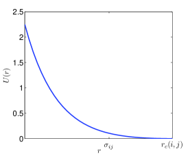
Figure 1: Color online: The pair-wise potential of the binary model

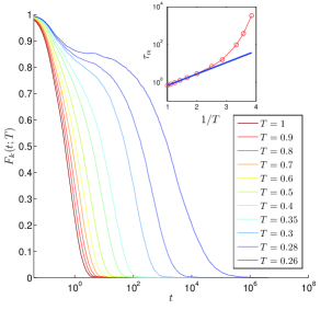
Figure 2: Color online: Time dependence of the correlation functions (2) for a range of temperatures (decreasing from left to right) as shown in the figure. The inset shows the relaxation time $\tau_{\alpha}$ in a log-lin plot vs $1/T$, compared to an Arrhenius temperature dependence.

The model dynamics were studied as a function of the temperature keeping the pressure fixed at $p=10$ (NPT ensemble). The model was simulated by employing the Verlet integration scheme with the Berendsen thermostat and barostat 91AT . The units of mass are the mass of the particles $m$, energy is measured in units of $\epsilon$ and the fundamental length scale is $\sigma$. The slowing down in the super-cooled regime is exemplified by measuring the self-part of the intermediate scattering function 99PH summed over the large particles only,

$$F_{k}(t;T)\equiv\left\langle\frac{2}{N}\sum_{i=1}^{N/2}\exp\left\{{i{\bm{k}}\cdot[{\bm{r}}_{i}(t)-{\bm{r}}_{i}(0)]}\right\}\right\rangle\ .$$ (2)

In Fig. 2 we show these correlation functions for $k=5.1\sigma^{-1}$ and for a range of temperatures as indicated in the figure. We see the usual rapid slowing down that can be measured by introducing the typical time scale $\tau_{\alpha}$ that is determined by the time where $F_{k}(t=\tau_{\alpha};T)=F_{k}(0;T)/e\equiv 1/e$. The relaxation times are shown in the inset of Fig. 2 as a function of $1/T$ in a log-lin plot to stress the non-Arrhenius dependence at lower $T$.

II.2 Two-dimensional ‘hump’ model in NVT ensemble

The second model is constructed following 89Dzu such as to have very different microscopic properties from the binary model. The interaction potential is constructed as a piecewise function consisting of the repulsive part of a standard 12-6 Lennard–Jones potential connected at $r_{0}=2^{1/6}\sigma$ to a polynomial interaction $P(x)=\sum_{i}a_{i}x^{i}$. The $a_{i}$’s are tuned so that $P(x)$ displays a peak at $r=r_{\mbox{\tiny hump}}$ and also such that there is a smooth continuity (up to second derivatives) with the Lennard–Jones interaction at $U(r_{0})=\epsilon h_{0}$ as well as with the cut-off interaction range $U(r_{\star})=0$. The interaction potential for the hump model reads:

$$U(r_{ij})=\left\{\begin{array}[]{c @{,}c}\epsilon\left[\left(\frac{\sigma}{r_{ij}}\right)^{12}-\left(\frac{\sigma}{r_{ij}}\right)^{6}+\frac{1}{4}+h_{0}\right]&$\quad$r_{ij}\leq r_{0}\\ \epsilon h_{0}P\left(\frac{r_{ij}-r_{0}}{r_{\star}-r_{0}}\right)&$\quad$r_{0}<r_{ij}\leq r_{\star}\\ 0&$\quad$r_{ij}>r_{\star}\end{array}\right.$$ (3)

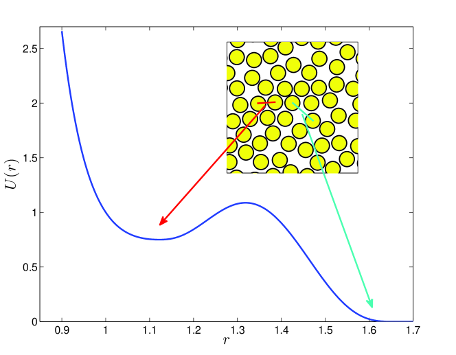
Figure 3: The pair-wise potential for the hump model. In the inset we show a snapshot of the position of the point-particles (the circles represent the radius $\sigma$). Note that the two typical scales $r_{\rm min}$ and $r_{\star}$ appear as the typical distances between particles

.

with the parameters as shown in table 1.

$h_{0}$	0.	75
$r_{\mbox{\tiny hump}}$	1.	32
$r_{\star}$	1.	65
$a_{0}$	1.	0
$a_{1}$	0.	0
$a_{2}$	2.	675405732987203
$a_{3}$	46.	593574934286437
$a_{4}$	-212.	021700143354
$a_{5}$	308.	7495934944721
$a_{6}$	-188.	1854149609638
$a_{7}$	41.	188540942572089

Table 1: Parameters used in the potential of the hump model.

Note that the two typical distances that are defined by this potential, i.e. the distance at the minimum $r_{\rm min}$ and the cutoff scale $r_{\star}$, appear explicitly in the amorphous arrangement of the particles in the supercooled liquid, as shown in the inset in Fig. 3. The model has two crystalline ground states, one at high pressure with a hexagonal lattice and a lattice constant of the order of $r_{\rm min}$. At low pressure the ground state is a more open structure in which the distance $r_{\star}$ appears periodically. At intermediate pressures the system fails to crystallize and forms a glass upon cooling.

The great difference between these two models will become even clearer after we define the up-scaled quasi-species below. On the face of it, the scenario for the glass transition appears similar as exemplified in Fig. 4 in which the intermediate scattering function

$$F_{k}(t;T)\equiv\left\langle\frac{1}{N}\sum_{i=1}^{N}\exp\left\{{i{\bm{k}}\cdot[{\bm{r}}_{i}(t)-{\bm{r}}_{i}(0)]}\right\}\right\rangle\ .$$ (4)

is shown for $k=6.16\sigma^{-1}$. The hump model was simulated using the same algorithms as the binary model, but without the Berendsen barostat that was unneeded for the NVT ensemble.

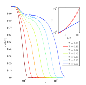
Figure 4: Color online: Time dependence of the correlation function 4 in the hump model for a range of temperatures as shown in the figure. Inset: the temperature dependence of the relaxation time $\tau_{\alpha}(T)$.

.

The relaxation time $\tau_{\alpha}$ for the hump model is shown in Fig. 4 in which we stress again the difference between the region in which there is Arrhenius behavior and the region where the relaxation time grows faster than $\exp(E/T)$.

III Choice of up-scaled variables and validation

Our aim is to provide a theory that captures, when the temperature goes down, the subtle changes in the structural organization of the particles; this rearrangement is in fact directly responsible for the glass transition. The first step in our approach is up-scaling, (or coarse-graining) from particles to quasi-species that can be characterized by their enthalpy and degeneracy. Up-scaling is an art, since it can be done in various ways and there is no unique algorithm to select a-priori a ‘best’ up-scaling. Therefore we need to validate the choice of up-scaled variables using a criterion that was introduced in 09LPZ . The up-scaling is typically different for different models, and we describe it separately for the two models at hand.

III.1 Up-scaling of the binary model

The potential in the case of the binary model is purely repulsive and it has well defined range of interaction $r_{c}(i,j)$ for any given pair of particles. A natural up-scaling for this potential is provided by the particles and their nearest neighbors, where ‘neighbors’ are defined as all the particles $j$ around a chosen central particle $i$ that are within the range of interaction $r_{c}(i,j)$. We refer to the type of a central particle (small or large) in combination with the amount of its nearest neighbors to define the quasi-species. In the interesting range of temperatures we find 8 quasi-species with one ‘small’ central particle and $3,4\dots 10$ neighbors, and 9 quasi-species with one ‘large’ central particle with $6,7\dots 14$ neighbors, all in all 17 quasi-species. Other combinations have negligible concentration ($<0.5\%$) throughout the temperature range. We denote these quasi-species as $C_{s}(n)$ and $C_{\ell}(n)$ with $s$ and $\ell$ denoting the small or large central particle, while $n$ denotes the number of neighbors. We measured the mole-fractions $\langle C_{s}(n)\rangle(T)$ and $\langle C_{\ell}(n)\rangle(T)$ and the results are shown in Fig. 5.

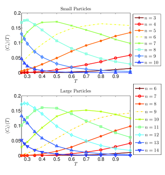
Figure 5: Color online: Temperature dependence of the concentrations of the quasi-species of the binary model. Symbols are simulation data and the lines are a guide to the eye.

We see that some concentrations decrease upon decreasing the temperature, others increase, and yet some first increase and further decrease. We submit to the reader that the subtle changes in configurational arrangement as seen in this plot encode the scenario of the glass transition in a way that we will attempt to decode below.

III.2 Up-scaling of the hump model

The potential of the hump model has a distinct minimum which suggests that quasi-species could consist of each particle and all its neighbors which are within the minimum. This type of up-scaling may have a limited usefulness when the temperature is sufficiently high to allow easy escape over the maximum. The glass transition occurs however in a temperature range where $T$ is lower than the maximum, and we expect the chosen up-scaling to be sensible throughout the interesting temperature range. In this range we find quasi-species with 2, 3, 4, 5 and 6 neighbors within the minimum. In Fig. 6 we show the temperature dependence of the quasi-species of this model which are denoted as $C_{i}$ with $i=2,3,\dots,6$ being the number of neighbors within the minimum.

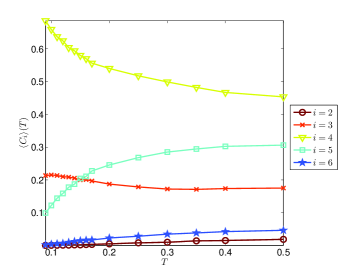
Figure 6: Color online: Temperature dependence of the concentrations of the quasi-species of the hump model. Symbols are simulation data and the lines are a guide to the eye.

The reader should be sensitive to the distinction between the two models. The quasi-species in the binary model can change upon every cage vibration; anytime the distance between two particles exceeds or goes below $r_{c}$ the definition of the quasi-speices changes. On the other hand in the hump model the quasi-species are much more stable, since an exchange of a particle calls for an escape or penetration by going over the hump. We have chosen the models to have these clear differences in order to test the generality of our approach.

III.3 Validation of the up-scaling

Since there is no unique algorithm to choose the up-scaling, we need to have a criterion that validates or rejects the choice of quasi-species. In ref. 09LPZ such a criterion was introduced as explained next.

III.3.1 Validation of the up-scaling in the binary model

To decide whether the up-scaling provides a useful statistical mechanics for the binary model we now ask whether there exist free energies ${\mathcal{F}}_{s}(n;T)$ and ${\mathcal{F}}_{\ell}(n;T)$ such that

$$\langle C_{s}(n)\rangle(T) = \frac{e^{-{\mathcal{F}}_{s}(n;T)/T}}{2\sum_{n=3}^{10}e^{-{\mathcal{F}}_{s}(n;T)/T}}\ ,$$

$$\langle C_{\ell}(n)\rangle(T) = \frac{e^{-{\mathcal{F}}_{\ell}(n;T)/T}}{2\sum_{n=6}^{14}e^{-{\mathcal{F}}_{\ell}(n;T)/T}}\ .$$ (5)

The free energies are found by inverting Eqs. (5) in terms of the measured concentrations. In doing so one can always choose one of the concentration to have by definition zero free energy. This is because the constraint $\sum_{n}C_{s}(n)+\sum_{n}C_{\ell}(n)=1$ makes the system of equations overdetermined. Then the free energies of all the other quasi-species are actually the difference from this chosen reference particle. We then plot these quantities as a function of the temperature, as demonstrated for the present case in Fig. 7.

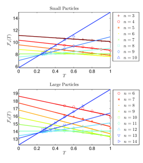
Figure 7: Color online: The approximate linear dependence of the free energies of the chosen quasi-species on the temperature. From the slope we read the degeneracy and from the intercept the enthalpies (up to normalization), cf. Eq. 6. Note that when the free energies are large we do not have data: the concentrations become exponentially small and in a finite simulation box they disappear completely.

We say that our upscaling is validated if ${\mathcal{F}}_{s}(n;T)$ and ${\mathcal{F}}_{\ell}(n;T)$ can be well approximated as linear in the temperature. Then we can interpret

$${\mathcal{F}}_{s}(n;T) \equiv \mathcal{H}_{s}(n)-T\ln g_{s}(n)\ ,$$

$${\mathcal{F}}_{\ell}(n;T) \equiv \mathcal{H}_{\ell}(n)-T\ln g_{\ell}(n)\ ,$$ (6)

where now the degeneracies $g_{s}(n)$ and $g_{\ell}(n)$ (read from the slopes in Fig. 7) and enthalpies ${\mathcal{H}}_{s}(n)$ and ${\mathcal{H}}_{\ell}(n)$ (read from the intercepts) are temperature-independent. This validates the choice of up-scaling. In other words, the approximate linearity of the inverted free energies in the temperature means that we can write the concentrations as

$$\langle C_{s}(n)\rangle(T) \approx \frac{g_{s}(n)e^{-\mathcal{H}_{s}(n)/T}}{2\sum_{n=3}^{10}g_{s}(n)e^{-\mathcal{H}_{s}(n)/T}}\ ,$$

$$\langle C_{\ell}(n)\rangle(T) \approx \frac{g_{\ell}(n)e^{-\mathcal{H}_{\ell}(n)/T}}{2\sum_{n=6}^{14}g_{\ell}(n)e^{-\mathcal{H}_{\ell}(n)/T}}\ .$$ (7)

Then we can use these forms also as a prediction for temperatures where the simulation time is too short to observe the relaxation to equilibrium. The resulting degeneracies $g_{s}(n)$ and $g_{\ell}(n)$ can be easily modeled by a Gaussian distribution around the most probable number $n_{\rm mp}$ of nearest neighbors for small and large particles respectively:

$$g_{s}(n) \approx e^{-[(n-n^{s}_{\rm mp})^{2}/2\sigma^{2}_{s}]}\ ,\quad n^{s}_{\rm mp}=4.65,\sigma^{2}_{s}=1.55\ ,$$

$$g_{\ell}(n) \approx e^{-[(n-n^{\ell}_{\rm mp})^{2}/2\sigma^{2}_{\ell}]}\ ,\quad n^{\ell}_{\rm mp}=7.50,\sigma^{2}_{\ell}=2.0\ .$$ (8)

The analytic fit to the measured degeneracies is shown in Fig. 8, upper panel. The same figure shows in the middle panel the enthalpies of the various quasi-species. One could model the enthalpies as a linear function in $n$. These results are easily interpreted; we have high enthalpies when there are large free volumes (few neighbors). The lowest enthalpies are found when there are many neighbors and there is no much costly free volume. In other words, at the present density and range of temperatures the $pV$ term dominates the energy in the enthalpy. Using the theoretical degeneracies and the measured enthalpies we compute the concentrations of all our quasi-species and compare them with the measurement in the lowest panel of Fig. 8. The agreement that we have, especially considering the number of quasi-species and the simplicity of the theory, is very satisfactory. Notice that the competition between degeneracy and enthalpy explains the rather intricate temperature-dependence of the concentrations of the quasi-species, sometimes declining when the temperature drops, sometime rising, and sometime having non-monotonic behavior.

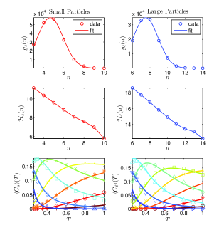
Figure 8: Color online: Upper panel: The degeneracies $g_{s}(n)$ and $g_{\ell}(n)$ read from the slopes of Fig. 7 (in circles) and the degeneracies according to the gaussian model Eq. (8). Middle panel: the measured enthalpies. Lower panel: comparison of the measured concentrations of quasi-species to those calculated from Eqs. (7) using the model degeneracies and measured enthalpies. Here symbols are data and lines are theoretical predictions.

III.3.2 Validation of the up-scaling in the hump model

Validating the up-scaling in the hump model follows the same ideas as in the binary model. We choose the quasi-species $n=2$ as the reference concentration with $F_{2}\equiv 0$ and then invert the data for $\langle C_{i}\rangle(T)$ to find the free energies via

$$\langle C_{i}\rangle(T)=\frac{e^{-\mathcal{F}_{i}(T)/T}}{\sum_{2}^{6}e^{-\mathcal{F}_{i}(T)/T}}\ .$$ (9)

The observed linearity of $\mathcal{F}_{i}(T)$ in the temperature means that we can write

$$\mathcal{F}_{i}(T)=\mathcal{H}_{i}-T\ln g_{i}\ ,$$ (10)

where ${\mathcal{H}}_{i}$ is the enthalpy and $g_{i}$ the degeneracy of the $i$th quasi-specie. The test of linearity from which we can read the energies and degeneracies is shown in Fig. 9.

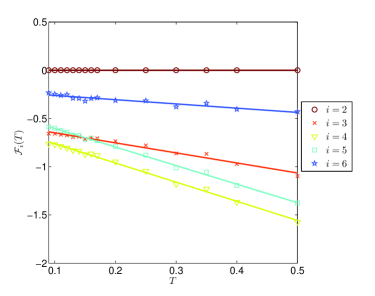
Figure 9: Color online: The approximate linear dependence of the free energies of the chosen quasi-species on the temperature in the hump model. From the slope we read the degeneracy and from the intercept the energies(up to normalization), cf. Eq. 10.

From the intercepts of the lines in Fig. 9 we read the enthalpies, and from the slopes we read the degeneracies. The resulting numerical values are shown in Table 2.

$\mathcal{H}_{2}$	0.	$g_{2}$	1.
$\mathcal{H}_{3}$	-0.545053	$g_{3}$	2.830972
$\mathcal{H}_{4}$	-0.564547	$g_{4}$	7.289318
$\mathcal{H}_{5}$	-0.411079	$g_{5}$	6.862693
$\mathcal{H}_{6}$	-0.217412	$g_{6}$	1.552314

Table 2: Temperature independent enthalpies and degeneracies of the sub-species of the hump model.

Since the hump model is studied in the NVT ensemble the reader may ask why we get enthalpies rather than energies. The reason is that the upscaling using the index $i$ takes into account only the particles that reside inside the hump. The energy of a quasi-species with $i$ particles within the hump is proportional to $i$, and thus for low temperatures the energetically preferred subspecies would be the one with no neighbors within the hump. Clearly this arrangement does not satisfy the constant volume constraint which needs to be taken into account. Indeed, what we call enthalpies cannot be straight energies, otherwise the energies should have been proportional to $i$, making ${\mathcal{H}}_{2}$ the smallest rather than the largest.

III.4 Summary of the statistical mechanics

We can summarize the findings up to now by saying that at least in terms of capturing the scenario of the changes in the spatial organization of the particles our statistical mechanics appears very suitable. Our quasi-species appear to have very well defined enthalpies and degeneracies and we can therefore capture the temperature dependence of the concentrations of the quasi-particles with high accuracy. Our thesis is that this scenario is actually the scenario of the glass transition, and hidden in it is also the reason for the slowing down, as demonstrated in the next section. Intuitively the picture should be clear already now. As the temperature reduces the quasi-species with high free energy tend to disappear, leaving us with quasi-species of low free energy. Then the dynamics become more constrained, since it is more costly to change objects of low free energy (creating on the way objects of higher free energy) than at high temperature when there are many objects with high free energy that can readily change to objects of lower free energy. What we need now is to make this observation more quantitative.

IV Relation to Dynamics

In this section we connect the structural theory to the dynamical slowing-down. To this aim we note that in both models there are a number of quasi-species whose concentration goes down exponentially (or maybe faster) when the temperature decreases, and that the relaxation time shoots up at the same temperature range. We refer to these quasi-species as the ‘liquid’ ones; These are the quasi-species that are prevalent when the temperature is high but are getting rare when the temperature goes down. We discuss now the connection between this phenomenon and the slowing down.

IV.1 The binary model

In this example the ‘liquid’ concentrations are those consisting of small particles with 3-7 neighbors, and large particles with 6-11 neighbors, see Fig. 10 footnote . We sum up these concentrations and denote the sum as $\langle C_{\rm liq}\rangle(T)$. The dependence of $\langle C_{\rm liq}\rangle(T)$ on the temperature is shown in Fig. 10.

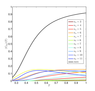
Figure 10: Color online: The temperature dependence of $C_{\rm liq}(T)$ is shown as the upper continuous line. The contributions of the various ‘liquid’ sub-species are shown with symbols which are identified in the inset.

This concentration is used to define a typical scale,

$$\xi(T)\equiv[\rho C_{\rm liq}(T)]^{-1/3}\ ;$$ (11)

where $\rho$ is the number density. This length scale has the physical interpretation of the average distance between the ‘liquid’ quasi-species. It was argued before 07ILLP ; 08LP ; 08EP that this length scale can be also interpreted as the linear size of relaxation events which include $O(\xi(T))$ quasi-species. We can therefore estimate the growing free energy per relaxation event as $\Delta G=\mu\xi(T)$ where $\mu$ is the typical chemical potential per involved quasi-species. This estimate, in turn, determines the relaxation time as

$$\tau_{\alpha}(T)=e^{\mu\xi(T)/T}\ .$$ (12)

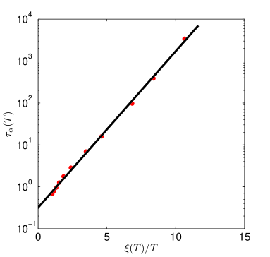
Figure 11: Color online: The relaxation time $\tau_{\alpha}(T)$ in terms of the typical scale $\xi(T)$ in the binary model. We show the excellent fit to Eq. (12) with $\mu=0.37$. Note that the intercept at $T\to\infty$ is of the order of unity as it must be.

The quality of this prediction can be gleaned from Fig. 11, where we can see that the fit is excellent, with $\mu\approx 0.3$. The intercept in Fig. 11 is of the order of unity; this is very reassuring, since this is what we expect when $T\to\infty$.

IV.2 The hump model

In this model the quasi-species whose concentration goes to zero rapidly in the relevant temperature range are those with $i=2,5$ and 6. In Fig. 12 we see their temperature dependence and also their sum which is again denoted as $C_{\rm liq}(T)$. Since in this model we are in two dimensions, the typical scale $\xi(T)$ is related to $C_{\rm liq}(T)$ according to

$$\xi(T)\equiv[\rho C_{\rm liq}(T)]^{-1/2}\ ;$$ (13)

With this obvious change we expect Eq. (12) to be valid also here, and indeed in Fig. 13 we see that this expectation is wonderfully fulfilled.

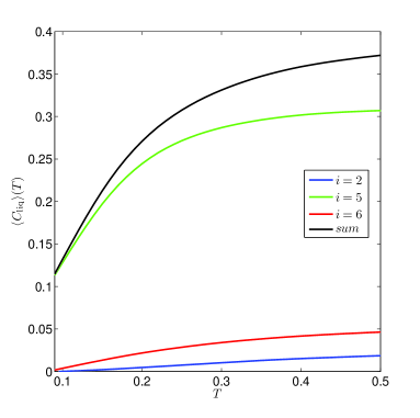
Figure 12: Color online: The quasi-species contributing to $C_{\rm liq}(T)$ in the hump model, and the temperature dependence of the their sum, which is $C_{\rm liq}(T)$.

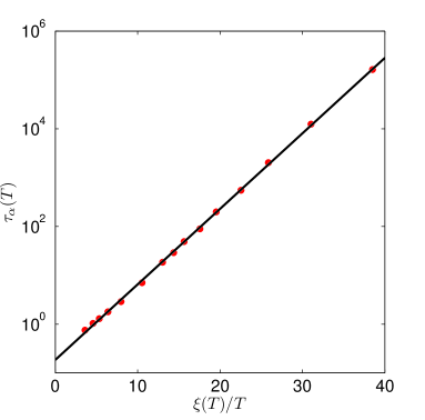
Figure 13: Color online: The relaxation time $\tau_{\alpha}(T)$ in terms of the typical scale $\xi(T)$ in the hump model. We show the excellent fit to Eq. (13) with $\mu=0.34$. Note that the intercept at $T\to\infty$ is of the order of unity as it must be.

IV.3 Pertinent Remarks

A few points should be stressed. As we expect (cf. Ref 08EP ), in systems with point particles and soft potential, there is no reason to fit the relaxation time to a Vogel-Fulcher form 96EAN which predicts a singularity at finite temperature. In our approach we predict that $\xi\to\infty$ only when $T\to 0$, and there is nothing singular on the way, only slower and slower relaxation. At some point the simulation time will be too short for the system to relax to equilibrium, but we can use Eq. (12) to predict what should be the simulation time to allow the system to reach equilibrium. It is important to bear in mind that finite systems of point particles with soft potential are different from finite granular media or systems of hard spheres which can truly jam and lose ergodicity. Point particles with soft potential remain ergodic 08EP , and therefore should be amenable in their super-cooled regime to statistical mechanics. We argue that in order to construct simple, workable statistical mechanics one needs to up-scale the system and find a collection of quasi-species with well defined enthalpies and degeneracies. In this paper we showed that the simple criterion to validate the choice of up-scaling which was suggested in 09LPZ can be applied to very different models once we select the proper up-scaling. Once the structural theory is under control, a natural length scale appears and can be used to determine the relaxation time, also for temperatures that cannot be simulated due to the fast growth of the relaxation time. The fact that the present approach works equally well in two and three dimensions, in NPT and NVT ensembles and in very different models provides good reason to believe that it has a substantial degree of generality.

V The thermodynamics of glass forming systems

As a last issue we raise the following question: is the statistical mechanical theory as defined on the up-scaled quasi-species determining also the thermodynamics of the original system on the particle level. The answer to this question is not obvious a-priori, but turns out to be in the affirmative. As done throughout this paper, we demonstrate this point separately for the two models at hand.

V.1 Thermodynamics of the binary model

The binary model is studied in the NPT ensemble and therefore the first question to ask is whether the average enthalpy of the quasi-species represents the correct enthalpy of the system. In other words, we have extracted the enthalpies $H_{s}(n,T)$ and $H_{\ell}(n,T)$. Is it then true that the enthalpy of the system, computed as the average potential energy summed over all the pairs of particles and summed with $pV$ should equal the enthalpy of the quasi-species:

$$\sum_{n=3}^{10}C_{s}(n){\mathcal{H}}_{s}(n,T ) +\sum_{n=6}^{14}C_{\ell}(n){\mathcal{H}}_{\ell}(n,T)$$ (14)

$$= \frac{1}{2N}\sum_{i,j=1}^{N}\langle U(r_{ij})\rangle+pV(T)\ .$$

In answering this question we remember that our enthalpies are defined up to an arbitrary constant since we chose one of the quasi-species as a reference with zero free energy. We can therefore add or subtract an arbitrary constant from the LHS or the RHS of Eq. 14. In Fig. 14 we show the ratio of the LHS of Eq. (14) to the RHS, with the conclusion that the enthalpy of the system is excellently reproduced by the up-scaled variables.

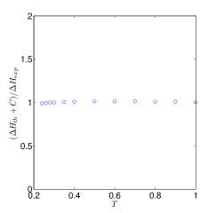
Figure 14: Color online: The ratio of the LHS of Eq. (14), denoted as $\Delta H_{\rm th}+C$ (here, $C=2.8$) over the RHS of Eq. (14), denoted $\Delta H_{\rm exp}$. We conclude that the enthalpy of the system is excellently reproduced by the up-scaled variables.

Needless to say, we could therefore compute the specific heat at constant pressure, $C_{p}$, from either set of data, and from that we could get the entropy of the system, reassuring us that the up-scaling method, once validated as above, provides also the correct thermodynamics for the glass forming system. In the next subsection we show actual computations of such thermodynamic quantities.

V.2 Thermodynamics of the hump model

The hump model was studied in the NVT ensemble, and therefore it is interesting to test whether one obtains the correct system’s energy. The potential energies of the quasi-species which were characterized by the number of neighbors that are bound within the minimum are to an excellent approximation linear in that number, $E_{i}=0.83i$ as measured with respect to the same zero point as that of the potential (3). We therefore need to check whether

$$\frac{0.83}{2}\sum_{i=2}^{6}C_{i}(T)i+T=\frac{1}{2N}\sum_{i,j=1}^{N}\langle U(r_{ij})\rangle\ .$$ (15)

We have added $T$ for the excitation around the ground state of the quasi-species (two degrees of freedom in 2D). This test is shown in Fig. 15 where the predictions of the theory were extrapolated all the way

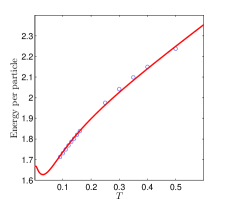
Figure 15: Color online: Comparison of the LHS of Eq. (15) in red continuous line, to the RHS of the same equation, in symbols. We conclude that the energy of the system is excellently reproduced by the up-scaled variables down to temperatures of about $T\approx 0.05$ For lower temperatures the extrapolation obviously fails.

to zero temperature. Obviously the data loses its predictability somewhere around $T=0.05$ where the specific heat becomes negative. This artifact is seen even better in the plot of the specific heat which is offered in Fig. 16.

Figure 16: Color online: Symbols: the derivative with respect to $T$ of the RHS in Eq. (15). Continuous line: derivative with respect to $T$ of the LHS in Eq. (15). The theory predicts the expected specific heat peak and fails when the specific heat becomes negative.

Nevertheless the plot of $C_{v}$ vs. $T$ indicates the expected typical specific heat peak around $T=0.1$ which could not be seen in the simulations due to the inherent limitations of computer time. Once the specific heat takes a dive, at some point we can no longer believe the extrapolation, and more accurate data are necessary to be able to predict the thermodynamic properties near zero temperatures.

VI Summary and the road ahead

In summary, we have shown how the scenario of the glass transition can be neatly characterized by the temperature dependence of the concentrations of the various quasi-species that are obtained after up-scaling. Those quasi-species that are readily changed because they are rich in free energy are of course those that deplete first. We are left with quasi-species that are low in free energy, and these would naturally be hard to change since their change necessarily increases the free energy. The presumed ergodicity allows us to introduce statistical mechanics which can beautifully encode the scenario, using a small number of quasi-species together with their enthalpies and degeneracies. The statistical mechanics applies also at temperatures that are beyond the range available to molecular simulations, and can be used to predict what is happening there. We have shown that when the upscaling and the statistical mechanics work well, the thermodynamics of the system can be understood very well using the up-scaled picture.

There are still issues to understand. One of our main concerns is how to achieve a first-principles prediction of the parameter $\mu$ in Eq. (12). We have, so far, been unable to bridge this gap, leaving the connection between the dynamics and the upscaling theory still dependent on a phenomenological fit. A satisfactory prediction of $\mu$ would, in our opinion, close the loop and put to rest the riddle of the slowing down in the glass-forming systems. Also, the upscaling approach had been so far limited to computer model of glass formation, we propose that it would be enlightening to try and apply it to real experimental systems. We hope that these and other issues would be clarified in future research.

- (1) For a general review cf. M. D. Ediger, C. A. Angell, and S. R. Nagel, J. Phys. Chem. 100, 13200 (1996).
- (2) J-P. Eckmann and I. Procaccia, Phys. Rev. E, 78, 011503 (2008).
- (3) E. Aharonov, E. Bouchbinder, V. Ilyin, N. Makedonska, I. Procaccia and N. Schupper, Europhys. Lett. 77, 56002 (2007) .
- (4) H. G. E. Hentschel, V. Ilyin, N. Makedonska, I. Procaccia and N. Schupper, Phys. Rev. E 75, 050404 (2007).
- (5) V. Ilyin, E. Lerner, T-S. Lo and I. Procaccia, Phys. Rev. Lett., 99, 135702 (2007).
- (6) E. Lerner and I. Procaccia, Phys. Rev. E 78, 020501 (2008).
- (7) E. Lerner, I. Procaccia and I. Regev, Phys. Rev E, in press. Also: arXiv:0806.3685.
- (8) E. Lerner, I. Procaccia, and J. Zylberg Phys. Rev. Lett. 102, 125701 (2009).
- (9) H. G. E. Hentschel, V. Ilyin and I. Procaccia, Phys. Rev. Lett. 101 265701 (2008)
- (10) H. G. E. Hentschel, V. Ilyin, I. Procaccia and N. Schupper, Phys. Rev. E, 78 061504 (2008).
- (11) M.P. Allen and D.J. Tildesley, Computer Simultions of Liquids (Oxford University Press, 1991).
- (12) W. Kob and H. C. Andersen, Phys. Rev. E 51, 4626 (1993).
- (13) D. Deng, A. Argon. and S. Yip, Philos. Trans. R. Soc. London, Ser. A 329 549 (1989).
- (14) D. N. Perera and P. Harrowell, Phys. Rev. E 59, 5721 (1999).
- (15) N. P. Bailey, U. R. Pedersen, N. Gnan, T. B. Schrder, and J. C. Dyre, J. Chem. Phys. 129, 184507 (2008).
- (16) M. Dzugutov, Phys. Rev. A 40, 5434 (1989).
- (17) See for exemple: A.C. Pan, J.P. Garrahan and D. Chandler, Phys. Rev. E 72, 041106 (2005).
- (18) Note that in 09LPZ a smaller set of quasi-species was identified with . In the present treatment we include in this set all the quasi-species whose concentration goes down significantly in the relevant range of tempeartures, and as a result we find a much improved relation between the compositional and dynamical aspects as seen in Fig. 11.