Fermi liquid theory for SU(N) Kondo model

Abstract

We extend the Fermi liquid theory of Nozières by introducing the next-to-leading order corrections to the Fermi liquid fixed point. For a general SU(N) Kondo impurity away from half-filling, this extension is necessary to compute observables (resistivity, current or noise) at low energy. Three additional contributions are identified and their coupling constants are related using an original (and more complete) formulation of the Kondo resonance floating. In the conformal field theory language, a single cubic operator is proposed that produces the same three contributions with the same coupling constants. Comparison with an exact free energy expansion further relates the leading and next-to-leading order corrections so that a single energy scale, the Kondo temperature, eventually governs the low energy regime. We compare our results at large $N$ with the approach of Read and Newns and find analytical agreement.

I Introduction

The fascination exerted by the Kondo model hewson1993 is probably due to the large variety of theoretical techniques invented to describe it. In fact, it has proven quite difficult to find a single approach that alone explains all features of the Kondo model. This is particularly true in out-of-equilibrium situations oguri2001+meir2002+rosch2003+kehrein2005+mehta2006+anders2008 , for example when a bias voltage is applied to a source-drain setup. The seminal papers of Nozières nozieres1974a ; nozieres1974b+nozieres1978 on the Fermi liquid (FL) theory have provided a remarkable insight into the low energy regime of the Kondo model. Based on a phenomenological picture, this approach contains nevertheless all relevant physics and leads to predictions that are exact, albeit perturbative. The most famous example is certainly the Wilson ratio, predicted by Nozières nozieres1974a to be exactly two in agreement with numerical estimates by Wilson wilson1975 . Finally, the FL picture provides a straightforward tool to study analytically the out-of-equilibrium regimes.

The FL approach has been recast later in the more formal language of conformal field theory (CFT) by Affleck and Ludwig affleck1990 ; affleck1991 ; affleck1993 . In this framework, the quasiparticles of the FL constitute a boundary free field theory affleck1990 which is the infrared strong coupling fixed point of the Kondo model. The low temperature regime is then dominated by the leading irrelevant operator at this fixed point and the results affleck1993 are in complete agreement with Nozières. More recently, elaborating on a more involved version of the Bethe ansatz, Lesage and Saleur lesage1999a+lesage1999b were able to justify the FL theory for ordinary SU(2) Kondo and to extend it to all leading irrelevant operators. To be more exhaustive, we shall mention the work of Yosida and Yamada published independently from Nozières. In a series of papers yosida1970+yamada1975a+yosida1975+yamada1975b on the parent Anderson model, they did a thorough analysis of perturbation theory in the interaction term $U$. They derived general low energy properties for the self-energy that proved the Fermi liquid picture extending it to finite $U$. The extension of their work to the second order low energy corrections is yet an unsolved problem. Aside from these works and perhaps surprisingly, the FL theory as presented by Nozières was not pursued much further hewson1993 ; hewson1994 , probably because no simple means were known to relate the different phenomenological coefficients of the theory. Following studies have started instead to focus on more exotic non-Fermi liquid regimes affleck1991 ; affleck1993 ; nozieres1980 .

Originally discussed for an ordinary spin-$1/2$ impurity with SU(2) symmetry, the FL fixed point constitutes more generally the low energy limit of the Kondo model for a SU(N) hyperspin impurity. The value of $N$ tunes the relative importance of the different low energy processes. This SU(N) Kondo model is called the Coqblin-Schrieffer model coqblin1969 for a single-electron impurity. Both this model and its parent Anderson model have exact Bethe ansatz solutions andrei1983+tsvelik1982+rasul1982 ; schlottmann1982+tsvelik1983 . The SU(4) case has a particular experimental relevance with recent achievements in vertical quantum dots sasaki2004 and carbon nanotubes herrero2005+makarovski2007a+makarovski2007b ; delattre2009 . In those experiments, an orbital degeneracy might combine with the usual spin-$1/2$ to form an intricate SU(4) symmetry.

The conventional Fermi liquid description contains only the leading irrelevant operators of dimension $3$, also linear in $1/T_{K}$ where $T_{K}$ is the Kondo temperature. These operators include a combination of an elastic channel with an inelastic one. The ratio of elastic to inelastic scattering amplitudes is fixed by the Friedel sum rule langreth1966 or more generally by the principle of floating of the Kondo resonance that we shall detail in the core of this article. This fixed ratio can also be shown to be a consequence of the vanishing charge susceptibility on the dot hewson1994 . The conventional FL approach, as we described, is sufficient to compute observables that have a linear energy ($k_{B}T$, $eV$ or $\mu_{B}B$) dependence, hence the success in the determination of Wilson’s ratio even for a general SU(N) symmetry nozieres1980 . However, for observables with a quadratic behavior such as the resistivity or the conductance, the addition of dimension-$4$ operators becomes necessary. The ordinary SU(2) Kondo effect is peculiar in this respect since the coefficients of these new dimension-$4$ operators identically vanish.

The purpose of this paper is to extend the conventional FL approach by introducing the full set of dimension-$4$ operators with their coefficients. Within the theoretical framework proposed by Nozières, this second generation adds three terms to the conduction electron phase shift. One represents elastic scattering and two inelastic scattering involving the excitation of one and two electron-hole pairs. The ratios between the coefficients of the three FL corrections are then fixed by using the floating of the Kondo resonance. Let us emphasize that the picture built in this article for the Kondo resonance floating extends the initial vision of Nozières. Not only the peak of the resonance is tied to the Fermi singularity but also the whole structure of the resonance. We also investigate how this translates into the CFT language. A single dimension-$4$ operator is identified with SU(N) invariance. Its expansion on the electron fields recovers the aforementioned three processes with the same coefficient ratios. Last step of the analysis, the free energy as a function of generalized magnetic fields can be easily calculated within the FL theory including all dimension-$3$ and dimension-$4$ operator sets. Comparing the result with the exact solution obtained from an alternative Bethe ansatz bazhanov2003 , the ratio between dimension-$3$ and dimension-$4$ corrections can be determined. All coefficients are finally related to each other so that, as expected, universality is recovered as $T_{K}$ remains the only energy scale in the problem. This completes our full characterization of the low energy FL theory for the Kondo SU(N) model. We stress again that this work does not modify (and therefore does not contradict) the ordinary SU(2) analysis glazman2005 since the new FL corrections are vanishing in that case. However these new corrections are fundamental in the more general SU(N) case where particle-hole symmetry is broken.

The idea of introducing the next-to-leading order FL corrections was first formulated in Ref. vitu2008 , although incompletely. It was however not taken into account in Ref. lehur2007 . The current and the noise through a SU(N) Kondo quantum dot were calculated in Refs. vitu2008 ; mora2008 , with a correction in mora2009 on the basis of this work. The rest of this article is organized as follows: the new FL corrections are introduced in the usual FL framework in Sec. II with an emphasis on the Kondo floating; and in the CFT language in Sec. III. Sec. IV compares the free energy with the exact Bethe ansatz solution. Sec. V proceeds with a $1/N$ expansion which coincides with the field theoretical large $N$ approach of Read and Newns newns1987 . Sec. VI concludes.

II Fermi liquid theory

Let us define the problem more precisely. The starting Kondo Hamiltonian is (we follow Einstein convention for the capital superscripts)

$$H=\sum_{k,\sigma=1\ldots N}\varepsilon_{k}b_{k\sigma}^{\dagger}b_{k\sigma}+J_{K}S^{A}\,\sum_{k,k^{\prime},\sigma,\sigma^{\prime}}b_{k\sigma}^{\dagger}T^{A}_{\sigma,\sigma^{\prime}}b_{k^{\prime}\sigma^{\prime}},$$ (1)

with the dispersion $\varepsilon_{k}=\varepsilon_{F}+\hbar v_{F}k$ linearized around the Fermi energy $\varepsilon_{F}$. $b_{k\sigma}$ is the annihilation operator for a conduction electron with spin $\sigma$ and wavevector $k$ (measured from $k_{F}$). The Kondo interaction, controlled by $J_{K}$, is an antiferromagnetic coupling between the impurity spin operator $\vec{S}=\{S^{A}\}$ and the spin operator of the conduction electrons at $x=0$ (impurity site). $T^{A}$ and $S^{A}$ are two sets of $N^{2}-1$ generators satisfying the commutation relations

$$\vspace*{1.cm}[S^{A},S^{B}]=if_{ABC}S^{C},\quad[T^{A},T^{B}]=if_{ABC}T^{C},$$ (2)

where the antisymmetric tensors $f_{ABC}$ are the structure factors of the SU(N) Lie algebra. The matrices $T^{A}$ generate the fundamental representation of $SU(N)$ while the $S^{A}$ define the antisymmetric representation of $SU(N)$ corresponding to a Young tableau of a single column with $m$ boxes. Physically, the Kondo Hamiltonian (1) emerges from an Anderson model with exactly $m$ electrons at the impurity site.

In the ground state of the model, the spin of the impurity forms a singlet with conduction electrons. It is therefore completely screened and disappears from the picture at low energy. The Fermi liquid theory describes the low energy regime and is built on the following assumptions: (i) the singlet scatters elastically conduction electrons, (ii) virtual polarization of the singlet leads to weak interactions between conduction electrons of different spin and, (iii) the energy of the system is an analytical function only of the bare energies $\varepsilon_{k}$ and of the relative quasiparticle occupation numbers $\delta n_{\sigma}(\varepsilon)$. More precisely, $\delta n_{\sigma}(\varepsilon)=n_{\sigma}(\varepsilon)-\theta(\varepsilon_{F}-\varepsilon)$ is the actual occupation number relative to the ground state distribution with Fermi energy $\varepsilon_{F}$. The last point (iii) is in fact the most stringent one and it is reminiscent of the usual (bulk) Fermi liquid theory. Instead of considering the total energy, one can concentrate on the energy shift of a single quasiparticle excitation and, by imposing boundary condition for a system of finite size, translate it into an electron phase shift at energy $\varepsilon$. $\delta_{\sigma}(\varepsilon,\delta n_{\sigma^{\prime}})$ is therefore an analytical function that depends only on $\varepsilon$ and on the functions $\delta n_{\sigma^{\prime}}(\varepsilon)$.

The general expansion of the phase shift (hereafter $\sum_{\varepsilon}$ stands for $\int d\varepsilon$)

$$\begin{split}\delta_{\sigma}(\varepsilon,\delta n_{\sigma^{\prime}})=\delta_{0}&+\frac{\alpha_{1}}{T_{K}}(\varepsilon-\varepsilon_{F})+\frac{\alpha_{2}}{T_{K}^{2}}(\varepsilon-\varepsilon_{F})^{2}-\sum_{\sigma^{\prime}\neq\sigma}\Bigg{(}\frac{\phi_{1}}{T_{K}}\sum_{\varepsilon^{\prime}}\delta n_{\sigma^{\prime}}(\varepsilon^{\prime})\\[2.84526pt] &+\frac{\phi_{2}}{2T_{K}^{2}}\sum_{\varepsilon^{\prime}}(\varepsilon+\varepsilon^{\prime}-2\varepsilon_{F})\,\delta n_{\sigma^{\prime}}(\varepsilon^{\prime})-\frac{\chi_{2}}{T_{K}^{2}}\sum_{\sigma^{\prime\prime}<\sigma^{\prime}\atop\sigma^{\prime\prime}\neq\sigma}\sum_{\varepsilon^{\prime},\varepsilon^{\prime\prime}}\delta n_{\sigma^{\prime}}(\varepsilon^{\prime})\delta n_{\sigma^{\prime\prime}}(\varepsilon^{\prime\prime})\Bigg{)}+{\cal O}\left(\frac{1}{T_{K}^{3}}\right),\end{split}$$ (3)

introduces the dimensionless phenomenological coefficients $\alpha_{1}$, $\alpha_{2}$, $\phi_{1}$, $\phi_{2}$ and $\chi_{2}$. $\delta_{0}$ is the phase shift at the Fermi level. Its value is imposed by the Friedel sum rule,

$$\delta_{0}=\frac{m\,\pi}{N},$$ (4)

so that $\delta_{0}=\pi/2$ at half-filling, i.e. for a particle-hole symmetric situation. Only $\alpha_{1}$ and $\phi_{1}$ are kept in the conventional FL approach nozieres1974a ; glazman2005 . $\alpha_{1,2}$ correspond to elastic scattering. $\phi_{2}$ is an energy correction to the four-point vertex controlled by $\phi_{1}$. $\chi_{2}$ tunes the six-point vertex corresponding to the local interaction of three electrons. The properties of the Kondo resonance can be read from the phase shift expression (3). The phase shift expansion for a resonant level model (RLM) of width $\sim T_{K}$ is similar to the first three (elastic) terms, which identifies $T_{K}$ as the size of the Kondo resonance. The comparison with RLM also indicates that $\alpha_{2}$ is expected to vanish when the resonance is centered at the Fermi level rajan1983 . The dependence of the phase shift (3) on the conduction electron populations is also physically sensible. The Kondo screening is a many-body effect that results from the sharpness of the Fermi surface kondo1964 . The resonance is therefore extremely sensitive to changes in the occupation numbers which modify the shape of the Fermi surface.

The floating of the Kondo resonance follows from the same physical idea. Since the Kondo resonance is built by the conduction electrons themselves, its structure should be invariant when doping the system such that the shapes of electronic distributions remain the same, apart from a global energy shift $\delta\varepsilon$. The only effect of this doping is then to shift the Kondo resonance by $\delta\varepsilon$. Let us implement this physical idea in a practical way. The doping procedure is shown in Fig. 1.

Figure 1: Schematic view of the doping of conduction electrons. The black filled area represents the initial distribution $\delta n(\varepsilon)$ and the grey one the added electrons $\delta n^{1}_{\sigma}(\varepsilon)$. Both the initial and final ($\delta n^{\prime}_{\sigma}(\varepsilon)$) distributions start at $\varepsilon=\varepsilon_{F}$ since the ground state distribution has been subtracted.

$\delta n^{\prime}_{\sigma}(\varepsilon)$ denotes the new distribution and $\delta n^{1}_{\sigma}(\varepsilon)$ the added one such that

$$\delta n^{\prime}_{\sigma}(\varepsilon)=\delta n_{\sigma}(\varepsilon)+\delta n^{1}_{\sigma}(\varepsilon).$$

This translates into $\delta n^{\prime}_{\sigma}(\varepsilon)=\delta n_{\sigma}(\varepsilon-\delta\varepsilon)+\theta(\varepsilon)-\theta(\varepsilon-\delta\varepsilon)$ since $\delta n^{\prime}_{\sigma}$ and $\delta n_{\sigma}$ have the same shape at the right of the energy distribution. The invariance of the Kondo resonance under this doping implies that

$$\delta_{\sigma}(\varepsilon+\delta\varepsilon,\delta n^{\prime}_{\sigma})=\delta_{\sigma}(\varepsilon,\delta n_{\sigma}),$$ (5)

for any $\varepsilon$ and $\delta n_{\sigma}$. Using Eq. (3), it leads to four equations

$$\alpha_{1}-(N-1)\phi_{1} =0,$$ (6a)

$$\alpha_{2}-\frac{3(N-1)}{4}\phi_{2}+\frac{(N-1)(N-2)}{2}\chi_{2} =0,$$ (6b)

$$(N-2)\chi_{2}-\phi_{2}=0,\qquad 2\alpha_{2}-\frac{N-1}{2}\phi_{2} =0,$$ (6c)

corresponding to vanishing coefficients in front of, respectively $\delta\varepsilon$, $\varepsilon\delta\varepsilon$, $\delta\varepsilon\,\sum_{\sigma^{\prime}\neq\sigma,\varepsilon^{\prime}}\delta n_{\sigma^{\prime}}(\varepsilon^{\prime})$ and $(\delta\varepsilon)^{2}$. Eqs. (6) are satisfied with

$$\alpha_{1} =(N-1)\phi_{1},$$ (7a)

$$\alpha_{2}=\frac{N-1}{4}\,\phi_{2}, \qquad\phi_{2}=(N-2)\,\chi_{2}.$$ (7b)

The ratio between $\alpha_{1}$ and $\phi_{1}$ was first obtained in Ref. nozieres1980 . The identities (7) are consistent with the Friedel sum rule but they cannot be simply reduced to it. It is the whole Kondo resonance structure that remains invariant through the energy shift and not only the phase shift at the Fermi energy. To our knowledge, this generalization of the original Nozières’ argument had not yet been pointed out. Note that the Fermi energy $\varepsilon_{F}$ is the only energy reference in this problem, compared to which the system is doped. An alternative and straightforward way to derive Eqs. (6) et (7) is therefore to require the invariance of the phase shift (3) when shifting $\varepsilon_{F}$.

III Conformal field theory

The CFT offers an alternative and illuminating perspective to reexamine these new FL corrections. It was originally noted by Affleck affleck1990 that the fixed ratio between elastic and inelastic terms in the leading FL corrections was a consequence of spin-charge decoupling (spin-charge separation was first shown in Ref. schotte1970 , it also appears in the Bethe ansatz solutions for the Kondo andrei1983+tsvelik1982+rasul1982 and the Anderson schlottmann1982+tsvelik1983 models). Written in terms of (spin) currents, the only eligible dimension-$3$ operator is the square of the spin current operator. This single operator was shown affleck1993 , using standard point-splitting techniques, to produce the two couplings in Nozières’ FL theory, thereby enforcing automatically the relation (7a). We shall see here that the same reduction applies to the second generation of FL terms. One single dimension-$4$ operator can be identified, which produces the couplings $\alpha_{2}$, $\phi_{2}$ and $\chi_{2}$ together with the relations (7b).

The quadratic Hamiltonian describing the strong coupling fixed point

$$H_{0}=\sum_{k,\sigma=1\ldots N}\varepsilon_{k}\psi_{k\sigma}^{\dagger}\psi_{k\sigma},$$ (8)

is written in terms of the quasiparticle field $\psi_{\sigma}(x)=\sum_{k}\psi_{k\sigma}e^{ikx}$. It corresponds to free fermions and the zero-energy phase shift (4) is included in the wavefunction associated to $\psi_{k\sigma}$. The zero-temperature Green’s function is given by

$$\langle\psi^{\dagger}(x)\psi(x^{\prime})\rangle=\frac{i}{2\pi}\frac{1}{x-x^{\prime}}.$$ (9)

The spin current operator $J^{A}(x)=\sum_{\sigma,\sigma^{\prime}}\psi^{\dagger}_{\sigma}(x)T^{A}_{\sigma,\sigma^{\prime}}\psi_{\sigma^{\prime}}(x)$ is written on the basis of SU(N) generators $T^{A}$. The $N\times N$ Hermitian and traceless matrices $T^{A}$ follow Gell-Mann convention azcarraga1998 . The symmetry tensors $d_{ABC}$ bensimon2006 are defined by the multiplication rules

$$T^{A}T^{B}=\frac{1}{2N}\delta_{A,B}\mathds{1}+\frac{1}{2}(d_{ABC}+if_{ABC})T^{C},$$ (10)

compatible with Eq. (2) and where $\mathds{1}$ denotes the unit matrix. The dimension-$3$ FL correction is given by $H_{\rm I}^{(1)}=-\lambda_{1}J^{A}(0)J^{A}(0)$. For the dimension-$4$ operator, we seek a SU(N) invariant form involving three spin currents. The most natural one is

$$H_{\rm I}^{(2)}=-\lambda_{2}\int dx\,\delta(x)\,d_{ABC}:J^{A}(x)J^{B}(x)J^{C}(x):,$$ (11)

which can be seen as a generalization of the cubic Casimir operator of the SU(N) Lie algebra klein1963 . The notation $:\ldots:$ indicates normal ordering of the operators. The invariance over SU(N) rotations can be shown directly using the identity

$$d_{EBC}\,f_{EDA}+d_{AEC}\,f_{EDB}+d_{ABE}\,f_{EDC}=0.$$

The calculation that follows is similar to the one that has been performed for the dimension-$3$ operator in Refs. affleck1993 ; lehur2007 . The product $d_{ABC}J^{A}J^{B}J^{C}$ is obtained from the contraction of the tensor $d_{ABC}T_{ab}^{A}T^{B}_{cd}T^{C}_{ef}$ with six fermionic fields (here $a,b,c,d,e,f$ denote spins). We resort to the identity

$$\begin{split}&d_{ABC}T_{ab}^{A}T^{B}_{cd}T^{C}_{ef}={\cal N}\bigg{(}\frac{N}{2}(\delta_{ad}\delta_{be}\delta_{cf}+\delta_{af}\delta_{bc}\delta_{de})\\[2.84526pt] &+\frac{2}{N}\delta_{ab}\delta_{cd}\delta_{ef}-(\delta_{ab}\delta_{cf}\delta_{de}+\delta_{ad}\delta_{bc}\delta_{ef}+\delta_{af}\delta_{be}\delta_{cd})\bigg{)},\end{split}$$ (12)

with the normalization factor ${\cal N}=(N^{2}-1)/(2N(N^{2}+1))$, in order to avoid the explicit values of the generators $T^{A}$. The singular operator $J^{A}J^{B}J^{C}$ is defined using the standard point-splitting procedure and the normal ordering eventually ensures a regular result.

Using the identity (12) and the explicit point-splitting calculation -with the short distance behavior (9)-, we rewrite the perturbation $H_{\rm I}^{(2)}$ (11) in terms of fermion fields. This is a tedious but straightforward procedure. The result is proportional to the combination

$$\begin{split}&H_{\rm I}^{(2)}\propto-\frac{2}{3}:\psi^{\dagger}_{\sigma}\psi_{\sigma}\psi^{\dagger}_{\sigma^{\prime}}\psi_{\sigma^{\prime}}\psi^{\dagger}_{\sigma^{\prime\prime}}\psi_{\sigma^{\prime\prime}}:\\[2.84526pt] &+(N-2)\frac{i}{2\pi}(\partial_{1}-\partial_{2}):\psi^{\dagger}_{\sigma,1}\psi_{\sigma,2}\psi^{\dagger}_{\sigma^{\prime}}\psi_{\sigma^{\prime}}:\\[2.84526pt] &-\frac{(N-2)(N-1)}{4}\left(\frac{i}{2\pi}\right)^{2}(\partial_{1}-\partial_{2})^{2}:\psi^{\dagger}_{\sigma,1}\psi_{\sigma,2}:,\end{split}$$ (13)

where all fields are taken at $x=0$. For the complete result, we prefer to go to wavevector space. Using that $k=2\pi\nu_{1}\varepsilon_{k}$, where $\nu_{1}=1/(hv_{F})$ is the density of state for chiral 1D fermions, it reads

$$\begin{split}&H_{\rm I}^{(2)}=-\frac{\alpha_{2}}{4\pi\nu_{1}T_{K}^{2}}\sum_{\sigma,\{k_{i}\}}(\varepsilon_{k_{1}}+\varepsilon_{k_{2}})^{2}:\psi_{\sigma,k_{1}}^{\dagger}\psi_{\sigma,k_{2}}:\\[5.69054pt] &+\frac{\phi_{2}}{\pi\nu_{1}^{2}T_{K}^{2}}\sum_{\sigma<\sigma^{\prime},\{k_{i}\}}\frac{\sum_{i=1}^{4}\varepsilon_{k_{i}}}{4}:\psi_{\sigma,k_{1}}^{\dagger}\psi_{\sigma,k_{2}}\psi_{\sigma^{\prime},k_{3}}^{\dagger}\psi_{\sigma^{\prime},k_{4}}:\\[5.69054pt] &-\frac{\chi_{2}}{\pi\nu_{1}^{3}T_{K}^{2}}\sum_{\sigma<\sigma^{\prime}<\sigma^{\prime\prime}\atop\{k_{i}\}}:\psi_{\sigma,k_{1}}^{\dagger}\psi_{\sigma,k_{2}}\psi_{\sigma^{\prime},k_{3}}^{\dagger}\psi_{\sigma^{\prime},k_{4}}\psi_{\sigma^{\prime\prime},k_{5}}^{\dagger}\psi_{\sigma^{\prime\prime},k_{6}}:.\end{split}$$ (14)

Together with the dimension-$3$ operators, Eq. (14) reproduces exactly the phase shift (3). The coefficients $\alpha_{2}$, $\phi_{2}$ and $\chi_{2}$ are related to $\lambda_{2}$,

$$\frac{\alpha_{2}}{\pi\nu_{1}T_{K}^{2}} =3\nu_{1}^{2}{\cal N}\frac{(N^{2}-4)(N^{2}-1)}{2N}\,\lambda_{2},$$ (15a)

$$\frac{\phi_{2}}{\pi\nu_{1}^{2}T_{K}^{2}} =6\nu_{1}{\cal N}\frac{(N^{2}-4)(N+1)}{N}\,\lambda_{2},$$ (15b)

$$\frac{\chi_{2}}{\pi\nu_{1}^{3}T_{K}^{2}} =6{\cal N}\frac{(N+2)(N+1)}{N}\,\lambda_{2},$$ (15c)

so that again we find the Eqs. (7b).

To conclude, we have found independently that the CFT leads to the same three corrections with the same relations (7b) as the FL theory.

IV Input from the Bethe ansatz

In the last two sections, we have shown that we can relate the amplitudes of the different physical processes that appear at a given order in the Hamiltonian perturbative expansion. This can be done either in the FL or in the CFT framework. The arguments that we have used are only based on symmetries and on the global structure of the low energy resonance. What we cannot do however with these phenomenological approaches is to relate the coefficients of the different orders, for instance $\alpha_{1}$ to $\alpha_{2}$ or similarly $\lambda_{1}$ to $\lambda_{2}$. For this, we have to resort to the exact solution of the model, in principle given by the Bethe ansatz solution. Using an alternative Bethe ansatz technique, Bazhanov, Lukyanov and Tsvelik bazhanov2003 have derived analytical expressions for the free energy in the general SU(N) Kondo model with $m$ electrons forming the impurity. We can compute the free energy perturbatively with our model and then compare with the exact solution as a way to extract the relationship between $\alpha_{1}$ and $\alpha_{2}$.

We study the same situation as in Ref. bazhanov2003 . The system is at zero temperature and independent generalized magnetic fields $h_{\sigma}$ are applied to the different spin components. Their chemical potentials are then shifted to $\epsilon_{F}+h_{\sigma}$ (or $h_{\sigma}$ alone if we take $\epsilon_{F}=0$). Since the position of $\epsilon_{F}$ is arbitrary as we have demonstrated in Sec. II, it is chosen such that $\sum_{\sigma}h_{\sigma}=0$. In the FL theory, the free energy is straightforward to calculate from the phase shift (3),

$$\begin{split}F&=F_{0}-\frac{1}{\pi T_{K}}\sum_{\sigma,\varepsilon}\left(\alpha_{1}\varepsilon+\frac{\alpha_{2}}{T_{K}}\varepsilon^{2}\right)\delta n_{\sigma}(\varepsilon)\\[2.84526pt] &+\frac{1}{\pi T_{K}}\sum_{\sigma<\sigma^{\prime}\atop\varepsilon,\varepsilon^{\prime}}\left(\phi_{1}+\frac{\phi_{2}}{T_{K}}\frac{\varepsilon+\varepsilon^{\prime}}{2}\right)\delta n_{\sigma}(\varepsilon)\delta n_{\sigma^{\prime}}(\varepsilon^{\prime})\\[2.84526pt] &-\frac{\chi_{2}}{\pi T_{K}^{2}}\sum_{\sigma<\sigma^{\prime}<\sigma^{\prime\prime}\atop\varepsilon,\varepsilon^{\prime},\varepsilon^{\prime\prime}}\delta n_{\sigma}(\varepsilon)\delta n_{\sigma^{\prime}}(\varepsilon^{\prime})\delta n_{\sigma^{\prime\prime}}(\varepsilon^{\prime\prime}),\end{split}$$ (16)

where $F_{0}$ is the ground state energy. The same expression can be recovered from the Hamiltonian form, with glazman2005 ; sela2006+golub2006+gogolin2006b

$$\begin{split}&H_{\rm I}^{(1)}=-\frac{\alpha_{1}}{2\pi\nu_{1}T_{K}}\sum_{\sigma,\{k_{i}\}}(\varepsilon_{k_{1}}+\varepsilon_{k_{2}}):\psi_{\sigma,k_{1}}^{\dagger}\psi_{\sigma,k_{2}}:\\[5.69054pt] &+\frac{\phi_{1}}{\pi\nu_{1}^{2}T_{K}}\sum_{\sigma<\sigma^{\prime},\{k_{i}\}}:\psi_{\sigma,k_{1}}^{\dagger}\psi_{\sigma,k_{2}}\psi_{\sigma^{\prime},k_{3}}^{\dagger}\psi_{\sigma^{\prime},k_{4}}:,\end{split}$$ (17)

and Eq. (14). The free energy expression (16) is general. In our simple case, the energy integrals are easy to perform with $\delta n_{\sigma}(\varepsilon)=\theta(\varepsilon)-\theta(\varepsilon-h_{\sigma})$. Using the FL relations (7), the final result is

$$F=F_{0}-A_{1}\left(\sum_{\sigma}h_{\sigma}^{2}\right)-A_{2}\left(\sum_{\sigma}h_{\sigma}^{3}\right),$$ (18)

with the coefficients $A_{1}=\frac{N\alpha_{1}}{2\pi T_{K}(N-1)}$ and $A_{2}=\frac{\alpha_{2}}{3\pi T_{K}^{2}}\frac{N^{2}}{(N-1)(N-2)}$. On the other hand, the exact formula bazhanov2003 gives $A_{1}=\sin(m\pi/N)/(2\pi T_{K}\sin(\pi/N))$ and

$$A_{2}=\frac{\sin(2m\pi/N)}{\sin(2\pi/N)}\frac{\Gamma(1/N)}{\Gamma(1/2+1/N)3\pi^{3/2}T_{K}^{2}},$$

with the gamma function $\Gamma(z)$. The following universal ratio can be extracted

$$\frac{\alpha_{2}}{\alpha_{1}^{2}}=\frac{N-2}{N-1}\,\frac{\Gamma(1/N)}{\sqrt{\pi}\Gamma\left(\frac{1}{2}+\frac{1}{N}\right)}\frac{\tan(\pi/N)}{\tan(m\pi/N)}.$$ (19)

With this relation and the Eqs. (7), all coefficients of the model are related to $\alpha_{1}$ and our low energy approach is fully characterized. Note that the precise value of $\alpha_{1}$ depends on the definition of the Kondo temperature. With no loss of generality, we can set $\alpha_{1}=1$ and $T_{K}$ is the only energy scale that controls the low energy expansion.

For a half-filled dot (particle-hole symmetric case) like the standard SU(2) case, $m=N/2$ so that $\alpha_{2}=0$ from Eq. (19), and $\phi_{2}=\chi_{2}=0$ from Eqs. (7b). This indicates, as we have already mentioned, that the Kondo resonance is centered exactly at the Fermi level as a natural consequence of particle-hole symmetry. Another interesting case is the large $N$ limit of Eq. (19). In this limit, the Kondo model becomes a resonant level model with a position and a width that are determined in a mean-field way (the slave boson mean field theory delattre2009 ; coleman1984 ; newns1987 ). For $N\to+\infty$, we indeed find that Eq. (19) tends to $\alpha_{2}/\alpha_{1}^{2}\simeq\cot(\delta_{0})$ - with $\delta_{0}$ given by Eq. (4) - as expected for a resonant level model.

V Comparison with 1/N expansion

The extended FL theory that we have built allows us to compute observables in the low energy regime. A Hamiltonian form is used for the perturbing operators, given by Eqs. (14) and (17), and electron interaction is incorporated by standard many-body diagrammatics. Following the large $N$ approach developed by Read and Newns newns1987 , Houghton, Read and Won houghton1987 have calculated the conductivity and the Lorentz ratio at low energy and to first order in a systematic $1/N$ expansion. We shall next compute these transport properties in the same limit and see that our analytical predictions coincide exactly with those of Ref. houghton1987 .

We consider the conventional Kondo problem affleck1993 ; houghton1987 : a host metal with density of state $\nu_{3}$ at the Fermi energy contains dilute SU(N) Kondo impurities with density $n_{i}$. The single-particle lifetime $\tau(\varepsilon,T)$ for conduction electrons is related to the imaginary part of the 1D improper self-energy (see Ref. affleck1993 for more details),

$$\frac{1}{\tau(\varepsilon,T)}=-\frac{2n_{i}}{\nu_{3}}\,\,{\rm Im}\Sigma_{1}^{R}(\varepsilon,T).$$ (20)

The different moments of $\tau$ can be defined as

$${\cal L}^{n}(T)=\int_{-\infty}^{+\infty}d\varepsilon\left(-\frac{\partial f(\varepsilon,T)}{\partial\varepsilon}\right)\tau(\varepsilon,T)\varepsilon^{n},$$ (21)

where $f(\varepsilon,T)=(1+e^{\varepsilon/T})^{-1}$ is the finite temperature Fermi-Dirac distribution. The conductivity and the Lorentz ratio are then respectively given by houghton1987

$$\sigma(T) =\frac{\nu_{3}e^{2}v_{F}^{2}}{3}\,{\cal L}^{0}(T),$$ (22a)

$$\frac{L(T)}{L_{0}} =\frac{3}{(\pi T)^{2}}\,\left[\frac{{\cal L}^{2}}{{\cal L}^{0}}-\left(\frac{{\cal L}^{1}}{{\cal L}^{0}}\right)^{2}\right],$$ (22b)

with $L_{0}=\pi^{2}/3e^{2}$. The Lorentz ratio is defined as $L=\kappa/\sigma T$ where $\kappa$ is the thermal conductivity.

We gather all terms that contribute to the self-energy $\Sigma_{1}^{R}$ up to ${\cal O}(1/T_{K}^{2})$. Following Ref. affleck1993 , the elastic contributions can be summed up to give

$$\Sigma^{R}_{1,{\rm el}}(\varepsilon,T)=-\frac{i}{2\pi}\left(1-e^{2i\delta_{\rm el}(\varepsilon)}\right),$$ (23)

where $\delta_{\rm el}(\varepsilon)=\delta_{0}+(\alpha_{1}/T_{K})\varepsilon+(\alpha_{2}/T_{K}^{2})\varepsilon^{2}$ is the elastic phase shift. As in Ref. houghton1987 , the impurity is formed by only one electron so that $\delta_{0}=\pi/N$. We next turn to electron interaction. The Hartree diagrams, shown in Fig. 2, have a structure similar to potential scattering.

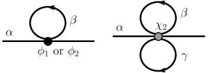
Figure 2: Hartree diagrams for the self-energy built from Eqs. (14) and (17). The full dots (resp. black and grey) indicate vertices with four or six external lines. $\alpha$, $\beta$ and $\gamma$ denote spins.

Therefore they can be incorporated into the elastic expression (23) where the phase shift is now given by Eq. (3) with $\delta n(\varepsilon)=f(\varepsilon,T)-\theta(\varepsilon_{F}-\varepsilon)$. More precisely, since $\sum_{\varepsilon}\delta n(\varepsilon)=0$ and $\sum_{\varepsilon}\varepsilon\,\delta n(\varepsilon)=(\pi T)^{2}/6$, the phase shift (3) simplifies to

$$\delta(\varepsilon,T)=\delta_{\rm el}(\varepsilon)-\frac{(N-1)\phi_{2}}{T_{K}^{2}}\frac{(\pi T)^{2}}{12},$$ (24)

where only the $\phi_{2}$ coupling survives. The last diagram to consider is shown Fig. 3.

Figure 3: Second order contribution to the self-energy corresponding to inelastic collisions.

It describes relaxation due to electron inelastic collisions nozieres1974a ; nozieres1974b+nozieres1978 . Its calculation follows from Ref. affleck1993 leading to

$$\Sigma^{R}_{1,{\rm in}}(\varepsilon,T)=-\frac{i\,e^{2i\delta_{0}}}{4}(N-1)\left(\frac{\phi_{1}}{T_{K}}\right)^{2}\left[\varepsilon^{2}+(\pi T)^{2}\right],$$ (25)

where the $N-1$ factor comes from the intermediate spin summation.

To summarize our findings, the self-energy $\Sigma_{1}^{R}=\Sigma^{R}_{1,{\rm el}}+\Sigma^{R}_{1,{\rm in}}$ is the sum of inelastic (25) and elastic (23) contributions with the phase shift (24). From this result, the transport observables (22) can be determined at low energy for any $N$. Instead, we start at this point to investigate the large $N$ limit keeping only the first order $1/N$ corrections. Hence we approximate $\sin\delta_{0}\simeq\pi/N$ and $\cos 2\delta_{0}\simeq 1$. Expanding the single-particle lifetime at low energy, we find

$$\begin{split}&\frac{\tau(\varepsilon,T)}{\tau(0,0)}=1-\frac{2\bar{\alpha}_{1}\varepsilon}{T_{K}}+\frac{3\bar{\alpha}_{1}^{2}\varepsilon^{2}}{T_{K}^{2}}\\[2.84526pt] &-\frac{2\bar{\alpha}_{2}}{T_{K}^{2}}\left[\varepsilon^{2}-\frac{(\pi T)^{2}}{3}\right]-\frac{\bar{\alpha}_{1}^{2}}{T_{K}^{2}}\frac{1}{2N}[\varepsilon^{2}+(\pi T)^{2}],\end{split}$$ (26)

with the renormalized coefficients $\bar{\alpha}_{1,2}=(N/\pi)\alpha_{1,2}$. Before proceeding further, let us discuss the normalization of $\alpha_{1}$. The Kondo temperatures in the FL theory and in the large $N$ approach of Ref. houghton1987 coincide if a single observable is matched between the two models, for instance the zero temperature magnetic susceptibility. In the FL theory, it reads nozieres1974a ; nozieres1974b+nozieres1978 ; nozieres1980

$$\chi_{0}=\frac{N\alpha_{1}}{N-1}\frac{N(N^{2}-1)}{12}\frac{(g\mu_{B})^{2}}{\pi T_{K}},$$ (27)

whereas $\frac{1}{3}(g\mu_{B})^{2}J(J+1)/T_{K}$ is the definition given in Ref. houghton1987 . $J$ is the angular momentum and the impurity model has $SU(2J+1)$ symmetry. A common Kondo temperature $T_{K}$ is thus achieved with $\bar{\alpha_{1}}=1-1/N$.

The conductance (22) is readily obtained from the electron lifetime (26) with the result

$$\begin{split}\frac{\sigma(T)}{\sigma(0)}&=1+\left(\frac{\pi T}{T_{K}}\right)^{2}\left[\bar{\alpha}_{1}^{2}\left(1-\frac{2}{3N}\right)+{\cal O}\left(\frac{1}{N^{2}}\right)\right]\\[2.84526pt] &=1+\left(\frac{\pi T}{T_{K}}\right)^{2}\left[1-\frac{8}{3N}+{\cal O}\left(\frac{1}{N^{2}}\right)\right],\end{split}$$ (28)

in full agreement with Ref. houghton1987 . This agreement confirms that the two procedures, namely the FL theory expanded at large $N$ on one side, and the large $N$ approach expanded at low energy on the other side, indeed correspond to the same physical limit. Nevertheless it does not help us to validate the new dimension-$4$ FL corrections since $\bar{\alpha}_{2}$ disappears from the final result (28).

The situation is markedly different for the Lorentz ratio (22). Using

$$\int_{-\infty}^{-\infty}d\varepsilon\,\varepsilon^{4}\left(-\frac{\partial f(\varepsilon,T)}{\partial\varepsilon}\right)=\frac{7(\pi T)^{4}}{15},$$

and the electron lifetime (26), we obtain, up to ${\cal O}(1/N)$,

$$\frac{L(T)}{L_{0}}=1+\frac{8}{15}\left(\frac{\pi T}{T_{K}}\right)^{2}\left[\frac{7}{2}\bar{\alpha}_{1}^{2}-4\bar{\alpha}_{2}^{2}-\frac{1}{N}\right],$$ (29)

where $\bar{\alpha}_{2}$ is explicitly present. The large $N$ expansion of the universal ratio (19) (with $m=1$),

$$\frac{\alpha_{2}}{\alpha_{1}^{2}}\simeq\frac{N}{\pi}\,\left(1+\frac{2\ln 2-1}{N}\right),$$ (30)

is introduced in Eq.(29), leading eventually to

$$\frac{L(T)}{L_{0}}=1-\frac{4}{15}\left(\frac{\pi T}{T_{K}}\right)^{2}\left[1+\frac{8}{N}(2\ln 2-1)\right].$$ (31)

Again there is full agreement with Ref.houghton1987 .

One conclusion that can be drawn from these results is that our extension of the FL theory satisfies a stringent test imposed by the large $N$ approach. We can also be confident in our theory and reverse the perspective with the following conclusion: we have checked on representative observables that the $1/N$ expansion of Read and Newns is correct at low energy.

VI Conclusions

In the case of a generalized SU(N) symmetry for the impurity away from half-filling, the Kondo resonance is centered off the Fermi energy. One consequence is that observables like the resistivity in magnetic alloys, or the current and the noise in quantum dots, require at low energy the introduction of the next-to-leading order correction around the Fermi liquid fixed point. Two possible reasonings have been employed in this work to identify the new Fermi liquid corrections. In a first approach, the Landau expansion of the phase shift has been pushed to the next order. The coefficients of the three resulting new contributions have further been related by using the floating argument. Physically, the floating expresses the fact that the Kondo resonance is built only by the distribution of conduction electron and follows its Fermi singularity.

In a second approach, we have proposed a single operator, cubic in the spin currents, and which remains invariant over SU(N) rotations. This operator resembles the cubic Casimir invariant of the SU(N) Lie algebra. Performing point splitting, we have recovered the same three processes with the same relation between their coupling constants. In fact, the reduction of coupling constants can be assigned to a common physical origin: the quenching of charge excitation on the impurity. In the first approach, the only fixed absolute energy reference that the Kondo resonance might depend on, is the single-particle energy level. It is effectively pushed to infinity in the Kondo limit which allows to develop the floating argument. In the second approach, the fact that charge excitations are frozen imposes that our cubic operator involves only spin currents.

Next the ratio between the leading and the next-to-leading order corrections has been determined by comparison with the exact solution for the free energy. This reduces further the number of coupling constants to a single one which is essentially the inverse of the Kondo temperature. Finally, the large $N$ regime of our theory has been shown to coincide exactly with field theoretical large $N$ predictions, thereby comforting our analysis.

Let us conclude by noting some consequences for experiments (experiments in alloys with magnetic impurities are reviewed in Ref. schlottmann1989 with a comparison to exact Bethe ansatz results). The subtleties of this work do not apply to the ordinary spin-$1/2$ Kondo effect with SU(2) symmetry since our novel corrections all vanish in that case (and for a half-filled dot in general). However, for experiments probing a possible SU(4) Kondo effect, the ingredients presented here are necessary to determine the low energy properties of the model.

The author is grateful to M. Bauer, M.-S. Choi, A. A. Clerk, K. Le Hur, T. Kontos, X. Leyronas and N. Regnault for interesting discussions.

References

- (1) A. Hewson, The Kondo Problem to Heavy Fermions (Cambridge University Press, Cambridge 1993).
- (2) A. Oguri, Phys. Rev. B 64 153305 (2001); Y. Meir and A. Golub, Phys. Rev. Lett 88 116802 (2002); A. Rosch, J. Paaske, J. Kroha, P. Wölfle, Phys. Rev. Lett 90 076804 (2003); S. Kehrein, Phys. Rev. Lett 95 056602 (2005); P. Mehta, N. Andrei, Phys. Rev. Lett 96 216802 (2006); F. B. Anders, Phys. Rev. Lett 101 066804 (2008).
- (3) P. Nozières, J. Low Temp. Phys. 17 31 (1974).
- (4) P. Nozières, in Proceedings of the 14th International Conference on Low Temperature Physics edited by M. Krasius and M. Vuorio (North Holland, Amsterdam, 1974) pp. 339-374; P. Nozières, J. Physique 39 1117 (1978).
- (5) K.G. Wilson, Rev. Mod. Phys. 47 773 (1975).
- (6) I. Affleck, Nucl. Phys. B 336 517 (1990).
- (7) I. Affleck and A. W. W. Ludwig, Phys. Rev. B 48 7297 (1993).
- (8) I. Affleck, A. W. W. Ludwig, Nucl. Phys. B 352 849 (1991).
- (9) F. Lesage, H. Saleur, Phys. Rev. Lett 82 4540 (1999); F. Lesage, H. Saleur, Nucl. Phys. B 546 585 (1999).
- (10) K. Yosida, K. Yamada, Progr. Theoret. Phys. Suppl. 46 244 (1970); K. Yamada, Progr. Theoret. Phys. 53 970 (1975); K. Yosida, K. Yamada, Progr. Theoret. Phys. 53 1286 (1975); K. Yamada, Progr. Theoret. Phys. 54 316 (1975).
- (11) A.C. Hewson, Adv. Phys. 43 543 (1994).
- (12) P. Nozières, A. Blandin, J. Phys. (Paris) 41 193 (1980).
- (13) B. Coqblin, J.R. Schrieffer, Phys. Rev. 185 847 (1969).
- (14) N. Andrei, K. Furuya, J.H. Lowenstein, Rev. Mod. Phys. 55 331 (1983); A.M. Tsvelik, P.B. Wiegmann, J. Phys. C 15 1707 (1982); J.W. Rasul, in Valence Instabilities edited by P. Wachter and H. Boppart (North Holland, Amsterdam, 1982) p. 49.
- (15) P. Schlottmann, Z. Phys. B 49 109 (1982); A.M. Tsvelik, P.B. Wiegmann, Adv. Phys. 32 453 (1983).
- (16) S. Sasaki, S. Amaha, N. Asakawa, M. Eto, and S. Tarucha, 93 017205 (2004).
- (17) P. Jarillo-Herrero, J. Kong, H. S. van der Zant, C. Dekker, L. P. Kouwenhoven, S. D. Franceschi, Nature(London) 434 484 (2005); A. Makarovski, A. Zhukov, J. Liu, G. Finkelstein, Phys. Rev. B 75 241407 (2007); A. Makarovski, J. Liu, G. Finkelstein, Phys. Rev. Lett 99 066801 (2007).
- (18) T. Delattre et al., Nature Physics 5 208 (2009).
- (19) D.C. Langreth, Phys. Rev. 150 516 (1966).
- (20) V.V. Bazhanov, S.L. Lukyanov, A.M. Tsvelik, Phys. Rev. B 68 094427 (2003).
- (21) L.I. Glazman and M. Pustilnik, in Nanophysics: Coherence and Transport edited by H. Bouchiat et al. (Elsevier 2005) pp. 427-478, arXiv:cond-mat/0501007.
- (22) P. Vitushinsky, A. A. Clerk, and K. Le Hur, Phys. Rev. Lett 100 036603 (2008).
- (23) K. Le Hur, P. Simon, and D. Loss, Phys. Rev. B 75 035332 (2007).
- (24) C. Mora, X. Leyronas, N. Regnault, Phys. Rev. Lett 100 036604 (2008).
- (25) C. Mora, X. Leyronas, N. Regnault, Phys. Rev. Lett 102 139902 (2009).
- (26) D. M. Newns, N. Read, Adv. Phys. 36 799 (1987).
- (27) V. T. Rajan, Phys. Rev. Lett 51 308 (1983).
- (28) J. Kondo, Progr. Theoret. Phys. 32 37 (1964).
- (29) K. D. Schotte, Z. Physik 230 99 (1970).
- (30) J. A. de Azcárraga, A. J. Macfarlane, A. J. Mountain, J. C. Pérez Bueno, Nucl. Phys. B 510 657 (1998).
- (31) D. Bensimon, A. Jerez, M. Lavagna, Phys. Rev. B 73 224445 (2006).
- (32) A. Klein, J. Math. Phys. 4 1283 (1963).
- (33) E. Sela, Y. Oreg, F. von Oppen, and J. Koch, Phys. Rev. Lett 97 086601 (2006); A. Golub, Phys. Rev. B 73 233310 (2006); A.O. Gogolin and A. Komnik, Phys. Rev. Lett 97 016602 (2006).
- (34) P. Coleman, Phys. Rev. B 29 3035 (1984).
- (35) A. Houghton, N. Read, H. Won, Phys. Rev. B 35 5123 (1987).
- (36) P. Schlottmann, Phys. Rep. 181 1 (1989).