Harmonic functions on hyperbolic graphs

Abstract.

We consider admissible random walks on hyperbolic graphs. For a given harmonic function on such a graph, we prove that asymptotic properties of non-tangential boundedness and non-tangential convergence are almost everywhere equivalent. The proof is inspired by the works of F. Mouton in the cases of Riemannian manifolds of pinched negative curvature and infinite trees. It involves geometric and probabilitistic methods.

1. Introduction

The study of non-tangential convergence of harmonic functions began in 1906 with P. Fatou [Fat06], who showed that a given positive harmonic function on the unit disc of $\mathbb{R}^{2}$ admits at almost all points of the unit circle a non-tangential limit. The same is true in many general cases: euclidean half-spaces, trees ([Car72]), free groups ([Der75]), Riemannian manifolds of pinched negative curvature ([AnS85], [Anc87]) and Gromov hyperbolic graphs ([Anc90]). One is thus naturaly led to the study of cases where the harmonic function is not necessarily positive. Fatou’s conclusion is no longer true in this more general case, and several authors have made attempts to give criteria for the harmonic function to admit non-tangential limit at a point of the boundary. In the case of the euclidean half space ${\mathbb{R}^{n}\times\mathbb{R}_{+}^{*}}$, A.P. Calderòn and E.M. Stein ([Cal50a], [Cal50b], [Ste61]) proved that for a harmonic function $u$, the following three properties are equivalent for almost all point $\theta$ of the boundary:

• the function $u$ is non-tangentially convergent at $\theta$

• the function $u$ is non-tangentially bounded at $\theta$

• the area integral $\intop_{\Gamma_{\theta}}|\nabla u(x,y)|^{2}y^{1-n}dxdy$ is finite (for all $\Gamma^{\theta}$ where $\Gamma^{\theta}$ is a non-tangential cone).

In 1978, using probabilistic methods, J. Brossard proved the same result [Bro78]. Shortly after, A. Koranyi remarked that hyperbolic spaces provide a more natural setting for this study. Indeed, several notions have simpler expressions in this case. For instance the boundary becomes an ideal one, non-tangential cones become tubular neighborhoods of geodesic rays. Following this remark, F. Mouton proved in 1994 an analogous result for harmonic functions on Riemannian manifolds of pinched negative curvature [Mou94], and in 2000 for harmonic functions on trees [Mou00]. We prove here a partial analogue for hyperbolic graphs: for a harmonic function (the notion of harmonicity is here relative to a random walk on the graph), non-tangential convergence is almost everywhere equivalent to non-tangential boundedness.

We introduce in section 2 the notions of random walks and harmonic functions on hyperbolic graphs and in section 3 the boundary at infinity, which enables us to state our main result in section 4. Section 5 is devoted to the conditioning of the random walk to exit at a fixed point of the boundary and to the proof of a stochastic result. In order to prove the non-tangential convergence criterion, we state geometric lemmas in section 6. We then prove the main result in section 7.

2. Harmonic functions on hyperbolic graphs

We shall briefly introduce the notions of hyperbolic graphs, random walks, harmonic functions and Green functions. The reader can refer to [Woe00] for more details.

2.1. Hyperbolic graphs

Gromov hyperbolicity was introduced in the 80’s by M. Gromov [Gro81]. One way to define it is the following:

Definition 2.1.

On a metric space $(X,d)$, one defines the Gromov product of two points $x,y\in X$ with respect to $o\in X$ by

$$(x,y)_{o}=\frac{1}{2}[d(x,o)+d(y,o)-d(x,y)].$$

For a real $\delta\geq 0$, a metric space $X$ is said to be $\delta$-hyperbolic if for all $x,y,z,o\in X$,

$$(x,z)_{o}\geq\min\{(x,y)_{o},(y,z)_{o}\}-\delta.$$

A metric space $(X,d)$ is geodesic if for every pair of points $x$ and $y$ in $X$, there is a geodesic segment (not necessarily unique) joining $x$ to $y$ in $X$ ( i.e. an isometric embedding of the real interval $[0,d(x,y)]$ into $X$ which sends $0$ to $x$ and $d(x,y)$ to $y$).

The definition of Gromov hyperbolicity makes sense in all metric spaces. However, it has a nice geometric interpretation when the space is geodesic. A geodesic triangle consists of three points $x,y,z\in X$ together with geodesic segments $\alpha$, $\beta$, $\gamma$ (respectively from $y$ to $z$, $z$ to $x$ and $x$ to $y$) called the sides. A triangle is called $\eta$-thin for a real $\eta\geq 0$ if every point of a side is at distance at most $\eta$ from the union of the other two sides. If a geodesic metric space $X$ is $\delta$-hyperbolic, then every geodesic triangle in $X$ is $4\delta$-thin. Remark that the converse also holds, if every geodesic triangle in $X$ is $\eta$-thin, then $X$ is $3\eta$-hyperbolic. The reader can keep in mind that the Gromov product $(x,y)_{o}$ can be seen as a rough measure of the distance between $o$ and a geodesic segment joining $x$ and $y$ (see [GdlH90]). Precisely, if $X$ is $\delta$-hyperbolic and $\gamma$ is a geodesic segment from $x$ to $y$, then

(2.1) $$d(o,\gamma)-2\delta\leq(x,y)_{o}\leq d(o,\gamma).$$

Let $S$ be a countable graph, that is, it is a countable set $S$ equipped with a reflexive symmetric relation $Z\subset S\times S$. A path from $x$ to $y$ in $S$ is a sequence $[x=x_{0},x_{1},...,x_{k}=y]$ such that for all indices $i$, $(x_{i-1},x_{i})\in Z$. The integer $k$ is the length of the path. We shall always assume that $S$ is connected, i.e. that for every pair $x$, $y$ in $S$, there is a path from $x$ to $y$. The graph $S$ carries an integer-valued metric: $d(x,y)$ is the minimum among all the lengths of the paths from $x$ to $y$. If the metric space $(S,d)$ is $\delta$-hyperbolic for a real $\delta\geq 0$, we will say that the graph $S$ is hyperbolic. Typical examples are provided by trees and Cayley graphs of certain groups. If the Cayley graph of a finitely generated group associated to one finite generating set is hyperbolic, then the Cayley graph associated to every finite generating set is hyperbolic and the group is called Gromov hyperbolic.

We will focus our interest on coercive graphs satisfying the geometric assumption (GRBD).

Definition 2.2.

A graph $S$ is called coercive if there is some positive $\alpha$ such that the following Poincaré-Sobolev inequality holds:

$$\sum_{(x,y)\in Z}|u(y)-u(x)|^{2}\geq\alpha\cdot||u||_{2}^{2}$$

for all $u:S\to\mathbb{R}$ with finite support.

One can verify that the coercivity of $S$ is equivalent to an isoperimetric inequality [Anc90]. An example of coecive graph is given by a discrete approximation of the hyperbolic ball: denote by $B$ the unit ball of $\mathbb{R}^{n}$ equipped with the hyperbolic metric $d_{h}$. Let $S\subset B$ be such that for all $x\in B$, $d_{h}(x,S)\leq c_{1}$ and for all $x,y\in S$, $d_{h}(x,y)\geq c_{2}$. Equip $S$ with the relation $(x,y)\in Z$ iff $d_{h}(x,y)\leq 3c_{1}$. Then, $S$ is a coercive graph, whose metric is uniformly equivalent to $d_{h}$.

Definition 2.3.

A graph $S$ satisfies the Geodesic Ray at Bounded Distance (GRBD) assumption if, given a base point $o$, there is a constant $K\geq 0$ with the property that every point in the graph is at distance at most $K$ from a geodesic ray starting from $o$.

This assumption will be used in the proof of lemma 6.4. It is satisfied for instance by geodesically complete graphs (any two points in the graph can be joined by a geodesic line) and by Cayley graphs of hyperbolic groups. Indeed, assume that $S$ is a Cayley graph of a hyperbolic group and denote by $\delta$ a hyperbolicity constant of $S$. Let $x\in S$. Choose two arbitrary points $\xi_{1},\xi_{2}\in\partial S$ and a geodesic joining them, which exists by visibility (see [GdlH90]). Up to translation, one can assume without loss of generality that it contains $x$. Let $\gamma_{1}$ denote a geodesic ray from $o$ to $\xi_{1}$ and $\gamma_{2}$ a geodesic ray from $o$ to $\xi_{2}$. Because all triangles are $4\delta$-thin, $x$ is at distance at most $4\delta$ from one of the two geodesic rays.

2.2. Random walks

Let $S$ be a graph and $d$ the corresponding distance. Let us choose a (transition) function $p:S\times S\to\mathbb{R}^{+}$. This function $p$ is markovian (resp. submarkovian) if for all $x\in S$, $\sum_{y\in X}p(x,y)=1$ (resp. $\sum_{y\in X}p(x,y)\leq 1$) and admissible in the sense of A. Ancona ([Anc88]) if the following relations hold:

1. $\exists c_{0}>0,\exists\ell\in\mathbb{N}^{*}$ such that $\forall x,y\in S$, $d(x,y)\leq 1\Rightarrow\sum_{0\leq j\leq\ell}p^{j}(x,y)\geq c_{0}$,

2. $\exists m_{1}\in\mathbb{N}^{*}$ such that $\forall x,y\in S$, $p(x,y)>0\Rightarrow d(x,y)\leq m_{1}$.

The admissible conditions are geometric adaptedness properties of the transition function $p$ to the structure of the graph $S$.

Remark that the adjoint kernel $p^{*}(x,y)=p(y,x)$ and $p+tI$, $t\geq 0$ are also admissible. In the following, we will always assume $p$ to be markovian. We define the $p$-random walk on $S$ as the Markov chain with state space $S$ and transition probabilities $p(x,y)$, $x,y\in S$. It is given by a family of random variables $(X_{n})_{n\in\mathbb{N}}$ on $S$ where $X_{n}$ is the position at time $n$. We can choose the probability space to be the space $\Omega=\mathcal{C}(\mathbb{N},S)$ of all infinite paths (then, $X_{n}(\omega)=\omega(n)$), equipped with the $\sigma$-algebra arising from the countable product of $\mathcal{P}(S)$. We will denote by $(\mathbb{P}_{z})_{z\in S}$ the law of this random walk, where $\mathbb{P}_{z}$ is the probability obtained when the walk starts from $z$ and by $\mathcal{F}_{n}$ the $\sigma$-algebra generated by $X_{i},i\leq n$.

We can now state a classical property which will be useful in the following. For an almost surely finite stopping time $T$, we denote by $\Theta^{T}$ the map: $\Theta^{T}(\omega)=\omega(\cdot+T(\omega))$.

Lemma 2.4 (Strong Markov property).

For a non-negative random variable $F$ on $\Omega$ and an almost surely finite stopping time $T$ one has

$$\mathbb{E}_{x}[F\circ\Theta^{T}|\mathcal{F}_{T}]=u_{F}(X_{T})\text{ where }u_{F}(y)=\mathbb{E}_{y}[F].$$

2.3. Harmonic functions and the Green function

We associate to the random walk a Laplace operator $\Delta$ which acts on functions $f:S\to\mathbb{R}$ by

$$\Delta f(x)=\mathbb{E}_{x}[f(X_{1})]-f(x)=\sum_{y\in S}p(x,y)f(y)-f(x).$$

A function $f$ is said to be harmonic if $\Delta f=0$ and superharmonic if $\Delta f\leq 0$.

The Green function associated to the random walk is thus defined on $S\times S$ by

$$G(x,y):=\sum_{n=0}^{\infty}\mathbb{P}_{x}[X_{n}=y]=\mathbb{E}_{x}\left[\sum_{n=0}^{\infty}\mathbf{1}_{\{X_{n}=y\}}\right].$$

It can be seen by the Markov property that the function $G(\cdot,y)$ is harmonic on $S\setminus\{y\}$ and superharmonic on $S$.

Lemma 2.5 (Martingale property).

Let $z$ be a point of $S$ and $f$ be a function on $S$. Then, the sequence of random variables

$$M_{n}=f(X_{n})-\sum_{k=0}^{n-1}\Delta f(X_{k})$$

is a $(\mathcal{F}_{n})$-martingale for the probability $\mathbb{P}_{z}$. In particular, $(f(X_{n}))_{n}$ is a martingale if $f$ is harmonic.

Denote by $G^{t}$ the Green kernel of the admissible transition function $p+tI$. A. Ancona introduced in [Anc88] the condition:

$$\text{(*) there exists }\varepsilon>0,\text{ such that }G^{\varepsilon}\text{ is finite.}$$

This hypothesis implies in particular that the random walk is transient and that some Harnack inequalities hold at infinity. In [Anc90], A. Ancona proves the following proposition:

Proposition 2.6 (Ancona).

If $S$ is coercive, every admissible kernel $p$ on $S$ such that $p$ and $p^{*}$ are submarkovian satisfies condition (*) and admits a Green function $G$ such that $G(x,y)\leq C\cdot\exp(-\beta d(x,y))$ for some positive constants $C,\beta$.

Remark 2.7.

the assumption in the proposition is satisfied by non-amenable, finitely generated groups $\Gamma$ with an admissible probability measure $\nu$ on $\Gamma$ ($p(x,y)=\nu(\{x^{-1}y\})$).

3. Boundary at infinity

Since we are interested in non-tangential convergence, we need a notion of boundary. In fact, we will focus our interests on two types of boundaries: the geometric boundary and the Martin one. To define them, we will need to fix a base point $o\in S$, but the compactifications below do not depend on the choice of $o$.

• The geometric boundary $\partial S$. Assume $S$ to be a hyperbolic graph. Let us denote by $E$ the set of sequences $(x_{i})_{i}$ in $S$ such that $\lim_{i,j\to\infty}(x_{i},x_{j})_{o}=+\infty$ and by $\partial S=E/\mathcal{R}$ the set obtained by factoring $E$ with respect to the equivalence relation: $(x_{i})_{i}\mathcal{R}(y_{j})_{j}$ iff $\lim_{i,j\to\infty}(x_{i},y_{j})_{o}=+\infty$. An equivalent way to describe $\partial S$ is via equivalence of geodesic rays (see [GdlH90]): two geodesic rays $\gamma_{1}$ and $\gamma_{2}$ are equivalent if $\liminf_{k\to\infty}d(\gamma_{1}(k),\gamma_{2}(\mathbb{N}))<+\infty$. One can extend the Gromov product to two points $x,y\in\partial S$ (resp. $x\in S$, $y\in\partial S$ or $x\in\partial S$, $y\in S$) with

  $$(x,y)_{o}=\sup\liminf_{i,j\to\infty}(x_{i},y_{j})_{o}\hskip 14.22636pt(\text{resp. }(x,y)_{o}=\sup\liminf_{j\to\infty}(x,y_{j})_{o}),$$

  where the supremum is taken over all sequences $(x_{i})_{i}$ in the class of $x$ and $(y_{j})_{j}$ in the class of $y$. For a real $r>0$ and a point $x\in\partial S$, denote by $V_{r}(x)=\{y\in S\cup\partial S\,|\,(x,y)_{o}\geq r\}$. We equip $S\cup\partial S$ with the unique topology containing open sets of $S$ and admitting the sets $V_{r}(x)$ with $r\in\mathbb{Q}^{+}$ as neighborhood base at any $x\in\partial S$. It provides a compactification $\tilde{S}$ of $S$ (that is a compact Hausdorff space with countable base of the topology such that $S$ is open and dense in $\tilde{S}$). The compactification $\tilde{S}$ can also be obtained as the completion of $S$ for a good choice of a metric on $S$ (see [Woe00]).

• The Martin boundary. Assume the random walk to be transient. One defines the Martin kernel by $K(x,y)=\frac{G(x,y)}{G(o,y)}$. The Martin compactification $\hat{S}$ is the unique smallest compactification of $S$ for which all kernels $K(x,.)$, $x\in S$, extend continuously. The Martin boundary is $\hat{S}\setminus S$. A sequence $(y_{i})_{i}\in S^{\mathbb{N}}$ converges to the Martin boundary if $d(o,y_{i})\to\infty$ and $(K(.,y_{i}))_{i}$ converges pointwise. Two such sequences are equivalent if their limits coincide at each point of $S$. The Martin boundary allows us to represent non-negative harmonic functions by non-negative measures on this boundary (see [Woe00]).

Results by A. Ancona ([Anc90]) imply that in the case of a hyperbolic graph with an admissible transition function $p$ on $S$ satisfying condition (*), these two compactifications coincide. In the following, we will assume that $S$ is a coercive hyperbolic graph and $p$ be an admissible markovian transition function on $S$ such that $p^{*}$ is submarkovian. The above two boundaries of $S$ thus coincide and we shall denote it by $\partial S$. There is a $\partial S$-valued random variable $X_{\infty}$ such that the random walk $(X_{n})_{n}$ converges $\mathbb{P}_{z}$-almost surely to $X_{\infty}$ for all $z\in S$ (see [Woe00]). When dealing with harmonic functions and random walks, there is a natural family of measures on $\partial S$ called the harmonic measures $\mu_{z},z\in S$. The measure $\mu_{z}$ is the distribution of the random variable $X_{\infty}$ when the walk starts from $z$. Different measures $\mu_{z}$ are equivalent, so we can define a notion of $\mu$-negligeability. Their Radon-Nykodim derivatives are given by

$$\frac{d\mu_{y}}{d\mu_{x}}(\theta)=\lim_{z\to\theta}\frac{G(y,z)}{G(x,z)}.$$

These measures allow to represent bounded harmonic functions by the Poisson formula (see [Woe00] and lemma 5.3).

4. Main result

Setting: We fix now a coercive hyperbolic graph $S$ satisfying (GRBD) and an admissible markovian transition function $p$ on $S$ such that $p^{*}$ is submarkovian.

Let $d$ be the canonical distance on $S$ , $\delta\geq 0$ the hyperbolicity constant, $c_{0}$, $\ell$ and $m_{1}$ the admissibility constants and $o\in S$ a base point. After possibly enlarging it, we will assume that $\delta$ is an integer strictly bigger than 3.

Let us now define the non-tangential notions. If $c>0$ and $\theta\in\partial S$, let us denote by

$$\Gamma_{c}^{\theta}:=\{x\in S\,|\,\exists\gamma\text{ a geodesic ray from }o\text{ to }\theta\text{ such that }d(x,\gamma)<c\}$$

the non-tangential tube of radius $c$ and vertex $\theta$. A function $u$ converges non-tangentially at $\theta$ if, for all $c>0$, $u(x)$ has a limit as $x$ goes to $\theta$ in $\Gamma_{c}^{\theta}$. In the same manner, the function $u$ is non-tangentially bounded at $\theta$ if, for all $c>0$, $u$ is bounded on $\Gamma_{c}^{\theta}$. Remark that these non-tangential notions do not depend on $o$, due to the alternative definition of $\partial S$ by geodesic rays.

We can now state our main result.

Theorem 4.1.

In the setting above, for a harmonic function $u$, the following two properties are equivalent for $\mu$-almost all $\theta\in\partial S$:

1. the function $u$ converges non-tangentially at $\theta$,

2. the function $u$ is non-tangentially bounded at $\theta$.

Denote

$$\mathcal{L}_{c}=\{\theta\in\partial S\,|\,\lim_{\stackrel{{\scriptstyle x\in\Gamma_{c}^{\theta}}}{{x\to\theta}}}u(x)\text{ exists and is finite}\},$$

$$\mathcal{N}_{c}=\{\theta\in\partial S\,|\,N_{c}^{\theta}(u)<\infty\}\text{ where }N_{c}^{\theta}(u)=\sup_{x\in\Gamma_{c}^{\theta}}|u(x)|$$

and observe that

$$\mathcal{L}=\bigcap_{c>0}\mathcal{L}_{c}\hskip 14.22636pt\text{ and }\hskip 14.22636pt\mathcal{N}=\bigcap_{c>0}\mathcal{N}_{c}.$$

The theorem can be stated by: $\mathcal{N}\approx\mathcal{L}$, where $\approx$ means that the two sets differ by a $\mu$-negligeable set.

The proof of this result uses stochastic methods which will be explained in the next section.

5. Conditioning

By Doob’s h-processes, it is possible to condition the random walk to exit at a fixed point $\theta\in\partial S$ (see [Doo57] and [Dyn69]). The probability $\mathbb{P}_{z}^{\theta}$ on $\Omega$ thus obtained satisfies a strong Markow property and one has the following property:

Proposition 5.1.

Let $F$ be a non-negative random variable on $\Omega$. Then

$$\mathbb{E}_{z}[F]=\intop_{\partial S}\mathbb{E}_{z}^{\theta}[F]d\mu_{z}(\theta).$$

The probability $\mathbb{P}_{z}^{\theta}$ satisfies an asymptotic zero-one law: if an event $A$ is asymptotic (i.e. if it is invariant under the shift operator $\Theta$) then, for all $\theta\in\partial S$, the map $z\mapsto\mathbb{P}_{z}^{\theta}(A)$ is constant on $S$ and equals either $0$ or $1$. The reader can refer to [Mou94], [Bro78] and [Dur84] for more details.

As mentioned above, we shall use probabilistic methods. We shall therefore define stochastic analogues of non-tangential convergence and boundedness notions. Let $u$ be a harmonic function. Let $\widetilde{\mathcal{N}^{**}}$ be the set of trajectories $\omega$ such that $|u|$ is bounded on the thickened trajectory $\{y\in S|d(y,\omega)\leq m_{1}\}$:

$$\widetilde{\mathcal{N}^{**}}=\{\omega\in\Omega\,|\,\widetilde{N^{*}}(\omega)<+\infty\}\text{ where }\widetilde{N^{*}}(\omega)=\sup\{|u(y)|\,|\,y\in S,d(y,\omega)\leq m_{1}\}.$$

We also define the set

$$\mathcal{L}^{**}=\{\omega\in\Omega\,|\,\lim_{n\to\infty}u(X_{n}(\omega))\text{ exists and is finite}\}.$$

These two events are asymptotic, so by asymptotic zero-one law, quantities $\mathbb{P}_{z}^{\theta}(\widetilde{\mathcal{N}^{**}})$ and $\mathbb{P}_{z}^{\theta}(\mathcal{L}^{**})$ have values $0$ or $1$ and do not depend on $z$. We thus define the sets

$$\widetilde{\mathcal{N}^{*}}=\{\theta\in\partial S\,|\,\mathbb{P}_{o}^{\theta}(\widetilde{\mathcal{N}^{**}})=1\}\text{ and }\mathcal{L}^{*}=\{\theta\in\partial S\,|\,\mathbb{P}_{o}^{\theta}(\mathcal{L}^{**})=1\}.$$

We say that $u$ is stochastically bounded at $\theta\in\partial S$ if $\theta\in\widetilde{\mathcal{N}^{*}}$ and that $u$ converges stochastically at $\theta$ if $\theta\in\mathcal{L}^{*}$. For every $r\in\mathbb{R}$, the event $\{\omega\,|\,\lim_{n\to\infty}u(X_{n}(\omega))\leq r\}$ is asymptotic, thus if $\theta\in\mathcal{L}^{*}$, $\lim_{n\to\infty}u(X_{n})$ is $\mathbb{P}_{o}^{\theta}$-almost surely constant.

We now prove a stochastic analogue of our main result.

Proposition 5.2.

Given a harmonic function $u$, one has the $\mu$-almost inclusion

$$\widetilde{\mathcal{N}^{*}}\stackrel{{\scriptstyle\sim}}{{\subset}}\mathcal{L}^{*}.$$

Proof.

We will first prove the $\mathbb{P}_{o}$-almost inclusion $\widetilde{\mathcal{N}^{**}}\stackrel{{\scriptstyle\sim}}{{\subset}}\mathcal{L}^{**}$. For $m\in\mathbb{N}$, denote by $\widetilde{\mathcal{N}_{m}^{**}}$ the set of trajectories $\omega$ such that $|u|$ is bounded by $m$ on the thickened trajectory ${\{y\in S\,|\,d(y,\omega)\leq m_{1}\}}$. By countable union, it is sufficient to prove that for all $m$, ${\widetilde{\mathcal{N}_{m}^{**}}\stackrel{{\scriptstyle\sim}}{{\subset}}\mathcal{L}^{**}}$. Denote by $T_{m}$ the stopping time

$$T_{m}:=\inf\{n\geq 0\,|\,\max\{|u(y)|\,|\,y\in S,d(y,X_{n})\leq m_{1}\}>m\}.$$

Remark that $\widetilde{\mathcal{N}_{m}^{**}}=\{T_{m}=+\infty\}$. Since $u$ is harmonic, $(u(X_{n}))_{n\in\mathbb{N}}$ is a martingale for the probability $\mathbb{P}_{o}$ and thus $(u(X_{n\wedge T_{m}}))_{n}$ is a martingale too. With our choice of stopping time $T_{m}$, for all $n\in\mathbb{N}$, $|u(X_{n\wedge T_{m}})|\leq\max\{m,|u(X_{o})|\}$, which implies by the martingale theorem that the stopped martingale converges $\mathbb{P}_{o}$-almost surely. In particular, $(u(X_{n}))_{n}$ converges $\mathbb{P}_{o}$-almost surely on the event $\widetilde{\mathcal{N}_{m}^{**}}$. We thus proved that $\widetilde{\mathcal{N}_{m}^{**}}\stackrel{{\scriptstyle\sim}}{{\subset}}\mathcal{L}^{**}$ and since $\widetilde{\mathcal{N}^{**}}=\bigcup_{m}\widetilde{\mathcal{N}_{m}^{**}}$ we obtain that $\widetilde{\mathcal{N}^{**}}\stackrel{{\scriptstyle\sim}}{{\subset}}\mathcal{L}^{**}$.

Using proposition 5.1, we have

$$0=\mathbb{P}_{o}(\widetilde{\mathcal{N}^{**}}\setminus\mathcal{L}^{**})=\intop_{\partial S}\mathbb{P}_{o}^{\theta}(\widetilde{\mathcal{N}^{**}}\setminus\mathcal{L}^{**})d\mu_{o}(\theta).$$

Then, $\mathbb{P}_{o}^{\theta}(\widetilde{\mathcal{N}^{**}}\setminus\mathcal{L}^{**})=0$ for $\mu$-almost all $\theta\in\partial S$ and $\widetilde{\mathcal{N}^{*}}\stackrel{{\scriptstyle\sim}}{{\subset}}\mathcal{L}^{*}$. ∎

We end this section with the case of bounded harmonic functions ([Woe00], [Anc90]).

Lemma 5.3.

A bounded harmonic function $u$ on $S$ converges non-tangentially and stochastically for $\mu$-almost all point $\theta\in\partial S$ and the unique function $f\in L^{\infty}(\partial S,\mu)$ such that

$$u(x)=\intop_{\partial S}f(\theta)d\mu_{x}(\theta)=\mathbb{E}_{x}[f(X_{\infty})]$$

is $\mu$-a.e. the non-tangential and stochastic limit of $u$.

6. Geometric lemmas

We begin this section by showing that a hyperbolicity inequality holds for points on the boundary $\partial S$: for all $x,y,z\in S\cup\partial S$,

(6.1) $$(x,y)_{o}\geq\min\{(x,z)_{o},(y,z)_{o}\}-2\delta.$$

To see this, choose, for $\epsilon>0$, sequences in $S$ with $x_{i}\to x$, $y_{i}\to y$, $z_{i}\to z$ and $z_{i}^{\prime}\to z$ such that $\liminf_{i,j}(x_{i},z_{j})_{o}\geq(x,z)_{o}-\epsilon$ and $\liminf_{i,j}(z_{i}^{\prime},y_{j})_{o}\geq(z,y)_{o}-\epsilon$. Then, take $\liminf_{i,j}$ through $(x_{i},y_{j})_{o}\geq\min\{(x_{i},z_{j})_{o},(z_{j},z_{i}^{\prime})_{o},(z_{i}^{\prime},y_{j})_{o}\}-2\delta$ (note that $\liminf_{i,j}(z_{j},z_{i}^{\prime})_{o}=+\infty$).

We will also need the fact that for all $x\in S$, $\xi\in\partial S$, and all geodesic ray $\gamma$ from $o$ to $\xi$,

(6.2) $$d(x,\gamma)-2\delta\leq(o,\xi)_{x}\leq d(x,\gamma)+2\delta.$$

By inequality (2.1), for all $i$, $d(x,\gamma($⟦$0,i$ ⟧$))-2\delta\leq(o,\gamma(i))_{x}\leq d(x,\gamma($⟦$0,i$ ⟧$))$. Since $d(x,\gamma(i))\to\infty$, for $i$ large enough, $d(x,\gamma($⟦$0,i$ ⟧$))=d(x,\gamma)$ and hence for $i$ large enough,

$$d(x,\gamma)-2\delta\leq(o,\gamma(i))_{x}\leq d(x,\gamma).$$

Combining this inequality with the fact that if $(\xi_{i})_{i}$ is a sequence such that $\xi_{i}\to\xi$, thus $(o,\xi)_{x}-2\delta\leq\liminf_{i}(o,\xi_{i})_{x}\leq(o,\xi)_{x}$ (see [Bri99]), we obtain inequality (6.2).

Using the hyperbolicity of the graph, we shall prove two lemmas, and deduce three corollaries. In order to prove one of these lemmas (lemma 6.3), we shall need some Harnack inequalities (see [Anc88] and [Anc90]):

Theorem 6.1 (Harnack inequality).

Let $u$ be a non-negative superharmonic function. For all $x,y\in S$,

$$\left(\frac{c_{0}}{\ell}\right)^{d(x,y)}u(y)\leq u(x)\leq\left(\frac{\ell}{c_{0}}\right)^{d(x,y)}u(y).$$

The following theorem is a version of the so-called Harnack inequality at infinity of A. Ancona.

Theorem 6.2 (submultiplicativity of the Green function).

For any $r>0$, there exists a constant $C=C(r)$ such that, for all $x,z\in S$ and all $y\in S$ at distance at most $r$ from any geodesic segment between $x$ and $z$,

$$G(x,z)\leq C\cdot G(x,y)G(y,z).$$

We can now state the geometric lemmas. They will be of central importance in the proof of the main result (theorem 4.1).

Lemma 6.3.

Given $\alpha>0$, there exists a constant $C>0$ such that, for all point $x\in S$ and all $\theta\in\partial S$,

$$\mu_{x}(\{\xi\in\partial S\,|\,(\xi,\theta)_{x}\geq\alpha\})\geq C.$$

Proof.

First, we will show that there exists $N=N(\alpha)>0$ such that for all $x\in S$, all $\theta\in\partial S$ and all $y$ on a geodesic from $x$ to $\theta$ with $d(x,y)\geq N$, we have

$$\mu_{y}(A_{x,\alpha}^{\theta})>\frac{1}{2}$$

where

$$A_{x,\alpha}^{\theta}:=\{\xi\in\partial S\,|\,(\xi,\theta)_{x}\geq\alpha\}.$$

We have

$$\mu_{y}(\partial S\setminus A_{x,\alpha}^{\theta})=\intop_{\partial S\setminus A_{x,\alpha}^{\theta}}\frac{d\mu_{y}}{d\mu_{x}}(\xi)d\mu_{x}(\xi)$$

and

$$\frac{d\mu_{y}}{d\mu_{x}}(\xi)=\lim_{z\to\xi}\frac{G(y,z)}{G(x,z)}.$$

Let $\xi\in\partial S\setminus A_{x,\alpha}^{\theta}$. Denote by $\gamma$ a geodesic ray from $x$ to $\xi$, by $x_{j}=\gamma(4j\delta)$ and by $V_{j}$ the closure in $S\cup\partial S$ of $\{z\in S\,|\,(z,x_{j})_{x}>d(x,x_{j})-3\delta\}$.

We claim that there exist $j,N_{1}\in\mathbb{N}$ depending only on $\alpha$ such that if $y$ is on a geodesic from $x$ to $\theta$ and $d(x,y)\geq N_{1}$, then $y\notin V_{j}$ (see figure 1). Indeed, choose $j$ such that $d(x,x_{j})-3\delta=4j\delta-3\delta>\alpha+4\delta$. By the hyperbolicity inequality (6.1),

Figure 1. Lemma 6.3

$$\alpha>(\xi,\theta)_{x}\geq\min\{(\xi,y)_{x},(y,\theta)_{x}\}-2\delta$$

and if $y$ is on a geodesic ray from $x$ to $\theta$, there exists $N_{1}$ depending only on $\alpha$ such that $d(x,y)\geq N_{1}$ implies $(y,\theta)_{x}>\alpha+2\delta$. Thus for such a $y$, $(\xi,y)_{x}\leq\alpha+2\delta$. Using once again the hyperbolicity inequality,

$$\alpha+2\delta\geq(\xi,y)_{x}\geq\min\{(\xi,x_{j})_{x},(x_{j},y)_{x}\}-2\delta.$$

Since $\xi\in V_{j}$, $(\xi,x_{j})_{x}\geq d(x,x_{j})-3\delta>\alpha+4\delta$, thus $(x_{j},y)_{x}\leq\alpha+4\delta$ and $y\notin V_{j}$, which proves the claim.

Now, we can verify that for all $z\in V_{j+1}$ and all $y\notin V_{j}$, the distance between $x_{j}$ and a geodesic segment between $y$ and $z$ is at most $50\delta$ ([Anc90] p85). Then by theorem 6.2, $G(y,z)\leq C_{1}(\delta)\cdot G(y,x_{j})G(x_{j},z)$. We can now apply theorem 6.1 to $G(\cdot,z)$ and $G(y,\cdot)$ ($G(y,\cdot)$ is superharmonic for the admissible function $p^{*}$) and we obtain $G(y,z)\leq C(\delta,\alpha)\cdot G(y,x)G(x,z)$. Making $z\to\xi$, $z\in V_{j+1}$, we obtain

$$\frac{d\mu_{y}}{d\mu_{x}}(\xi)\leq C\cdot G(y,x).$$

Thus, $\mu_{y}(\partial S\setminus A_{x,\alpha}^{\theta})\leq C\cdot G(y,x)$. Since $G$ has a uniform exponential decay at infinity (proposition 2.6), there exists $N$ depending only on $\alpha$ such that for all $y$ on a geodesic from $x$ to $\theta$ with $d(x,y)\geq N$,

$$\mu_{y}(A_{x,\alpha}^{\theta})>\frac{1}{2}.$$

By Harnack inequality (theorem 6.1), if $x,y\in S$ with $d(x,y)=N$,

$$\mu_{x}(A_{x,\alpha}^{\theta})\geq\left(\frac{c_{0}}{\ell}\right)^{N}\mu_{y}(A_{x,\alpha}^{\theta})\geq C>0.$$

∎

For a borelian set $E\subset\partial S$, we denote $\Gamma_{c}(E):=\bigcup_{\theta\in E}\Gamma_{c}^{\theta}$.

Lemma 6.4.

There exists $\eta>0$ and $c_{1}>0$ such that for all $c>c_{1}$ and all borelian sets $E\subset\partial S,$ one has

$$\forall x\not\in\Gamma_{c}(E),\,\mathbb{P}_{x}(X_{\infty}\not\in E)\geq\eta.$$

Proof.

Recall that $K$ is the constant provided by the assumption (GRBD). Let $c_{1}=K+6\delta$. Fix $c>c_{1}$, a borelian set $E$ in $\partial S$ and $x\not\in\Gamma_{c}(E)$. Choose a geodesic ray $\bar{\gamma}$ from $o$ to a point $\bar{\xi}\in\partial S$ such that $d(x,\bar{\gamma})\leq K$.

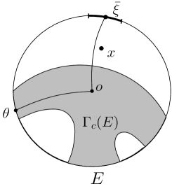
Figure 2. Lemma 6.4

In order to use lemma 6.3, we will show that there exists a constant $\alpha>0$ depending only on $\delta$ and $K$ such that $\{\xi\in\partial S\,|\,(\xi,\bar{\xi})_{x}\geq\alpha\}\subset\partial S\setminus E$.

For $\theta\in E$, we want to bound uniformly from above the product $(\theta,\bar{\xi})_{x}$. Inequality (6.1) gives

$$\min\{(\theta,\bar{\xi})_{x},(o,\theta)_{x}\}\leq(o,\bar{\xi})_{x}+2\delta.$$

By inequality (6.2), $(o,\bar{\xi})_{x}\leq d(x,\bar{\gamma})+2\delta\leq K+2\delta$, so $\min\{(\theta,\bar{\xi})_{x},(o,\theta)_{x}\}\leq K+4\delta$. Again by inequality (6.2), denoting by $\gamma$ a geodesic ray from $o$ to $\theta$, $(o,\theta)_{x}\geq d(x,\gamma)-2\delta\geq c-2\delta>K+4\delta$ and $\min\{(\theta,\bar{\xi})_{x},(o,\theta)_{x}\}=(\theta,\bar{\xi})_{x}\leq K+4\delta$.

Therefore, $\{\xi\in\partial S\,|\,(\xi,\bar{\xi})_{x}\geq K+5\delta\}\cap E=\emptyset$. By lemma 6.3, there exists $\eta>0$ depending only on $\delta$ such that

$$\mathbb{P}_{x}(X_{\infty}\not\in E)\geq\eta.$$

∎

Corollary 6.5.

Let $E$ be a borelian set of $\partial S$, $x\in S$ and $c>c_{1}$. For $\mu$-almost all $\theta\in E$, $\mathbb{P}_{x}^{\theta}$-a.s., the random walk “ends in $\Gamma_{c}(E)$” (Formally, for $\mathbb{P}_{x}^{\theta}$-almost all $\omega$, there exists $N\in\mathbb{N}$ such that for all $n\geq N$, $X_{n}(\omega)\in\Gamma_{c}(E)$).

Proof.

Let $f_{E}(x):=\mathbb{P}_{x}(X_{\infty}\in E)=\mathbb{E}_{x}[\mathbf{1}_{E}(X_{\infty})]$. As a consequence of the representation lemma 5.3 of bounded harmonic functions, for $\mu$-almost all $\theta$, one has

$$\forall x\in S,\,\mathbb{P}_{x}^{\theta}[\lim_{n\to\infty}f_{E}(X_{n})=\mathbf{1}_{E}(\theta)]=1.$$

Because of lemma 6.4, there exists $\eta>0$ such that

$$\forall x\not\in\Gamma_{c}(E),\,f_{E}(x)\leq 1-\eta.$$

Thus for all $x\in S$ and for $\mu$-almost all $\theta\in E$, $\mathbb{P}_{x}^{\theta}$-a.s., $X_{n}$ is in $\Gamma_{c}(E)$ for $n$ large enough. ∎

Given a tube $\Gamma_{c}^{\theta}$ and $R>0$, the set $\Gamma_{c}^{\theta}\setminus B(o,R)$ is called a spike of $\Gamma_{c}^{\theta}$.

Corollary 6.6.

Let $c>c_{1}$ and $E$ be a borelian set of $\partial S$. Then, for all $\theta\in\partial S$ such that ${\displaystyle{\displaystyle\lim_{\stackrel{{\scriptstyle N.T.}}{{x\to\theta}}}}\mathbb{P}_{x}(X_{\infty}\in E)=1}$, $\Gamma_{c}(E)$ contains spikes of every tube with $\theta$ as vertex.

In particular, it is the case for $\mu$-almost all $\theta\in E$ by the bounded harmonic function representation lemma 5.3.

Proof.

Fix $\theta\in\partial S$ such that ${\displaystyle{\displaystyle\lim_{\stackrel{{\scriptstyle N.T.}}{{x\to\theta}}}}\mathbb{P}_{x}(X_{\infty}\in E)={\displaystyle\lim_{\stackrel{{\scriptstyle N.T.}}{{x\to\theta}}}}f_{E}(x)=1}$ and let $\Gamma_{e}^{\theta}$ be a tube with vertex $\theta$. By contradiction, assume that $\Gamma_{c}(E)$ does not contain any spike of this tube. Then, for each $R>0$, there exists $x\in\Gamma_{e}^{\ \theta}\setminus\Gamma_{c}(E)$ such that $d(o,x)>R$.

Let $(x_{k})_{k\in\mathbb{N}}$ be a sequence in $\Gamma_{e}^{\ \theta}\setminus\Gamma_{c}(E)$ such that $d(o,x_{k})>k$. Then $(x_{k})_{k}$ converges to $\theta$ staying in $\Gamma_{e}^{\theta}$ and we have $\lim_{k\to\infty}f_{E}(x_{k})=1.$ Since $x_{k}\not\in\Gamma_{c}(E)$, by lemma 6.4, $f_{E}(x_{k})\leq 1-\eta$, a contradiction. ∎

The following corollary will not intervene later. However, it is remarkable to observe that the behaviour of a harmonic function on a tube $\Gamma_{c_{0}}^{\theta}$ controls the behaviour of this function on every tube $\Gamma_{c}^{\theta}$, $c>0$.

Corollary 6.7.

Given a harmonic function $u$, for all real $c>c_{1}$ one has $\mathcal{N}_{c}\approx\mathcal{N}$.

Proof.

By definition, $\mathcal{N}\subset\mathcal{N}_{c}$. It is thus sufficient to show that $\mathcal{N}_{c}\stackrel{{\scriptstyle\sim}}{{\subset}}\mathcal{N}$ for $c>c_{1}$. Let $c>c_{1}$ and denote by

$$A_{c}^{m}=\{\theta\in\partial S\,|\,N_{c}^{\theta}(u)\leq m\}$$

the set of points $\theta\in\partial S$ such that $u$ is bounded by $m$ on $\Gamma_{c}^{\theta}$. As $\mathcal{N}_{c}$ is the countable union of the $A_{c}^{m}$, we need only to show that $A_{c}^{m}\stackrel{{\scriptstyle\sim}}{{\subset}}\mathcal{N}$ for all $m$. By definition of $A_{c}^{m}$, $|u|$ is bounded by $m$ on $\Gamma_{c}(A_{c}^{m})$. Using corollary 6.6, we obtain that for $\mu$-almost all points $\theta\in A_{c}^{m}$, $\Gamma_{c}(A_{c}^{m})$ contains spikes of all tube with $\theta$ as vertex. On these spikes, the function $u$ is bounded, and therefore, by local finiteness, $u$ is bounded on the tubes, which means that $\theta$ is in $\mathcal{N}$. Finally, $A_{c}^{m}\stackrel{{\scriptstyle\sim}}{{\subset}}\mathcal{N}$ and therefore,

$$\mathcal{N}_{c}\stackrel{{\scriptstyle\sim}}{{\subset}}\mathcal{N}.$$

∎

7. proof of the main result

With geometric lemmas and the stochastic result (proposition 5.2) in hand, we can now prove theorem 4.1.

Proof.

As above, let us denote by

$$A_{c}^{m}=\{\theta\in\partial S\,|\,N_{c}^{\theta}(u)\leq m\}.$$

Since $\mathcal{N}_{c}$ is a countable union of the sets $A_{c}^{m}$, it is sufficient to prove that for all $m$ and all $c>c_{1}+m_{1}$, $A_{c}^{m}\stackrel{{\scriptstyle\sim}}{{\subset}}\mathcal{L}_{c-m_{1}}$. Then, we will have $\mathcal{N}_{c}\stackrel{{\scriptstyle\sim}}{{\subset}}\mathcal{L}_{c-m_{1}}$ and since for $c>c^{\prime}$, $\mathcal{L}_{c}\subset\mathcal{L}_{c^{\prime}}$, we can conclude that $\mathcal{N}\stackrel{{\scriptstyle\sim}}{{\subset}}\mathcal{L}$.

Let $c>c_{1}+m_{1}$. We shall first prove that $A_{c}^{m}\stackrel{{\scriptstyle\sim}}{{\subset}}\mathcal{L}^{*}$. Applying corollary 6.5 to the borelian set $A_{c}^{m}$, we get: for $\mu$-almost all point $\theta\in A_{c}^{m}$, $\mathbb{P}_{z}^{\theta}$-almost surely, $(X_{k})_{k\geq 0}$ ends in $\Gamma:=\Gamma_{c-m_{1}}(A_{c}^{m})$. Let $\theta$ be such a point. The key point is that for all $x\in\Gamma$ and all $y\in S$ such that $d(x,y)\leq m_{1}$, $|u(y)|\leq m$. It implies in particular that for $\mathbb{P}_{z}^{\theta}$-almost all $\omega$, there exists $N\in\mathbb{N}$ such that for all $n\geq N$ and all $y\in S$ such that $d(y,X_{n}(\omega))\leq m_{1}$, we have $|u(y)|\leq m$. By local finiteness, $\mathbb{P}_{z}^{\theta}$-almost surely, $\widetilde{N^{*}}<+\infty$. Thus, $\mathbb{P}_{z}^{\theta}(\widetilde{\mathcal{N}^{**}})=1$, $\theta\in\widetilde{\mathcal{N}^{*}}$ and hence $A_{c}^{m}\stackrel{{\scriptstyle\sim}}{{\subset}}\widetilde{\mathcal{N}^{*}}$. However, by proposition 5.2, $\widetilde{\mathcal{N}^{*}}\stackrel{{\scriptstyle\sim}}{{\subset}}\mathcal{L}^{*}$, so

$$A_{c}^{m}\stackrel{{\scriptstyle\sim}}{{\subset}}\mathcal{L}^{*}.$$

Let us now prove that $A_{c}^{m}\stackrel{{\scriptstyle\sim}}{{\subset}}\mathcal{L}_{c-m_{1}}$. As shown above, for $\mu$-almost all $\theta\in A_{c}^{m}$, $\mathbb{P}_{z}^{\theta}$-almost surely, $(u(X_{n}))_{n}$ has a finite limit $\ell(\theta)$. It defines a function $\ell$ on $A_{c}^{m}$. We use again corollary 6.5: for $\mu$-almost all $\theta\in A_{c}^{m}$, $\mathbb{P}_{z}^{\theta}$-almost surely, $X_{n}$ is in $\Gamma$ for $n$ big enough. This together with the fact that $|u|$ is bounded by $m$ on $\Gamma$ implies that $|\ell|\leq m$ on $A_{c}^{m}$.

We will conclude this proof using a method of J. Brossard [Bro78]. We will decompose $u$ on $\Gamma$ as a sum of three functions which will have non-tangential limits at almost all points of $A_{c}^{m}$.

We define the function

$$f(z):=\mathbb{E}_{z}\left[(\ell\cdot\mathbf{1}_{A_{c}^{m}})(X_{\infty})\right].$$

By the representation lemma 5.3, $f$ is a bounded harmonic function which converges non-tangentially at $\mu$-almost all point $\theta\in\partial S$ to $(\ell\cdot\mathbf{1}_{A_{c}^{m}})(\theta)$. Denote by $\tau$ the exit time of the set $\Gamma$ and $\tau_{k}$ the exit time of $B(o,k)$. Since $u$ is bounded and harmonic on the thickened set $\widetilde{\Gamma}\cap\widetilde{B(o,k)}=\{y\in S\,|\,d(y,\Gamma\cap B(o,k))\leq m_{1}\}$, which is a bounded set, ${u(z)=\mathbb{E}_{z}[u(X_{\tau\wedge\tau_{k}})]}$. If $\tau=+\infty$, $\mathbb{P}_{z}$-almost surely, $(X_{n})_{n}$ converges to a point $X_{\infty}\in A_{c}^{m}$, so $\mathbb{P}_{z}$-almost surely, $(u(X_{n}))_{n}$ goes to $\ell(X_{\infty})$. We can extend $u$ to $A_{c}^{m}$ by setting $u(\theta):=\ell(\theta)$ for $\theta\in A_{c}^{m}$. Since $|u|$ is bounded by $m$ on $\Gamma$, we can apply Lebesgue’s theorem to obtain

$$\forall z\in\Gamma,u(z)=\mathbb{E}_{z}[u(X_{\tau})].$$

Decomposing the event $\{X_{\infty}\in A_{c}^{m}\}$ into the union ${\{\tau<\infty;X_{\infty}\in A_{c}^{m}\}\cup\{\tau=\infty\}}$ we obtain, for $z\in\Gamma$,

$$u(z) =\mathbb{E}_{z}[u(X_{\tau})\cdot\mathbf{1}_{\{\tau<\infty\}}]+\mathbb{E}_{z}[u(X_{\infty})\cdot\mathbf{1}_{\{\tau=\infty\}}]$$

$$=\mathbb{E}_{z}[u(X_{\tau})\cdot\mathbf{1}_{\{\tau<\infty\}}]+\mathbb{E}_{z}[u(X_{\infty})\cdot\mathbf{1}_{\{X_{\infty}\in A_{c}^{m}\}}]$$

$$-\mathbb{E}_{z}[u(X_{\infty})\cdot\mathbf{1}_{\{X_{\infty}\in A_{c}^{m}\}}\cdot\mathbf{1}_{\{\tau<\infty\}}].$$

This is exactly the announced decomposition. Indeed, denoting $g(z)=\mathbb{E}_{z}[u(X_{\tau})\cdot\mathbf{1}_{\{\tau<\infty\}}]$ and $h(z)=-\mathbb{E}_{z}[u(X_{\infty})\cdot\mathbf{1}_{\{X_{\infty}\in A_{c}^{m}\}}.\mathbf{1}_{\{\tau<\infty\}}]$, we have $u=f+g+h$ on $\Gamma$.

It remains to prove that at almost all point $\theta$ in $A_{c}^{m}$, the functions $g(z)$ and $h(z)$ converge to zero when $z$ goes to $\theta$ staying in the tube $\Gamma_{c-m_{1}}^{\theta}$. Since $u$ is bounded on $\widetilde{\Gamma}=\{y\in S\,|\,d(y,\Gamma)\leq m_{1}\}$, if $\tau<\infty$, then $|u(X_{\tau})|\leq m$ and obviously

$$|g(z)|\leq m\cdot\mathbb{P}_{z}(\tau<\infty).$$

In the same way, for almost all $\theta\in A_{c}^{m}$, $|u(\theta)|\leq m$, so we obtain easily by conditioning

$$|h(z)|\leq m\cdot\mathbb{P}_{z}(\tau<\infty).$$

It is now sufficient to prove that for almost all $\theta\in A_{c}^{m}$, $\mathbb{P}_{z}(\tau<\infty)$ goes to zero when $z$ goes to $\theta$ staying in $\Gamma_{c-m_{1}}^{\theta}$. This follows from lemma 6.4. Indeed, there exists $\eta>0$ such that

$$\forall z\not\in\Gamma,\mathbb{P}_{z}(X_{\infty}\not\in A_{c}^{m})\geq\eta$$

and in particular this holds for all $z\in\widetilde{\Gamma}\setminus\Gamma$. The strong Markov property implies that for all $z\in\Gamma$,

$$\mathbb{P}_{z}(X_{\infty}\not\in A_{c}^{m}) =\mathbb{P}_{z}(\{X_{\infty}\not\in A_{c}^{m}\}\cap\{\tau<\infty\})$$

$$=\sum_{i=1}^{\infty}\mathbb{P}_{z}(\{X_{\infty}\not\in A_{c}^{m}\}\cap\{\tau=i\})$$

$$=\sum_{i=1}^{\infty}\mathbb{E}_{z}\left[\mathbb{E}_{z}\left[\mathbf{1}_{\{X_{\infty}\not\in A_{c}^{m}\}}\cdot\mathbf{1}_{\{\tau=i\}}|\mathcal{F}_{i}\right]\right]$$

$$=\sum_{i=1}^{\infty}\mathbb{E}_{z}\left[\mathbb{E}_{z}\left[\mathbf{1}_{\{X_{\infty}\not\in A_{c}^{m}\}}|\mathcal{F}_{i}\right]\cdot\mathbf{1}_{\{\tau=i\}}\right]$$

$$=\sum_{i=1}^{\infty}\mathbb{E}_{z}[\mathbb{P}_{X_{i}}(X_{\infty}\not\in A_{c}^{m})\cdot\mathbf{1}_{\{\tau=i\}}]$$

$$=\mathbb{E}_{z}[\mathbb{P}_{X_{\tau}}(X_{\infty}\not\in A_{c}^{m})\cdot\mathbf{1}_{\{\tau<\infty\}}]$$

$$\geq\eta\cdot\mathbb{P}_{z}(\tau<\infty).$$

By lemma 5.3, for almost all $\theta\in A_{c}^{m}$, ${\displaystyle\lim_{\stackrel{{\scriptstyle N.T.}}{{z\to\theta}}}}\mathbb{P}_{z}(X_{\infty}\not\in A_{c}^{m})=0$. It follows that for almost all $\theta\in A_{c}^{m}$, $\mathbb{P}_{z}(\tau<\infty)$ goes to zero when $z$ goes to $\theta$ staying in $\Gamma_{c-m_{1}}^{\theta}$.
We thus have that $A_{c}^{m}\stackrel{{\scriptstyle\sim}}{{\subset}}\mathcal{L}_{c-m_{1}}$ and the theorem is proved.

∎

References

- [Anc87] Ancona, A., Negatively curved manifolds, elliptic operators, and the Martin boundary, Ann. of Math. (2) 125 (1987), no. 3, 495-536.
- [Anc88] Ancona, A., Positive harmonic functions and hyperbolicity. Potential theory, surveys and problems (Prague, 1987), 1-23, Lecture Notes in Math., 1344, Springer, Berlin, 1988.
- [Anc90] Ancona, A., Théorie du potentiel sur les graphes et les variétés, École d’été de Probabilités de Saint-Flour XVIII-1988, 1-112, Lecture Notes in Math., 1427, Springer, Berlin, 1990.
- [AnS85] Anderson, M.T., Schoen, R., Positive harmonic functions on complete manifolds of negative curvature, Ann. of Math. (2) 121 (1985), no. 3, 429-461.
- [Bri99] Bridson, M.R., Haefliger, A., Metric spaces of non-positive curvature, Grundlehren der Mathematischen Wissenschaften, 319. Springer-Verlag, Berlin, 1999.
- [Bro78] Brossard, J., Comportement non-tangentiel et comportement brownien des fonctions harmoniques dans un demi-espace. Démonstration probabiliste d’un théorème de Calderon et Stein, Séminaire de Probabilités, XII (Univ. Strasbourg, Strasbourg, 1976/1977), pp. 378-397, Lecture Notes in Math., 649, Springer, Berlin, 1978.
- [Cal50a] Calderón, A.P. On a theorem of Marcinkiewicz and Zygmund, Trans. Amer. Math. Soc. 68, (1950). 55-61.
- [Cal50b] Calderón, A.P. On the behaviour of harmonic functions at the boundary, Trans. Amer. Math. Soc. 68, (1950). 47-54.
- [Car72] Cartier, P., Fonctions harmoniques sur un arbre, Symposia Mathematica, Vol. IX (Convegno di Calcolo delle Probabilità, INDAM, Rome, 1971), 203-270. Academic Press, London, 1972.
- [Der75] Derriennic, Y., Marche aléatoire sur le groupe libre et frontière de Martin, Z. Wahrscheinlichkeitstheorie und Verw. Gebiete 32 (1975), no. 4, 261-276.
- [Doo57] Doob, J.L., Conditional Brownian motion and the boundary limits of harmonic functions, Bull. Soc. Math. France 85 1957 431-458.
- [Dur84] Durrett, R., Brownian motion and martingales in analysis, Wadsworth Mathematics Series. Wadsworth International Group, Belmont, CA, 1984.
- [Dyn69] Dynkin, E.B., The boundary theory of Markov processes (discrete case). (Russian) Uspehi Mat. Nauk 24 1969 no. 2 (146), 3-42.
- [Fat06] Fatou, P., Séries trigonométriques et séries de Taylor, Acta Math. 30 (1906), no. 1, 335-400.
- [GdlH90] Ghys, E., de la Harpe, P., Espaces métriques hyperboliques. Sur les groupes hyperboliques d’après Mikhael Gromov (Bern, 1988), Progr. Math., 83, Birkhauser Boston, Boston, MA, 1990.
- [Gro81] Gromov, M., Hyperbolic manifolds, groups and actions. Riemannian surfaces and related topics, 183-213, Ann. of Math. Stud., 97, Princeton Univ. Press, Princeton, N.J., 1981.
- [Mou94] Mouton, F., Convergence Non-Tangentielle des Fonctions Harmoniques en Courbure Négatives, thèse de troisième cycle, Grenoble, 1994.
- [Mou00] Mouton, F., Comportement asymptotique des fonctions harmoniques sur les arbres, Séminaire de Probabilités, XXXIV, 353-373, Lecture Notes in Math., 1729, Springer, Berlin, 2000.
- [Ste61] Stein, E.M., On the theory of harmonic functions of several variables. II. Behavior near the boundary, Acta Math. 106 1961 137-174.
- [Woe00] Woess, W., Random walks on infinite graphs and groups, Cambridge Tracts in Mathematics, 138. Cambridge University Press, Cambridge, 2000.