Galactic chemical evolution in hierarchical formation models - I. Early-type galaxies in the local Universe

Abstract

We study the metallicities and abundance ratios of early-type galaxies in cosmological semi-analytic models (SAMs) within the hierarchical galaxy formation paradigm. To achieve this we implemented a detailed galactic chemical evolution (GCE) model and can now predict abundances of individual elements for the galaxies in the semi-analytic simulations. This is the first time a SAM with feedback from Active Galactic Nuclei (AGN) has included a chemical evolution prescription that relaxes the instantaneous recycling approximation. We find that the new models are able to reproduce the observed mass-metallicity ($M_{\star}$–[Z/H]) relation and, for the first time in a SAM, we reproduce the observed positive slope of the mass-abundance ratio ($M_{\star}$–[$\alpha$/Fe]) relation. Our results indicate that in order to simultaneously match these observations of early-type galaxies, the use of both a very mildly top-heavy IMF (i.e., with a slope of $x=1.15$ as opposed to a standard $x=1.3$), and a lower fraction of binaries that explode as Type Ia supernovae appears to be required. We also examine the rate of supernova explosions in the simulated galaxies. In early-type (non-star forming) galaxies, our predictions are also consistent with the observed SNe rates. However, in star-forming galaxies, a higher fraction of SN Ia binaries than in our preferred model is required to match the data. If, however, we deviate from the classical model and introduce a population of SNe Ia with very short delay times, our models simultaneously produce a good match to the observed metallicities, abundance ratios and SN rates.

1 Introduction

The chemical properties and abundance ratios of galaxies provide important constraints on their formation histories. Galactic chemical evolution has been modelled in detail in the monolithic collapse scenario (e.g., Matteucci & Greggio, 1986; François et al., 2004; Romano et al., 2005; Pipino & Matteucci, 2004, 2006). These models have successfully described the abundance distributions in our Galaxy and other spiral discs, as well as the trends of metallicity and abundance ratios observed in early-type galaxies. In the last three decades, however, the paradigm of hierarchical assembly in a Cold Dark Matter (CDM) cosmology has revised the picture of how structure in the Universe forms and evolves. In this scenario, galaxies form when gas radiatively cools and condenses inside dark matter haloes, which themselves follow dissipationless gravitational collapse (White & Rees, 1978; White & Frenk, 1991). The CDM picture has been successful at predicting many observed properties of galaxies, though many potential problems and open questions remain. It is therefore interesting to see whether chemical evolution models, when implemented within this modern cosmological context, are able to correctly predict the observed chemical properties of galaxies.

The semi-analytic approach provides a cosmological framework in which to study galaxy formation and chemical evolution in different environments, by following the merger history of dark matter haloes and the relevant physical processes such as gas cooling, star formation and feedback (e.g. White & Frenk, 1991; Kauffmann et al., 1993; Cole et al., 1994; Cole et al., 2000; Hatton et al., 2003; Somerville & Primack, 1999; Somerville et al., 2001). A major challenge for models of galaxy formation within the CDM picture arises from the mismatch between the shape of the mass function of the dark matter haloes and that of the baryonic condensations that we call galaxies (White & Frenk, 1991; Kauffmann et al., 1993; Somerville & Primack, 1999; Benson et al., 2003). The CDM theory predicts a steeper slope for low-mass halos, and a more gradual drop-off in the abundance of high-mass halos than is seen in luminous galaxies, implying that the formation of stars must be inefficient in both low-mass and high-mass haloes (Moster et al., 2009). However, the inclusion of physically motivated, if still ad hoc, feedback processes in the semi-analytic models can cure these discrepancies. The faint end of the luminosity function can be matched with a combination of supernova feedback and suppression of gas cooling in low mass haloes as a result of a photo-ionising background. At the bright end, heating by giant radio jets powered by accreting black holes has become a favored mechanism for preventing over-cooling and quenching star formation in massive halos (Croton et al., 2006; Bower et al., 2006; Somerville et al., 2008). This latest generation of semi-analytic models (‘SAMs’) is successful at reproducing many properties of galaxies at the present and at high redshift, for example, the luminosity and stellar mass function of galaxies, color-magnitude or star formation rate vs. stellar mass distributions, relative numbers of early and late-type galaxies, gas fractions and size distributions of spiral galaxies, and the global star formation history (e.g. Croton et al., 2006; Bower et al., 2006; Cattaneo et al., 2006; De Lucia et al., 2006; Somerville et al., 2008; Kimm et al., 2009; Fontanot et al., 2009, to name just a few).

The modelling of chemical enrichment of the galaxies and intergalactic (and intracluster) gas, however, has not been thoroughly developed in semi-analytic models, and to date most SAMs have only used the instantaneous recycling approximation (in essence only considering enrichment by type II supernovae) and trace only the total metal content. There are, however, a few models that have included a more refined treatment of the chemical enrichment. Thomas (1999) and Thomas & Kauffmann (1999) were the first to include enrichment by type Ia supernovae (SNe Ia) in models with cosmologically motivated star formation histories. However, rather than implementing the chemical evolution self-consistently within a semi-analytic model, they made use of star formation histories from the SAM and assumed a closed-box model (no gas inflows or outflows) for the chemical evolution. They calculated the evolution of [Fe/H] and [Mg/Fe] and found a decreasing trend of [Mg/Fe] with increasing galaxy luminosity, in stark disagreement with observations (e.g. Worthey et al., 1992; Trager et al., 2000a, b; Thomas et al., 2005).

The first semi-analytic model to self-consistently track a variety of elements due to enrichment by SNe Ia and type II supernovae (SNe II) was that of Nagashima et al. (2005a, b). Among other things, they adopted a bimodal IMF described by a standard IMF for normal quiescent star formation in discs and an extremely flat ‘top-heavy’ IMF during merger-driven starbursts. This model was motivated by the difficulty that semi-analytic models with a standard IMF experienced in reproducing the observed population of very luminous sub-mm galaxies at high redshift (Baugh et al., 2005). However, the notion that early-type galaxies form their stars with an IMF flatter than standard is not new and has been proposed many times in the past as a plausible explanation for the abundance patterns in early-type galaxies and in the ICM of galaxy clusters (e.g., Worthey, Faber & Gonzalez, 1992; Matteucci & Gibson, 1995; Gibson & Matteucci, 1997; Thomas, Greggio & Bender, 1999). The predictions of the Nagashima et al. model were in good agreement with the abundances of the intracluster medium (ICM) of galaxy clusters, matching the trend of individual elements (O, Fe, Mg, Si) and abundance ratios with ICM temperature. However, the same model failed to reproduce the trend of [$\alpha$/Fe] in early-type galaxies, where they found that the abundance ratio decreases with increasing galactic velocity dispersion, again in clear contradiction with observations. Very recently, Pipino et al. (2008) have coupled galactic chemical evolution to the GalICS semi-analytic model (Hatton et al., 2003), and obtained results similar to those of Nagashima et al. (2005b).

In a simple closed-box picture, it is well-known that galaxies with short star formation timescales are expected to have enhanced [$\alpha$/Fe] ratios (because their enrichment is dominated by $\alpha$-rich Type II SNe), while galaxies with extended star formation histories tend to have lower [$\alpha$/Fe] (e.g. Worthey et al., 1992; Thomas et al., 1999; Thomas, 1999; Thomas & Kauffmann, 1999; Trager et al., 2000b), because of the additional Fe contributed by delayed Type Ia enrichment. Therefore a possible interpretation of the difficulties that CDM-based galaxy formation models have experienced in reproducing the positive trend between mass, luminosity, or velocity dispersion and abundance ratio is related to the issue of so-called “downsizing”. This refers to the variety of observational evidence that high-mass galaxies formed their stars early and over short timescales, while low-mass galaxies have more extended star formation histories (see Fontanot et al., 2009, for a summary). Before the inclusion of AGN feedback or some other mechanism that quenches star formation in massive halos, CDM-based galaxy formation models predicted the opposite trend (massive galaxies continued to accrete gas and form stars until the present day, leading to extended star formation histories). It has been demonstrated that including radio-mode AGN feedback in semi-analytic models leads to a “downsizing” trend for star formation that is at least qualitatively in better agreement with observations (De Lucia et al., 2006; Somerville et al., 2008; Trager & Somerville, 2009; Fontanot et al., 2009). Therefore we expect that the new models might do better at reproducing the trend of [$\alpha$/Fe] with mass as the more massive galaxies will have shorter star formation timescales.

Clearly, observations of chemical abundances and abundance ratios in various phases (stellar, ISM, ICM) offer the opportunity to obtain strong constraints on galaxy formation histories and the physics that shapes them. However, in order to take advantage of these observations, it is necessary to implement detailed modeling of chemical evolution into a full modern SAM that includes the relevant physical processes (e.g. triggered star formation and morphological transformation of galaxies via mergers, the growth of supermassive black holes, and AGN feedback). In this work we incorporate detailed chemical evolution into the semi-analytic galaxy formation model of Somerville et al. (2008), taking into account enrichment by SNe Ia, SNe II and long-lived stars, and abandoning the instantaneous recycling approximation by considering the finite lifetimes of stars of all masses. The delay in the metal enrichment by SNe Ia is calculated self-consistently according to the lifetimes of the progenitor stars. This is, to our knowledge, the first time that detailed chemical evolution has been included in a semi-analytic model with AGN feedback (both radio-mode heating and AGN-driven winds). The base model includes gas inflows due to radiative cooling of gas and outflows due to supernova and AGN-driven winds. We compute the abundances of many $\alpha$ and Fe-peak elements for early-type galaxies of different masses, exploring different IMF slopes and values for the fraction of binaries that yield a SN Ia event, and compare these with observations of abundances and abundance ratios for a sample of local early-type galaxies. We also calculate SNe rates using both the classical Greggio & Renzini (1983) approach for type Ia SN and the more recent Delay-Time-Distribution (DTD) formalism (Greggio, 2005). Another improvement in the present work is our use of re-calibrated estimates for chemical abundances obtained from line-strengths in early type galaxies (see Appendix B for details).

The outline of the paper is as follows. In Section 2 we give an overview of the main ingredients of the semi-analytic model. In Section 3 we describe in detail the adopted treatment for the chemical evolution. In Section 4 we present our predictions and compare them with observations. In Section 5 we summarise our findings and present our conclusions. Two appendices describe the detailed implementation of the chemical evolution model and the data used in this paper.

2 The semi-analytic model

In this section we summarise the basic ingredients of the SAM used to model the formation and evolution of galaxies. These include the growth of structure of the dark matter component in a hierarchical clustering framework, radiative cooling of gas, star formation, supernova feedback, AGN feedback, galaxy merging within dark matter haloes, metal enrichment of the ISM and ICM, and the evolution of stellar populations. The reader is referred to Somerville & Primack (1999), Somerville et al. (2001) and especially Somerville et al. (2008, hereafter S08) for a comprehensive and detailed description of the different prescriptions used in this semi-analytic model. In what follows we briefly sketch the modelling of the most important physical processes.

2.1 Dark matter merger trees and galaxy merging

The merging histories (or merger trees) of dark matter haloes are constructed based on the Extended Press-Schechter formalism using the method described in Somerville & Kolatt (1999), with improvements described in S08. Each branch in the tree represents a merger event, and, in order to make the process finite, the trees are followed down to a minimum progenitor mass of $10^{10}\,M_{\sun}$.

Whenever dark matter haloes merge, the central galaxy of the largest progenitor becomes the new central galaxy, and all others become ‘satellites’. Satellite galaxies may eventually merge with the central galaxy due to dynamical friction. To model the timescale of the merger process we use a variant of the Chandrasekhar formula from Boylan-Kolchin et al. (2008). Tidal stripping and destruction of satellites are also included as described in S08.

2.2 Gas cooling, star formation and supernova feedback

Before the Universe is reionised, each halo contains a mass of hot gas equal to the universal baryon fraction times the virial mass of the halo. After reionisation, the photo-ionising background can suppress the collapse of gas into low-mass halos. We use the results of Gnedin (2000) and Kravtsov et al. (2004) to model the fraction of baryons that can collapse into haloes of a given mass after reionisation.

When a dark matter halo collapses, or merges with a larger halo, the gas within it is shock-heated to the virial temperature of the halo, and gradually radiates and cools at a rate given by the cooling function. To calculate this function we use the metallicity-dependent radiative cooling curves of Sutherland & Dopita (1993). A detailed description of how the cooling process is modelled can be found in S08. The rate at which gas can cool is given by:

$$\dot{m}_{\mathrm{cool}}=\frac{1}{2}m_{\mathrm{hot}}\frac{r_{\mathrm{cool}}}{r_{\mathrm{vir}}}\frac{1}{t_{\mathrm{cool}}},$$ (1)

where $m_{\mathrm{hot}}$ is the mass of the hot halo gas, $r_{\mathrm{vir}}$ is the virial radius of the dark matter halo, $r_{\mathrm{cool}}$ is the radius within which all of the gas can cool in a time $t_{\mathrm{cool}}$, which itself depends on density, metallicity and temperature. In our models, we assume that the cold gas is accreted only by the central galaxy of the halo, but in reality satellite galaxies should also receive some measure of new cold gas. This aspect of the modelling should be improved (cf. Pipino et al., 2008) and for the present study we restrict our analysis to only the central galaxy of each halo, except when otherwise stated.

When the gas cools we assume that it settles into a rotationally supported disc. The radial sizes of the discs are calculated according to the results described in Somerville et al. (2008), and agree well with observed disc sizes to $z\sim 2$.

We model the star formation rate in quiescent discs with a recipe based on the empirical Schmidt-Kennicutt law (Kennicutt, 1989):

$$\dot{m}_{\star} = \frac{2\pi A_{K}\Sigma_{0}^{N_{K}}r_{\mathrm{gas}}^{2}}{N_{K}^{2}}$$ (2)

$$\times\left[1-\left(1+\frac{N_{K}r_{\mathrm{crit}}}{r_{\mathrm{gas}}}\right)\exp(-N_{K}r_{\mathrm{crit}}/r_{\mathrm{gas}})\right]$$

where $\dot{m}_{\star}$ is the star formation rate, $\Sigma_{0}\equiv m_{\mathrm{cold}}/(2\pi r_{\mathrm{gas}}^{2})$ is the average surface density of the cold gas, $r_{\mathrm{gas}}$ is the scale-length of the gaseous disc (assumed to be an exponential disc with its scale-length proportional to that of the stellar disc), $r_{\mathrm{crit}}$ is the radius at which the gas reaches the critical surface density threshold for star formation ($\Sigma_{\mathrm{crit}}$), and $A_{K}$ and $N_{K}$ are the normalisation and slope of the SFR law. We adopt the values $A_{K}=8.35\times 10^{-5}$, $N_{K}=1.4$ and $\Sigma_{\mathrm{crit}}=6\,M_{\sun}{\mathrm{pc}^{-2}}$, as in S08.

Galaxy mergers in the SAM trigger enhanced episodes of star formation. The burst is modelled by two parameters, the time-scale and the efficiency of the burst. The time-scale is a function of the virial velocity of the progenitor galaxies, the equation of state of the gas, the cold gas fraction in the discs, and the redshift (Robertson et al., 2006). The efficiency, which is defined as the fraction of the cold gas reservoir (of both galaxies) that is turned into stars during the burst, is assumed to be a power-law function of the mass ratio of the merging galaxies, and the exponent of the power-law depends on the galaxy morphology (Cox et al., 2008). The collisional starburst occurs in addition to any ongoing ‘normal’ quiescent star formation, which continues uninterrupted through the merger but is usually insignificant in comparison to the burst. Any new stars formed during the burst are always placed in the bulge component of the resulting galaxy.

As supernovae occur, they inject energy into the ISM and reheat the cold gas, which is then expelled from the disc and incorporated into the hot halo gas where it can cool again. The rate of reheating by SNe is given by

$$\dot{m}_{\mathrm{rh}}=\epsilon_{0}^{SN}\left(\frac{V_{\mathrm{disc}}}{200\,\mathrm{km/s}}\right)^{-\alpha_{\mathrm{rh}}}\dot{m}_{\star},$$ (3)

where $\epsilon_{0}^{SN}$ and $\alpha_{\mathrm{rh}}$ are free parameters. The circular velocity of the disc $V_{\mathrm{disc}}$ is taken to be equal to the maximum rotational velocity of the dark matter halo. Some fraction of the reheated gas can also be ejected from the halo entirely into the diffuse Intergalactic Medium. This fraction is described by:

$$f_{\mathrm{eject}}(V_{\mathrm{vir}})=[1.0+(V_{\mathrm{vir}}/V_{\mathrm{eject}})^{\alpha_{\mathrm{eject}}}]^{-1},$$ (4)

where $\alpha_{\mathrm{eject}}=6$ and $V_{\mathrm{eject}}$ is a free parameter in the range $\simeq 100-150$ km/s. This ejected gas is allowed to re-collapse into the halo at later times and once again becomes available for cooling.

2.3 Formation of Spheroids

In most semi-analytic models each merger is classified as ‘major’ or ‘minor’ depending on whether the ratio of the smaller to the larger galaxies’ baryonic masses is greater than or less than the parameter $f_{\mathrm{ellip}}\sim 0.25$, respectively. The usual assumption is then that, in a major merger, the bulge and disc stars of both progenitor galaxies, as well as the stars formed in the merger driven starburst (see below), are transferred to the bulge component of the resulting galaxy. In a minor merger, all the pre-existing stars of the smaller galaxy end up in the disc of the post-merger galaxy, and all the newly formed stars are placed in bulge. We follow a similar practise here, but instead of using a sharp threshold to define major or minor mergers, we use a more gradual transition function. In detail, when two galaxies with bulge masses $B_{1}$ and $B_{2}$, and disc masses $D_{1}$ and $D_{2}$ merge, the resulting galaxy has a bulge mass $B_{\mathrm{new}}=B_{1}+B_{2}+f_{\mathrm{sph}}(D_{1}+D_{2})$ and a disc mass $D_{\mathrm{new}}=(1-f_{\mathrm{sph}})(D_{1}+D_{2})$. The value $f_{\mathrm{sph}}$ is a continuous function of the total mass ratio (baryons and dark matter) in the central parts of the galaxy (see S08).

2.4 Black Hole Growth and AGN Feedback

The models of S08 also track the growth of super-massive black holes and the energy they release. Each top-level DM halo is seeded with a $\sim 100$ ${\rm M}_{\odot}$ black hole, and these black holes are able to grow via two different accretion modes. The first accretion mode is fuelled by cold gas that is driven into the nucleus of the galaxy by mergers. This mode is radiatively efficient, and the accretion rates are close to the Eddington limit. Because this accretion mode is associated with optically bright classical quasars and AGN, it is referred to as ‘bright mode’ or ‘quasar mode’ accretion. The second mode is fuelled by hot gas in a quasi-hydrostatic halo, and the accretion rate is modelled via the Bondi-Hoyle approximation. Accretion rates in this mode are significantly sub-Eddington ($\sim 10^{-4}$ to $10^{-3}$ times the Eddington rate) and the accretion is assumed to be radiatively inefficient. This mode is, however, associated with the production of giant radio jets, and is therefore referred to as the ‘radio mode’.

Energy released during ‘bright mode’ activity can couple with the cold gas in the galaxy via radiation pressure, driving galactic scale winds that can eject cold gas from the galaxy. The mass outflow rate due to the AGN driven wind is modelled by the following formula:

$$\dot{m}_{\mathrm{agn}}=\epsilon_{\mathrm{wind}}\eta_{\mathrm{rad}}\frac{c}{V_{\mathrm{esc}}}\dot{m}_{\mathrm{acc}},$$ (5)

where $\epsilon_{\mathrm{wind}}$ is the effective coupling efficiency, $V_{\mathrm{esc}}$ is the escape velocity of the galaxy and $\dot{m}_{\mathrm{acc}}$ is the accretion rate of mass onto the black hole.

The radio jets produced by ‘radio mode’ activity are assumed to inject thermal energy into the hot halo gas, partly or completely offsetting the cooling flow. This process is responsible for quenching the star formation in massive galaxies (which contain massive black holes) and solves the ‘over-cooling problem’ that plagued CDM-based galaxy formation models for many years.

2.5 Stellar Population Synthesis and Dust

In order to compare the luminosities and colours of the galaxies in the simulations with real observations, we convolve the star formation and chemical enrichment history of each galaxy with the multi-metallicity simple stellar population (SSP) models of Bruzual & Charlot (2003). We use the models based on the Padova1994 (Bertelli et al., 1994) isochrones with a Chabrier (2001) IMF.

We also model the effects of dust extinction. Based on the model of Charlot & Fall (2000), we consider extinction due to two components, one due to the diffuse dust in the disc and another associated with the dense ‘birth clouds’ surrounding young star forming regions. The $V$-band, face-on extinction optical depth of the diffuse dust is given by

$$\tau_{V,0}\propto\tau_{\mathrm{dust,0}}Z_{\mathrm{cold}}m_{\mathrm{cold}}/(r_{\mathrm{gas}})^{2},$$ (6)

where $\tau_{\mathrm{dust,0}}$ is a free parameter, $Z_{\mathrm{cold}}$ is the metallicity of the cold gas, $m_{\mathrm{cold}}$ is the mass of the cold gas in the disc, and $r_{\mathrm{gas}}$ is the radius of the cold gas disc. To compute the actual extinction we assign each galaxy a random inclination and use a standard ‘slab’ model. Additionally, stars younger than $10^{7}$ yr are enshrouded in a cloud of dust with optical depth $\tau_{\mathrm{BC,V}}=\mu_{\mathrm{BC}}\tau_{V,0}$, where $\mu_{\mathrm{BC}}=3$. Finally, to extend the extinction correction to other wavebands, we assume a Galactic attenuation curve (Cardelli et al., 1989) for the diffuse dust component and a power-law extinction curve $A_{\lambda}\propto(\lambda/5500\AA)^{n}$, with $n=0.7$, for the birth clouds.

2.6 Cosmological and Galaxy Formation Parameters

We adopt a flat $\Lambda$CDM cosmology with $\Omega_{0}=0.2383,\ \Omega_{\Lambda}=0.7617,\ h\equiv H_{0}/(100\,\mathrm{km\ s}^{-1}\mathrm{Mpc}^{-1})=0.732,\ \sigma_{8}=0.761$, and a cosmic baryon fraction of $f_{b}=0.1746$, following the results of Spergel et al. (2007). We adopt these parameters for consistency with the published models of S08, but find that we obtain nearly identical results with the updated values of the cosmological parameters from Komatsu et al. (2009).

We leave the values of the free parameters associated with the galaxy formation models fixed to the fiducial values given in S08. These values were chosen by requiring that the models reproduced key observations of nearby galaxies, such as the $z\sim 0$ stellar mass function, and gas fractions and star formation rates as a function of stellar mass. These models have also been shown to produce reasonable agreement with observed local galaxy colour distributions in Kimm et al. (2009), and with observed stellar mass functions and star formation rates at high redshift ($0<z<4$; Fontanot et al., 2009). In § 4.1 we check that our new models, with the updated treatment of chemical evolution modelling, still reproduce the key observational quantities with the same values of the free parameters.

3 Galactic Chemical Evolution

In S08, the production of metals was tracked using a simple approach commonly adopted in semi-analytic models (see e.g. Somerville & Primack, 1999; Cole et al., 2000; De Lucia et al., 2004; , Kang et al.2005). In a given time-step, when we create a parcel of new stars ${\rm d}m_{*}$, we also create a mass of metals ${\rm d}M_{Z}=y\,{\rm d}m_{*}$, which we assume to be instantaneously mixed with the cold gas in the disc. The yield $y$ is assumed to be constant, and is treated as a free parameter. We track the mean metallicity of the cold gas $Z_{\rm cold}$, and when we create a new parcel of stars they are assumed to have the same metallicity as the mean metallicity of the cold gas in that time-step. Supernova feedback ejects metals from the disc, along with cold gas. These metals are either mixed with the hot gas in the halo, or ejected from the halo into the ‘diffuse’ Intergalactic Medium (IGM), in the same proportion as the reheated cold gas. The ejected metals in the ‘diffuse gas’ reservoir are also re-accreted into the halo in the same manner as the gas.

In the present study, we discard the instantaneous recycling approximation and allow the ISM to be enriched by the products of type Ia and type II supernovae on their own timescales. Consequently, we now track individual elements, and not just the total metal content. The integrated ejecta of each element is not a free parameter, but instead is calculated according to theoretical yields and the star-formation histories provided by the SAM. In the next subsection we describe the implementation of the new chemical evolution model in detail.

3.1 Basic equations of the GCE

For the purposes of tracing the enrichment of the ISM, we still model our galaxies as a single zone with instantaneous mixing of gas. We assume that newly produced metals are deposited into the cold gas, and may subsequently be ejected from the galaxy and mixed with the hot halo gas (or ejected from the halo altogether) according to the feedback model described above. The metallicity of each new batch of stars equals that of the cold gas at the moment of formation. In this context, the evolution of the abundance of metals in the cold gas is given by

$$\dot{G}_{Z}(t)=-\psi(t)Z(t)+e_{Z}(t)+\left[\dot{G}_{Z}(t)\right]_{\mathrm{inflow}}-\left[\dot{G}_{Z}(t)\right]_{\mathrm{outflow}},$$ (7)

where $G(t)$ is the total mass of gas and $Z(t)$ is the mass-weighted metal abundance, $G_{Z}(t)=G(t)Z(t)$ is the mass of gas in the form of metals, $\psi(t)$ is the star formation rate and $\psi(t)Z(t)$ represents the rate at which metals are depleted from the ISM by star formation, $e_{Z}(t)$ is the rate of ejecta of enriched material by dying stars (integrated over stellar mass), and the last two terms represent the infall of cooled halo gas into the galaxy and the outflow of reheated gas from the galaxy. Here we refer generally to ‘metals’ for simplicity, but in fact we apply this equation to each individual element by considering the abundance $Z_{i}$ of a given element $i$ instead of the total metallicity $Z$. For comprehensive reviews of Eq. 7, we direct the reader to Tinsley (1980) and Pagel (1997). The modelling of the star formation rate, the inflow rate (cooling flows) and the outflow rate (supernovae and AGN driven galactic winds) have already been sketched in the previous section. The different prescriptions shown before relate to the terms in Eq. 7 in the following way:

$$\psi(t)Z(t) = \dot{m}_{\star}Z_{c};$$

$$\left[\dot{G}_{Z}(t)\right]_{\mathrm{inflow}} = \dot{m}_{\mathrm{cool}}Z_{h};$$

$$\left[\dot{G}_{Z}(t)\right]_{\mathrm{outflow}} = (\dot{m}_{\mathrm{rh}}+\dot{m}_{\mathrm{agn}})Z_{c};$$ (8)

where $Z_{c}$ and $Z_{h}$ are the abundances of the cold ISM gas and the hot halo gas, respectively.

In most SAMs previous to this work, chemical evolution was traced in a very simple manner by assuming a constant ‘effective yield’, or mean mass of metals produced per mass of stars, and the value of this effective yield was treated as a free parameter. In the models presented here, we have implemented detailed calculations for the production of heavy elements and the chemical enrichment of the ISM (the second term in Eq. 7) in a similar fashion to the models of Matteucci & Gibson (1995), Timmes et al. (1995) and Pipino & Matteucci (2004). In this framework, not only do we trace the evolution of the total metallicity, but we also track the distinct elements as well. At this moment we can follow the evolution of the abundances of 19 different elements, but here we will only discuss $\alpha$-elements and Fe. By $\alpha$-elements we mean the composite abundance of N, Na, Ne, Mg, Si and S. At any given time, the rate at which an element $i$ restored into the interstellar medium is calculated according to the following formula

$$e_{Z_{i}} = \int_{M_{L}}^{M_{B_{m}}}\!\psi(t-\tau_{M})Q_{mi}(t-\tau_{M})\phi(M)\,{\mathrm{d}}M$$ (9)

$$+ A\int_{M_{B_{m}}}^{M_{B_{M}}}\!\phi(M_{B})$$

$$\times\left[\int_{\mu_{\mathrm{min}}}^{0.5}\!f(\mu)\psi(t-\tau_{M_{2}})Q_{mi}(t-\tau_{M_{2}})\mathrm{d}\mu\right]{\mathrm{d}}M_{B}$$

$$+ (1-A)\int_{M_{B_{m}}}^{M_{B_{M}}}\!\psi(t-\tau_{M})Q_{mi}(t-\tau_{M})\phi(M)\,{\mathrm{d}}M$$

$$+ \int_{M_{B_{M}}}^{M_{U}}\!\psi(t-\tau_{M})Q_{mi}(t-\tau_{M})\phi(M)\,{\mathrm{d}}M$$

where $M_{L}$ and $M_{U}$ are the lower and upper masses of stars formed, $\psi(t)$ is the star formation rate as before, $\phi(M)$ is the initial mass function (IMF), $f(\mu)$ is the distribution function for the mass of the secondary star in a binary pair ($\mu=M_{2}/M_{B}$), $\tau_{M}$ is the lifetime of a star of mass $M$, and $Q_{mi}(t)$ represent the fractional mass of an element $i$ restored by a star of mass $M$ in the form of both newly synthesised and unprocessed material. Although not explicitly dependent on time, the quantities $Q_{mi}$ depend on metallicity, which of course evolves in time.

Each of the integrals in Eq. 9 represents the contribution to the enrichment by stars in different mass ranges. The first integral indicates the contribution of single stars with masses between $M_{L}=0.8M_{\sun}$ (the minimum mass which can restore gas to the ISM within a Hubble time) and $M_{B_{m}}=3M_{\sun}$ (the minimum mass of a binary system which can give rise to a SNe Ia event). These stars eject their chemical by-products through stellar winds and end their lives as white dwarfs. The second integral refers to the contribution from type Ia SNe, assuming that these events originate from C-O white dwarfs in binary systems exploding by C-deflagration after reaching the Chandrasekhar mass. This implies a maximum primary mass of $8M_{\sun}$, and therefore $M_{B_{M}}=16M_{\sun}$ and $\mu_{\mathrm{min}}=\mathrm{max}\left\{\frac{M_{L}}{M_{B}},\frac{M_{B}-8M_{\sun}}{M_{B}}\right\}$. The parameter $A$ represents the fraction of binary systems with total mass in the appropriate range that actually give rise to a SNe Ia event. In essence, $A$ is a free parameter. Chemical evolution models of the Milky Way constrain the value of this parameter to around $A\sim 0.04-0.05$ by ensuring compatibility with the observed present-day rate of SNe I and SNe II in our galaxy (François et al., 2004). However, this value results in an unacceptably high abundance of Fe and Fe-peak elements in our models. Therefore, we allow this parameter to take different values (0.015, 0.02, 0.03, 0.05) and constrain it a posteriori by comparison with abundance ratios and SNe rates (see also the discussion in de Plaa et al., 2007). The distribution function of the secondary mass fraction is assumed to follow the law

$$f(\mu)=2^{1+\gamma}(1+\gamma)\mu^{\gamma},$$ (10)

with $\gamma=2$. A complete description of all the quantities involved in the computation of the SNe I rate can be found in Greggio & Renzini (1983) and Matteucci & Greggio (1986). Note that in this scheme, it is the mass of the secondary star ($M_{2}$) that sets the clock for the explosion. This implies a specific delay time distribution (DTD) for the explosions that may not represent reality (see § 4.2). The third integral represents the mass restored by stars in the mass range 3–$16\,M_{\sun}$ which are either single, or, if binaries, do not produce a SN I event. These stars end their lives as white dwarfs ($M<8\,M_{\sun}$) or as SNe II ($M>8\,M_{\sun}$). Finally, the last term represents the contribution of short-lived massive stars ($M>16\,M_{\sun}$) that explode as SNe II. The fact that we take into account the lifetimes of the stars implicitly involves a time delay for the different enrichment modes (AGB stellar winds, SNe I and SNe II) since the integrands in Eq. 9 are by definition zero whenever $t<\tau_{M}$.

Before applying the GCE to the semi-analytic model, we tested the chemical evolution code separately. We ran simulations using only the chemical evolution algorithm and compared the results with simple models with analytic solutions, i.e., a closed box with either constant and continuous star formation or a single initial burst of star formation. We also compared our results with the output from other well-tested models, namely that of Fenner & Gibson (2003). Only after achieving satisfactory agreement in these tests did we proceed to implement the chemical evolution into the SAM.

3.2 Ingredients of the GCE

In the previous section, we introduced several fundamental quantities that determine the chemical enrichment of a galaxy’s cold gas reservoir and described them in a qualitative manner. In what follows, we will point the reader to the different studies that quantify the ingredients of this model, and the values adopted for the simulations presented in the next section. We discuss the implementation in Appendix A.

3.2.1 Initial Mass Function

The stellar initial mass function that we use is based on the parameterization of Chabrier (2003):

$$\phi(m)=\left\{\begin{array}[]{ll}\mathcal{A}\,\mathrm{e}^{-(\log m-\log m_{c})^{2}/2\,\sigma^{2}}&\mbox{if $m<1\,M_{\sun}$}\\ \mathcal{B}\,m^{-x}&\mbox{if $m>1\,M_{\sun}$}\end{array}\right.$$ (11)

where in the standard Chabrier IMF, $x=1.3$, $\sigma=0.69$, $m_{c}=0.079\,M_{\sun}$, and the proportionality constants take the values ${\mathcal{A}}=0.9098$ and ${\mathcal{B}}=0.2539$ after normalisation in the mass interval $0.1-40\,M_{\sun}$. This IMF differs somewhat from the standard power laws of Salpeter (1955) and Kroupa et al. (1993) often used in the literature. The reason for this choice is consistency with the stellar population synthesis models that are used to predict magnitudes and colors in the simulations, since those models use the Chabrier IMF (Bruzual & Charlot, 2003). Note that this expression is for the IMF by mass.

We show below that the results with this IMF were not entirely satisfactory. We therefore explored different slopes ($x=1.2,1.1,1.0$) and upper mass limits ($M_{U}=60,100,120\,M_{\sun}$). The values of the normalisation constants ${\mathcal{A}}$ and ${\mathcal{B}}$ for different values of $x$ and $M_{U}$ are computed by requiring that

$$\int_{M_{L}}^{M_{U}}\phi(m)\,{\mathrm{d}}m=1.$$ (12)

We note that these alternate values for the slope are within the observational uncertainties (Chabrier, 2003), and certainly do not represent a radical departure from the observed local IMF.

3.2.2 Stellar lifetimes

The adopted relation between the evolutionary lifetimes and the stellar mass is that of Padova tracks for solar metallicity (Bertelli et al., 1994). In principle the lifetimes depend not only on mass but also on metallicity. Nevertheless the difference in stellar ages for different metal abundances is smaller than the age binning in the grid that stores the star formation history of the galaxies in our simulations (see Appendix A).

3.2.3 Stellar yields

Stellar yields are the amount of material that a star can produce and eject into the ISM in the form of a given element, and are clearly one of the most important ingredients in any chemical evolution model. These yields are the quantities $Q_{mi}$ in the equations above. In this work we adopt different nucleosynthesis prescriptions for stars in the different mass ranges.

Low and intermediate mass stars ($0.8<M/M_{\sun}<8$) produce He, C, N, and heavy s-process elements, which they eject during the formation of a planetary nebulae. The yields that we adopt are from Karakas & Lattanzio (2007, hereafter KL07).

Massive stars ($M>8M_{\sun}$) produce mainly $\alpha-$elements (O, Na, Ne, Mg, Si, S, Ca), some Fe-peak elements, light s-process elements and r-process elements. They explode as core-collapse Type II SNe. We adopt the yields from Woosley & Weaver (1995, hereafter WW95). Note that the upper mass limit in this study is $40\,M_{\sun}$.

Type Ia SNe are assumed to be C-O white dwarfs in binary systems, exploding by C-deflagration after reaching the Chandrasekhar mass via accretion of material from the companion star. They mainly produce Fe and Fe-peak elements. The yields we adopt are from Nomoto et al. (1997, hereafter N97), model W7. When calculating the contribution of SNe Ia, we assume that the primary star also enriches the medium as a normal AGB prior to the SN event.

Except for the SN Ia yields, which are given only for solar metallicity, we use metallicity dependent yields, namely those tabulated for $Z=0.0002,\,0.004,\,0.02$, interpolating when necessary but never extrapolating. Whenever the metallicity falls below or above the limiting values, we use the yields corresponding to the minimum or maximum $Z$ respectively.

Note that unlike in some recent studies of galactic chemical evolution (François et al., 2004; Pipino & Matteucci, 2004, 2006; Nagashima et al., 2005a, b) we do not alter the yields in any way in our standard model. We want to see if we can fit the data with as few degrees of freedom as possible.

3.3 Delay Time Distribution formulation for SNe Ia

As mentioned before, and shown in § 4.2, the SN Ia model described in the previous subsection does not seem to be the best representation of this phenomenon. In order to test other models, we implemented the delay-time-distribution (DTD) formalism developed by Greggio (2005). In this scenario, the SN Ia rate is described by

$$R_{Ia}(t)=k_{\alpha}\int_{\tau_{i}}^{{\rm min}(t,\tau_{x})}\!A(t-\tau)\psi(t-\tau)DTD(\tau)\,{\mathrm{d}}\tau$$ (13)

where $\psi(t)$ is the star formation rate, $\tau_{i}$ is the minimum delay time for the SNIa events which we assume to be equal to the lifetime of an $8\,M_{\sun}$ star, $\tau_{x}$ is the maximum delay and equal to the lifetime of a $0.8\,M_{\sun}$ star, and $k_{\alpha}$ is the number of stars per unit mass in a stellar generation defined by

$$k_{\alpha}=\int_{M_{L}}^{M_{U}}\!\phi(m)m^{-1}\,\mathrm{d}m.$$ (14)

Finally, $A(t-\tau)$ is the fraction of binary systems which give rise to Type Ia SNe and may, in principle, evolve in time, but here we will assume it to be constant. It should be noted that in this case, $A(t-\tau)$ is the fraction relative to the full mass range defined by the IMF $(M_{L}-M_{U})$ and not only the mass range $3-16\,M_{\sun}$ as before. To ease the comparison with the previous model we will define $A(t-\tau)=A\,f_{3-16}$, where $f_{3-16}$ is the fraction of stars in the $3-16\,M_{\sun}$ mass range (defined by the IMF) and $A$ has the usual meaning.

This formulation allows for different SNe Ia models depending on the DTD($\tau$) used. In particular we have chosen the distribution favoured by Mannucci et al. (2006), and parametrized it in similar way as Matteucci et al. (2006):

$$\log DTD(\tau)=\left\{\begin{array}[]{ll}\!1.4-50(\log\tau+1.3)^{2}&\!\mbox{if $\tau<\tau_{o}$}\\ \!-0.71-0.9(\log\tau+0.3)^{2}&\!\mbox{if $\tau>\tau_{o}$}\\ \end{array}\right.$$ (15)

where delay time $\tau$ is in Gyrs, $\tau_{o}=0.0851$Gyr, and the distribution function is normalized so that

$$\int_{\tau_{i}}^{\tau_{x}}\!DTD(\tau)\,{\mathrm{d}}\tau=1$$ (16)

In Figure 1 we show the behaviour of the implemented DTD. Note that for a single burst of star formation, about half of all SN Ia explosions occur within the first 100 Myr.

Figure 1: The normalized DTD proposed by Mannucci et al. (2006), and adopted in this work.

4 Results

In this section we present the first results of our model and compare them with stellar population studies of a variety of early-type galaxies in the local universe. For this purpose, we ran simulations for a grid of dark matter haloes of different masses, ranging from $10^{11}$ to $10^{13}\,M_{\sun}$, using both the original (instantaneous recycling) and new (full GCE) version of the semi-analytic code. As mentioned before, we limit our analysis to the central galaxies of each DM halo. We selected early-type galaxies from our simulations according to the ratio of their bulge-to-total luminosity in the B-band; namely, we consider a galaxy to be an early-type when this ratio is larger than 0.4047 (Simien & de Vaucouleurs, 1986). This selection encompasses both elliptical and S0 galaxies. Unless otherwise noted, the model results presented in this section are always for central early-type galaxies. We begin with a comparison of the results of our new model with those of the S08 SAM. We then proceed to compare the predictions of the new model with observations. For the purpose of this comparison, we will only show model galaxies with masses above $10^{9}\,M_{\sun}$ since the formation history for galaxies below this mass cannot be accurately resolved given the mass resolution of the dark matter trees (see §2.1).

4.1 Impact of the new GCE modelling in galaxy observables

The new chemical evolution modelling affects the physics in the SAM in at least three ways: changing the metallicity of the hot gas changes the cooling rates; changing the metallicity of the cold gas changes the amount of dust, and therefore observed colours and magnitudes; and the metallicities themselves and their evolution change as well. The original version of the S08 SAM did very well at reproducing several key properties of galaxies and it is important to verify that this is still the case after implementing the detailed chemical evolution model. For this purpose we will compare simulations with three different ‘flavors’ for the models: the original SAM from S08, a SAM+GCE with standard parameters (i.e. $x=1.3$ and $A=0.05$), and a SAM+GCE with parameters that best fit (best-fitting) the abundance ratios and metallicities of observed galaxies ($x=1.1$ and $A=0.015$, see § 4.2).

A fundamental feature that any good galaxy formation model must reproduce is the luminosity function or stellar mass function of galaxies. Given the distribution function of dark matter halos and sub-halos predicted by CDM, the relationship between stellar mass and halo mass implies a specific stellar mass function. The required stellar mass to halo mass relationship, in the form of the fraction of baryons in the halo that are converted to stars in a galaxy, has been derived by (Wang et al.2006) and Moster et al. (2009). In Figure 2 we show the stellar mass fraction as a function of halo mass for the SAM with and without GCE and compared with the empirical relation obtained by Moster et al. (2009). The agreement between all ‘flavors’ of the models (S08, standard parameters, best-fitting) and the observations is excellent. This implies that the stellar mass function in our new models will be nearly identical to that presented in S08, which was shown to agree well with observations.

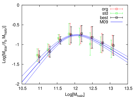
Figure 2: The fraction of baryons in the form of stars as a function of halo mass for model galaxies in the SAM+GCE with the best-fitting parameters ($x=1.1$ & $A=0.015$, black squares), with standard parameters ($x=1.3$ & $A=0.05$, green squares), and in the original SAM without GCE (red squares). The blue lines mark the empirical relation, and 1-$\sigma$ uncertainties, derived by Moster et al. (2009).

In Figure 3, we show the average star formation histories (SFH) of our model early-type galaxies, for galaxies with different present-day stellar masses. As pointed out in previous studies (see, e.g., De Lucia et al. 2006; S08; Trager & Somerville, 2009, hereafter TS09), SAMs with AGN feedback do qualitatively reproduce a downsizing-like trend (i.e., the higher mass galaxies have shorter SF timescales and less extended SFH). This is still true in our new models.

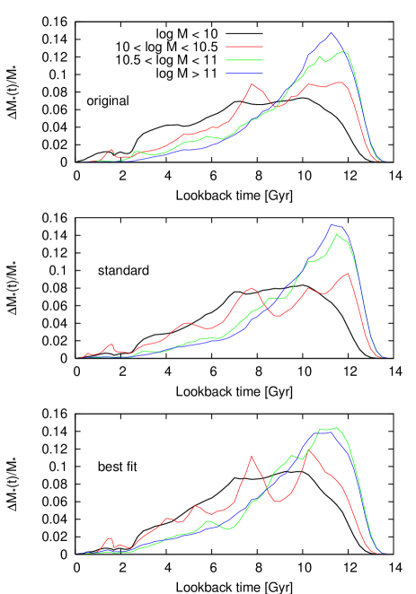
Figure 3: Smoothed average star-formation histories for model early-type galaxies in (from bottom to top) the SAM+GCE with the best-fitting parameters ($x=1.1$ & $A=0.015$), with standard parameters ($x=1.3$ & $A=0.05$), and in the original SAM without GCE, binned by the stellar mass of the galaxy at $z=0$.

Another very important observational quantity to reproduce is the colour-magnitude diagram (CMD) of galaxies. In Figure 4 we show magnitudes and colours of early-type galaxies in the SAM with and without GCE. Here there is one caveat regarding the calculation of the galaxy luminosities. The stellar population models that we use to predict the colours and magnitudes (Bruzual & Charlot, 2003) use a fixed standard Chabrier IMF, while we allow the slope of this IMF to change when calculating the chemical evolution. Although this is not self-consistent, such a minor change in the IMF parameters should not significantly affect the predicted colours or magnitudes since the early-type galaxies studied here are dominated by old populations for which high-mass stars are of little importance (C. Conroy, private communication). We divide the CMD into red and blue regions using the magnitude-dependent cut of Baldry et al. (2004). The galaxies form two clear groups: the majority in a bright red sequence and a few in a fainter blue cloud. The “original” and “best fit” models agree quite well with the observed CMD, while the luminous galaxies in the “standard model” are slightly too blue.

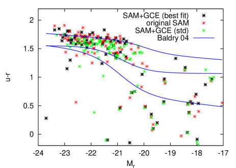
Figure 4: Colour-magnitude diagram (CMD) for model early-type galaxies in the SAM+GCE with the best-fitting parameters ($x=1.1$ & $A=0.015$, black stars), with standard parameters ($x=1.3$ & $A=0.05$, green stars), and in the original SAM without GCE (red stars). The blue lines mark, from top to bottom, the locus of the red sequence, the green valley and the blue cloud from Baldry et al. (2004).

In the previous version of the SAM, the fraction of cold gas relative to stars in galactic discs at the present time was used to calibrate the models by comparison with the observational estimates of Bell et al. (2003) for morphologically late-type galaxies (see Figure 5 in S08). This property is well reproduced by all test cases after implementing the GCE. Here we also compare the gas fraction of our galaxies, both early-type and discs, with those from Kannappan (2004) as a function of $u-r$ colour, as shown in Figure 5. The agreement in the slope, scatter and zero-point of the relation is quite good for all models, especially when the new model of galactic chemical evolution is included.

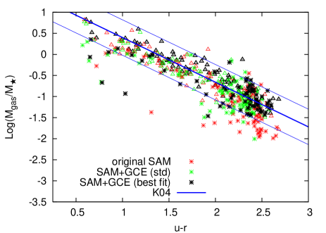
Figure 5: The gas fraction for model galaxies in the SAM+GCE with the best fitting parameters ($x=1.1$ & $A=0.015$, black symbols), with standard parameters ($x=1.3$ & $A=0.05$, green symbols), and in the original SAM without GCE (red symbols) as a function of $u-r$ colour. Stars and triangles depict early-type and disc galaxies, respectively. The thick blue line marks the median of the sample from Kannappan (2004), and the thin lines mark the $1-\sigma$ deviation.

The first evidence for the mass-metallicity relation can be seen when looking at the metallicity distribution function of galaxies of different masses, which we show in Figure 6 for our three test cases. All of the models agree qualitatively, showing an increasing mean of the distribution as the mass range increases. At a given mass, however, the distributions for the best-fitting model are shifted to higher metallicities since galaxies in this simulation are more metal rich (see below).

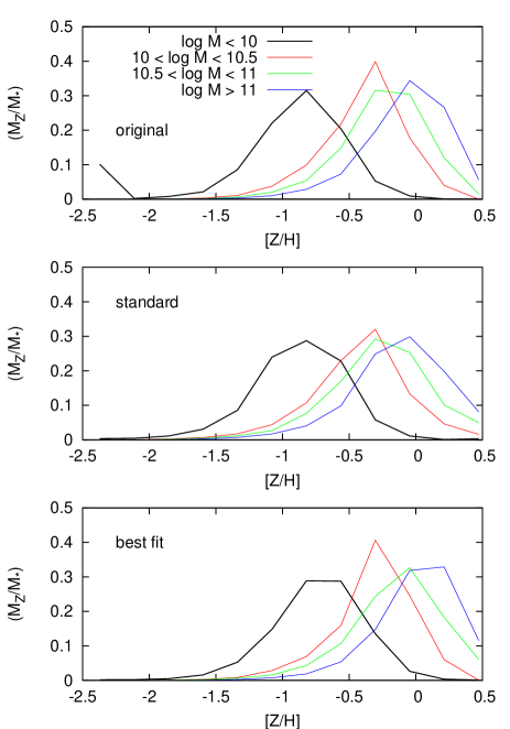
Figure 6: Average metallicity distributions for model early-type galaxies in (from bottom to top) the SAM+GCE with the best fitting parameters ($x=1.1$ & $A=0.015$), with standard parameters ($x=1.3$ & $A=0.05$), and in the SAM without GCE, binned by stellar mass.

Summarising, we have seen that including a detailed chemical evolution model in the SAM has a minor effect on the predicted formation histories and present-day properties of galaxies, and therefore does not require a re-calibration of the free parameters of the model. In the next subsection we will investigate the predicted metallicities and abundances, which are indeed affected by the GCE.

4.2 Chemistry of Early-type Galaxies

The main effect of the new treatment of chemical evolution is reflected in the metallicity and abundance ratios of the galaxies. Most SAMs reproduce fairly well the mass-metallicity relation of galaxies (with effective yield treated as a free parameter), but to date they have been unsuccessful in fitting the slope of the mass–[$\alpha$/Fe] relation (e.g., Nagashima et al., 2005b; Pipino et al., 2008). This is the main challenge that we address in this study.

The galaxy sample used for comparison is that described in Trager et al. (2000a). This sample has been reanalysed using the updated stellar population synthesis method presented in Trager et al. (2008), which is sensitive to age, metallicity and abundance ratios. In the current study, we use models based on the Bruzual & Charlot (2003) models with index variations due to abundance ratios taken from Lee et al. (2009). Inferred stellar population parameters are tabulated in Appendix B. When making the comparisons, we use the stellar mass of the simulated galaxies and the inferred dynamical mass of the observed ones. This should not introduce a significant bias since the dynamical mass is a good tracer of the stellar mass within one effective radius for most early-type galaxies (Cappellari et al., 2006). The abundances presented here were normalised to the solar values from Grevesse et al. (1996). We have also computed the present epoch SNe Ia and II rates for our galaxies and compared them with the results of Mannucci et al. (2005) and Sullivan et al. (2006).

4.2.1 Dependence on IMF slope and SN Ia fraction

In Figures 7 and 8 we show the relation between total metallicity ([Z/H]) and stellar mass ($M_{\star}$). From these figures, we see that in the “old” SAMs, galaxies tended to be too metal-poor compared to the observations (as seen in TS09), and implementing the detailed chemical evolution with the standard IMF improves the results only slightly. We explore the parameter space of the GCE equations to see if it is possible to improve the agreement with the observations. Specifically, the parameters allowed to vary are the fraction of binaries that give rise to SNe Ia ($A$ in Eq. 9), the slope of the IMF above $1\,M_{\sun}$ ($x$ in Eq. 11) and the upper mass limit of the IMF ($M_{U}$ in Eq. 9). However, we will only show the results for $M_{U}=40\,M_{\sun}$ for the following reason. Given that our chosen SN II yields (WW95) are only tabulated up to that value, we are forced to assume that the yields relative to the initial mass remain constant and equal to those of a $40\,M_{\sun}$ star for stars above this value when running simulations with higher upper mass limits. This proves to be an unreliable assumption, as reflected for example in the non-monotonic behaviour of the [$\alpha$/Fe] ratio as a function of the stellar mass of our galaxies, in serious disagreement with observations. Other properties, such as the SNe Ia rate, are not significantly affected by this parameter, as expected.

We also note that, even though we have varied the slope of the IMF, the supernova feedback efficiency remains the same because the prescription for the SN feedback energetics and the SN chemical enrichment are decoupled; the SN feedback efficiency is set manually as a free parameter (see Eq. 3), independent of the IMF. In this sense, the model is not entirely self-consistent. However, this choice makes it easier to interpret the effect of changing the IMF in the models.

We now compare the predictions for the observed galaxy sample, the original SAM, and the new SAM with GCE with a standard Chabrier IMF, a shallower IMF ($x=1.1$) and two choices of the parameter $A$ (0.015 and 0.05). The use of a shallower IMF results in an upwards shift in the zero-point of the mass-metallicity relation, bringing it into much better agreement with the observations. This increase in metallicity with a shallower IMF is expected since more massive stars are produced and therefore the gas is enriched more efficiently. The metallicities of the model galaxies show almost no dependence on the parameter $A$, which is not surprising since this parameter mainly controls the ratio of type Ia to type II supernovae, affecting abundance ratios but not the overall metallicity (in essence the production of $\alpha$-elements and Fe-peak elements compensate for one another).

Figure 7: The relationship between metallicity and stellar mass for the galaxies in our simulations and in the observational sample of T00. Symbols – pink squares: original SAM; red crosses: SAM+GCE with $x=1.3$ and $A=0.015$; blue crosses: SAM+GCE with $x=1.3$ and $A=0.05$; black stars with error bars – galaxies from Trager et al. (2000a), reanalysed as described in the text. Note the poor agreement of the model galaxies with the observations in all cases.

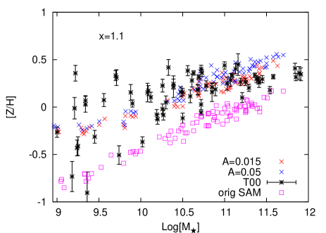
Figure 8: As in Figure 7, except with a shallower high-mass slope for the IMF ($x=1.1$) used in the SAM+GCE. Note the significantly better agreement of the model galaxies with the observations.

A primary advantage of our new model is that we can now calculate abundance ratios for our galaxies, which gives us yet another property to compare with observations and set further constraints on the models. This is shown in Figures 9 and 10, where we plot the [$\alpha$/Fe] ratio against stellar mass for the same parameter choices as before. For the simulated galaxies, we consider the abundance of $\alpha$-elements to be the composite abundance of N, Na, Ne, Mg, Si, and S (cf. Trager et al., 2000a). If we assume a value of the parameter $A\sim 0.05$ commonly used in the literature, the abundance ratios are far too low. The overall values of [$\alpha$/Fe] can be raised by decreasing the value of $A$ (i.e. producing fewer SNe Ia and consequently less iron). However, even with this decreased $A$ and the standard IMF, we see that the relation is too flat or even has a slightly negative slope, and for the galaxies at the high mass end the [$\alpha$/Fe] ratio is insufficiently enhanced. On the other hand, a shallower IMF, combined with a lower value of $A$, produces model galaxies in far better agreement with observations. The flatter IMF increases the slope of the relation while a low $A$ brings up the zero-point. Moreover, it is interesting to note that lowering $A$ also increases the slope (at any fixed IMF). This small steepening of the [$\alpha$/Fe]-mass relation is due to the metallicity dependence of the yields, since the higher the initial metallicity, the higher the [$\alpha$/Fe] in the yields. A lower fraction of SNe Ia (and consequently more type II) implies a slightly faster overall enrichment, and therefore galaxies spend more time forming stars in a regime of enhanced [$\alpha$/Fe] (higher metallicity yields).

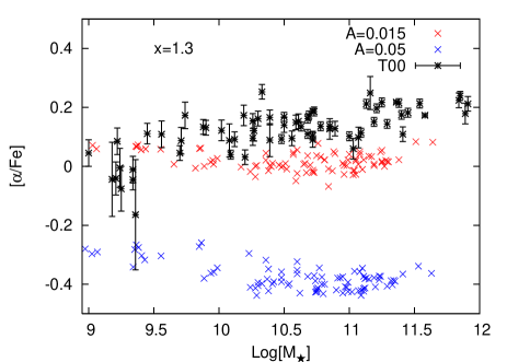
Figure 9: Relation between the [$\alpha$/Fe] ratio and stellar mass. Symbols – red crosses: SAM+GCE with $x=1.3$ and $A=0.015$; blue crosses: SAM+GCE with $x=1.3$ and $A=0.05$; black stars with error bars: galaxies from Trager et al. (2000a), reanalysed as discussed in the text. Note again the poor agreement of the model galaxies with the observations.

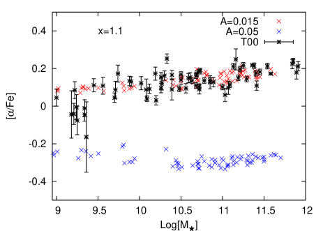
Figure 10: As in Figure 9, except $x=1.1$ for the model galaxies from the SAM+GCE. Note the better agreement with observations when using a low value of the SN Ia fraction $A$.

In summary, we had expected that the inclusion of AGN feedback in the semi-analytic models might solve the problems that previous studies have encountered in trying to reproduce the observed trend between mass and [$\alpha$/Fe] ratio, because the quenching due to AGN does lead to more massive galaxies having shorter formation timescales in the models. However, apparently the effect of “downsizing” on the trend of [$\alpha$/Fe] is very small and a flatter IMF is required to achieve agreement between the models and the observations. This does not undermine the potential importance of AGN feedback, which appears to be a promising mechanism for solving many of the other problems experienced by earlier generations of models (such as the overcooling problem). In any case, it is encouraging that with minor variations (within the observational uncertainties) in the chemical evolution parameters, we can for the first time obtain very good agreement with the observed mass-[$\alpha$/Fe] in a semi-analytic model.

One concern is that the comparison between our models and the observations is not strictly rigorous since we are showing stellar mass-weighted abundances for the models, while stellar population studies derive abundances from line-strength indexes from integrated spectra, which are themselves light-weighted quantities. However, TS09 have shown that the SSP-equivalent (absorption-line-weighted) metallicity correlates very well with its mass-weighted and light-weighted counterparts. In future work, nevertheless, we will synthesise line strengths for the galaxies in our simulations and calculate abundance ratios in the same way as is done in the observational data. One additional worry is the effect of limited aperture size on the comparison, as early-type galaxies are well-known to have significant line-strength gradients. These gradients imply however mild metallicity gradients but no abundance ratio gradients whatsoever (e.g., Davies et al., 1993; , Mehlert et al.2003; Sánchez-Blázquez et al., 2007, TS09). Therefore we are confident that trends in $[\alpha/\mathrm{Fe}]$ with mass are trustworthy. We note here (as described in Appendix B) that the data plotted in the figures have been constructed to appear as if the galaxies were at the distance of the Coma cluster and observed through fibre apertures of diameter $2\aas@@fstack{\prime\prime}7$ (see Trager et al., 2008). While this does not eliminate gradient effects on the inferred metallicities, it reduces their magnitude to an offset of roughly $-0.1$ dex (TS09).

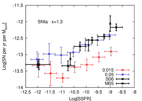
Figure 11: Present day SN Ia rate as a function of specific SFR. Here we show all model galaxies, regardless of morphology. Red stars are SAM+GCE with $x=1.3$ and $A=0.015$; blue stars SAM+GCE with $x=1.3$ and $A=0.05$; black squares are observations from Sullivan et al. (2006) and black crosses from Mannucci et al. (2005). The conversion of galaxy type into specific SFR for the Mannucci et al. data points is the same as in Sullivan et al. (2006).

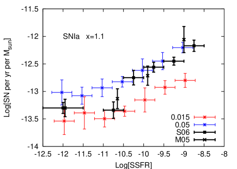
Figure 12: As in Figure 11, except using the shallower IMF ($x=1.1$) for the model galaxies from the SAM+GCE.

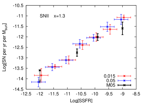
Figure 13: Present-day SN II rate as a function of SSFR. Symbols are as in Figure 11. Results are shown for the standard IMF ($x=1.3$). We remind the reader that the upper-mass limit on the IMF is $40\,M_{\sun}$

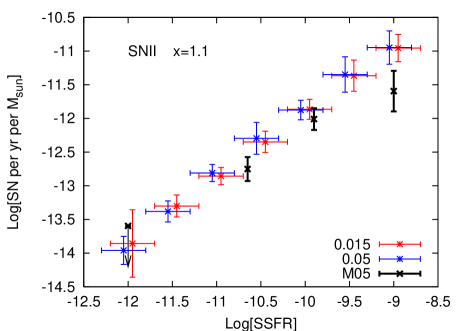
Figure 14: The same as Figure 13, except we use the shallower IMF slope ($x=1.1$) for the model galaxies from the SAM+GCE.

Supernovae rates provide further independent constraints our models. We calculate the predicted supernovae rates for our model galaxies and compare them with those derived by Mannucci et al. (2005) and Sullivan et al. (2006) for a large sample of galaxies in the nearby universe. In Figures 11 and 12 we show the present day type Ia supernova rate in units of SN events per year per unit stellar mass versus the specific star formation rate (SSFR, star formation rate per unit stellar mass), and in Figures 13 and 14 we show the rates for Type II SNe. Here we show all the model galaxies regardless of morphology, since the early-type galaxies populate only the lower SSFR side of these diagrams, and both comparison samples include galaxies of all morphological types. The galaxies in these sample are from a mixture of field and small cluster environments, but so are our model galaxies.

The slope of the IMF has little effect on the predicted SNIa rates; only the $A$ parameter has a significant influence on the results. From Figures 11 and 12, we see that no combination of IMF slope and fraction of binaries that yield SNe Ia can fit the observations over the whole range of SSFR. However, it is interesting to notice that SNe Ia rates of star forming galaxies (SSFR $>10^{-10.5}$) are very well matched by models with a high value of $A$, while a low value of $A$ is a better match for passive galaxies (SSFR $<10^{-10.5}$). This behaviour, which is seen regardless of the slope of the IMF, is almost certainly due to the chosen supernova Ia model. In the Greggio & Renzini (1983) formalism which we use, the Delay Time Distribution (DTD) of the SN Ia explosions is given by a convolution of the distribution of secondary masses (in binary systems) and the lifetime of the secondary star. On the other hand, from the same observational data, Mannucci et al. (2006) derived a DTD with two components: a prompt peak and a later plateau, each encompassing half of the SNe Ia. Other authors have also reached similar conclusions about the delay-time distribution of type Ia explosions (e.g. Scannapieco & Bildsten, 2005; Dahlen et al., 2008). This bimodal DTD effectively enhances the production of type Ia supernovae in star forming galaxies, exactly where a higher fraction of SNIa are needed in our models. We therefore expect that using a two-population DTD with a significant prompt component will alleviate the differences between our model predictions and the observed Type Ia rates, and we show that this is the case below.

The Type II SN rates, on the other hand, show very good agreement with the observations over the whole range of SSFR. In this case, all variations of $x$ and $A$ give the same qualitative results, although the models with the “standard” parameter values are slightly better. Nevertheless, as we have shown above, not all combinations of IMF slopes and values of $A$ (SN Ia producing fraction of binaries) produce model galaxies that agree with observed metallicities and abundance ratios. It is only for those models with a shallower IMF ($x\sim 1.1$) and lower SNe Ia fraction among binaries ($A\sim 0.01$–0.02) that we can reasonably reproduce the full set of observations.

To summarise, after implementing detailed chemical evolution in the semi-analytic model of S08, we can now reproduce the mass–metallicity and mass–[$\alpha$/Fe] relations for local early-type galaxies, provided we use a slightly flatter Chabrier IMF and a low fraction of binaries giving rise to SN Ia. The predicted rates of Type Ia SNe show a strong dependence on the fraction of binaries that yield such an event (our parameter $A$) but not on the slope of the IMF, with the rates in star forming galaxies better matched by a high value of $A$, while those in passive galaxies are better with a low value of A. However, for a standard IMF and high value of $A$, the galaxies are a bit too metal-poor and, most importantly, the abundance ratios are extremely low, in severe disagreement with observations.

4.2.2 Bimodal Delay Time Distribution for Type Ia Supernovae

In the previous section, we speculated that a bimodal distribution with a prompt population of SNe Ia explotions would give a better match for the observed supernova rates. Given the analytical nature of the DTD formulation (Greggio, 2005), it is fairly straightforward to implement and test this hypothesis. We have implemented the DTD proposed by Mannucci et al. (2006). Figure 15 shows the four observational constraints used to test the models (metallicity vs. stellar mass, [$\alpha$/Fe] vs. stellar mass, type Ia SNR vs. SSFR, and type II SNR vs. SSFR). Clearly the new double-peaked SN Ia DTD model gives a better match to the Type Ia SN rates, while maintaining the good agreement in the other galactic properties. However, for this model, the best-fitting parameters for the IMF slope and the SNIa binary fraction are slightly different; specifically, $x=1.15$ and $A=0.03$. This value for the IMF is in even better agreement with some recent studies (Baldry & Glazebrook, 2003; , Wilkins et al.2008) then our previous ‘best’ value of $x=1.1$.

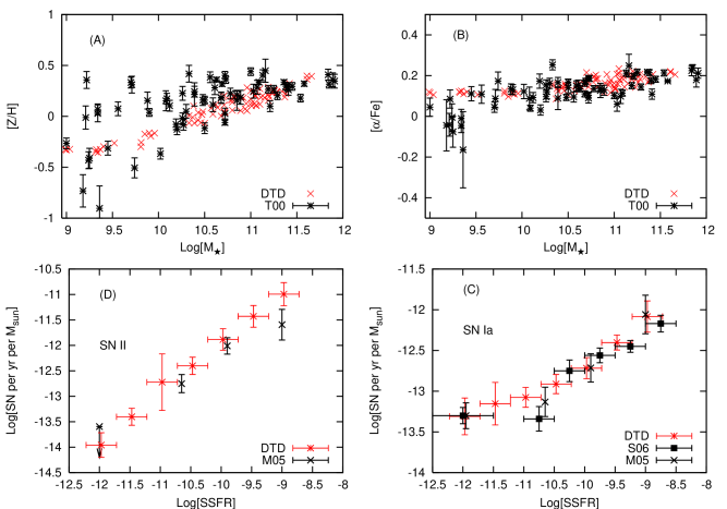
Figure 15: Clockwise, starting from the top left panel: (A) [Z/H] vs. stellar mass; (B) [$\alpha$/Fe] vs. stellar mass; (C) Type Ia SNR vs. SSFR; (D) Type II SNR vs. SSFR. Symbols – red crosses: SAM+GCE with bimodal DTD for SNe Ia ($x=1.15,\,A=0.03$); T00: reanalysed metallicities and abundance ratios from Trager et al. (2000a), M05 and S06: SN rates from Mannucci et al. (2005) and Sullivan et al. (2006) respectively.

Finally, in Figure 16 we show the abundance ratios of some individual elements for the galaxies in our best fitting models using the classic SNe Ia recipe ($x=1.1$ and $A=0.015$) and the bimodal DTD ($x=1.15$ and $A=0.03$). With the exception of C and N, which are slightly higher for the latter, all the elements follow the same trends in both models. In particular Mg, even though it is under-abundant with respect to other $\alpha$-elements, is the one element that best follows the observed trend of [$\alpha$/Fe]. This leads us to believe that the abundances derived from the stellar population analysis may be predominantly driven by Mg, and may not necessarily reflect of all the $\alpha$-elements. There is also an excess of Ni in the Fe-peak group and a decreasing trend of [C/Fe] with increasing galactic mass which is apparently not observed (Sánchez-Blázquez et al., 2003; Graves & Schiavon, 2008). This should not be considered a flaw of the model, since the abundances of individual elements are very sensitive to the chosen yields. We expect that future line-strength observations, interpreted with next-generation stellar population models (such as Schiavon, 2007; Lee et al., 2009), will provide an interesting test of our models, including the set of assumed yields (KL07 + WW95 + N97).

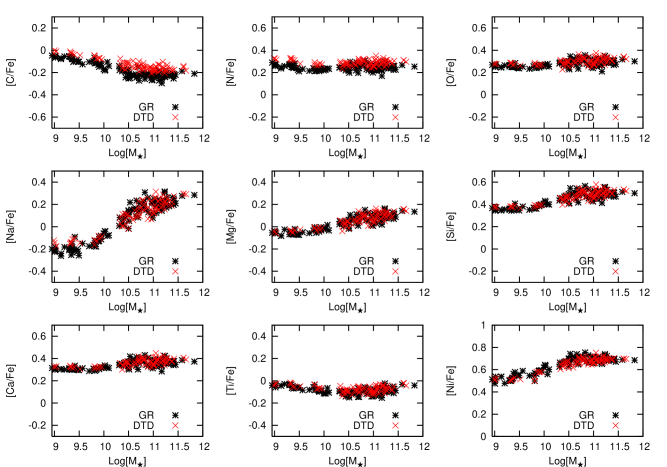
Figure 16: [el/Fe] versus stellar mass for some $\alpha$-elements and Fe-peak elements. Only predictions from our best-fitting models are shown. Symbols – black stars: Classic SN Ia (Greggio & Renzini, 1983); red crosses: DTD formulation (Greggio, 2005). The parameters are ($x=1.1$, $A=0.015$) and ($x=1.15$, $A=0.03$) respectively.

4.2.3 Dependence on other model parameters

We have also explored whether we could match the observations investigated above by varying the galaxy formation parameters of the SAM instead of the IMF and binary fraction parameters. For this purpose, we ran several simulations in which we modified the star formation efficiency ($A_{K}$ in Eq. 2), the SN feedback efficiency ($\epsilon_{0}^{SN}$ in Eq. 3) and the virial velocity below which ejection of reheated gas from the halo into the diffuse intergalactic medium becomes important ($V_{\mathrm{eject}}$ in Eq. 4). When the star formation efficiency was increased by a constant factor, a few more massive galaxies were produced and the slope of the mass–[$\alpha$/Fe] relation increased slightly but the slope and zero point of the mass–metallicity relation did not change. A higher SF efficiency implies that the cold gas is consumed more rapidly and therefore the timescale for star formation is shorter, which is why the mass–[$\alpha$/Fe] relation was affected.

If $A_{K}$ was allowed to increase with increasing galactic baryonic mass, a considerable number of very massive galaxies were produced and the slope of the mass–metallicity relation increased mildly (but not the zero point). On the other hand, if the factor decreased with increasing galactic mass, the trends remained the same but no galaxies above $10^{11}\,M_{\sun}$ were produced. This excess or lack of high mass galaxies arises because star formation in the biggest systems is either boosted or suppressed by this mass-dependent variation of the SF efficiency.

The effects of reducing the SN feedback efficiency and the $V_{\mathrm{eject}}$ parameter were roughly the same. In both cases the slope and zero point of the mass–metallicity relation increased slightly and the central galaxies of the DM haloes were on average more massive, but the mass–[$\alpha$/Fe] relation did not change and an unrealistically large number of low-mass satellite galaxies was also produced. This excess of low-mass satellites is due to the fact that small galaxies retain their gas more efficiently when these parameters that control the SN feedback are decreased.

Overall, the effect of changing these other parameters is not as strong as flattening the IMF, and also destroys the agreement with other well-calibrated observations, such as the luminosity function, the metallicity distribution function, and the cold gas fraction. We therefore conclude that our results are robust to the values of these free parameters.

As a final test, we modified some of the yields. Specifically, we decreased the Fe yield of SNe II by half and increased the Mg yield by a factor of four. Reducing the Fe yield had very little effect, indicating that the bulk of the Fe comes from SNe Ia, as expected. Changing the Mg yield raised the zero point of the relations, as expected. However, neither of these changes affected the slope. Pipino et al. (2008) reached a similar conclusion about the yields and other parameters when exploring the parameter space in their models.

5 Discussion and Conclusions

We have implemented detailed galactic chemical evolution in a semi-analytic model, and use the resulting model to study the metal enrichment of early type galaxies in the local universe. The base SAM is that presented in Somerville et al. (2008). We take into account the effects of galaxy mergers, inflow of cold gas, and SN and AGN driven outflows, as well as the production of metals by SN Ia, SN II and AGB stars. Unlike most previous SAMs we discard the instantaneous recycling approximation by properly accounting for the finite lifetimes of the stars and also make use of metallicity dependent yields.

We run our SAM+GCE simulations in a grid of dark matter haloes ranging over present-day masses of $10^{11}$ to $10^{13}\,M_{\sun}$. We allow the slope of the IMF and the fraction of binaries that produce a SN Ia event to vary, and compare our results with the observed trends of metallicity and abundance ratio ([$\alpha$/Fe]) against stellar mass of the galaxies, as well as the supernova rate (both type Ia and II) as a function of specific star formation rate. Only the models with a shallow IMF ($x=1.1$) and a low fraction of SN Ia from binaries ($A\sim 0.015$) match all four observations of early-type galaxies simultaneously. A slightly flatter than standard IMF is necessary in order to produce more massive stars, which enrich the interstellar medium more efficiently, making the galaxies in our simulations become more metal rich and improving the agreement with the data. The production of more massive stars, along with the fact that the star formation histories are more extended in time as the galaxy mass decreases, helps to achieve the correct trend of increasing [$\alpha$/Fe] with increasing galaxy stellar mass. However, it is also necessary to invoke a low fraction of SNe Ia to raise the zero-point of this relation. We also predict abundance patterns for a variety of elements for early-type galaxies at $z=0$ in our fiducial model. These predictions will be interesting to compare with future observations.

From studying the SNe Ia rates, we find evidence supporting a ‘two-population’ distribution for the type Ia explosions, since galaxies with high specific star formation rates are better matched by models with a high fraction of binaries that explode as SN Ia ($A$) while those with low SSFR require a low value of $A$. We tested whether the use of a more realistic (bimodal) delay-time distribution of type Ia supernovae would, in fact, improve the results. After implementing the DTD formulation for SNe Ia and using a bimodal distribution with a prompt peak and an extended plateau, we found very good agreement with the SN rates, while still matching the trends of [Z/H] and [$\alpha$/Fe] with stellar mass, although the best values for the slope of the IMF changed slightly and the fraction of SNeIa binaries needed to be doubled. Our favored model is now one with a Chabrier-like IMF with a slope of $x=1.15$, a SNe Ia binary fraction of $A=0.03$ (relative to the $3-16\,M_{\sun}$ range, $A\sim 0.0014$ relative to the full range of masses defining the IMF), and a bimodal delay-time-distribution for Type Ia SN events as proposed by Mannucci et al. (2006).

We have also studied the effects of varying the galaxy formation parameters in the SAM, but found that we were unable to reproduce the observations in this way. We therefore conclude that our results are robust to the values of the free parameters in the SAM.

This is not the first time that a GCE model has been applied within a SAM. Nagashima et al. (2005a, b) have also constructed such a model, and their ‘superwind’ model resembles our model. They first obtained fairly good agreement with observations of ICM abundances in galaxy clusters, however the same models failed to reproduced the trend of increasing [$\alpha$/Fe] with increasing galactic mass. One of the main differences between their models and ours is in fact the IMF. They use a Kennicutt IMF ($x=1.5$) for quiescent star formation and a flat IMF ($x=0.0$) for stars formed in bursts. This flat IMF is rather extreme, while the proposed modification in our models is small, in fact within the observational uncertainties. Namely, we require the same ‘shallow’ IMF ($x=1.15$) for all modes of star formation. Another model that reproduces the observed scaling of abundance ratio with galaxy mass is that of Pipino & Matteucci (2004, 2006). However they consider a very different scenario for galaxy formation, the monolithic collapse scenario, and allow for galaxy mergers only in the form of a second infalling episode. More recently, Pipino et al. (2008) also coupled GCE to a SAM, but they also failed to match the mass–[$\alpha$/Fe] relation. They claim that flattening the IMF can not solve this problem, in contradiction with our findings. It is worth mentioning that none of these models include AGN feedback; only the GalICS model used by Pipino et al. (2008) has some form of halo quenching simply by shutting down the flow of cold gas onto galaxies with masses larger than $10^{11}\,M_{\sun}$. However, contrary to our expectations, we find that SF quenching by AGN is not a key factor in our success at reproducing the mass–[$\alpha$/Fe] relation, even though the AGN feedback in our models leads to shorter formation times for the more massive galaxies. We find that a slight flattening of the IMF is essential to achieve agreement between the model and the observations. AGN feedback, nonetheless, is likely to play an important role in reproducing other galaxy observations, such as the stellar mass or luminosity function and color bimodality.

Our best-fitting IMF, nonetheless, is consistent with observations; the slope is within the observational uncertainty of Chabrier (2003) and agrees remarkably well with the results of Baldry & Glazebrook (2003), who found that ultraviolet to near-infrared galaxy luminosity densities require an IMF with a slope of $1.15\pm 0.2$. The same slope was found by (Wilkins et al.2008) when trying to reconcile the redshift evolution of the observed stellar mass density with the cosmic SFH using a constant and universal IMF. The agreement, however, holds only at low redshift. In a forthcoming paper, Wilkins et al. (in preparation) propose an evolving IMF as a plausible solution. Such an IMF should be strongly top-heavy at high redshift (Hopkins, private communication). van Dokkum (2008) also suggests an evolving Chabrier-like IMF based on comparing the evolution of the $M/L$ ratios of early-type galaxies to their colour evolution, but in this case the change is in the characteristic mass ($m_{c}$ in Eq. 11) rather than the slope, making the IMF “bottom-light” at high redshift. Such evolving IMFs could, in principle, work in favour of the trends of [$\alpha$/Fe] with stellar mass and SNR with SSFR since they produce either more SN II or fewer SN Ia progenitors at earlier times when massive early-type galaxies create most of their stars. This scenario remains to be tested, and moreover the issue of an evolving IMF is open to considerable debate given the large uncertainties on its constraints. On a different note, Meurer et al. (2009) has claimed evidence for an IMF that depends on galactic surface brightness (or surface density) as a plausible explanation for an observed variation in H_α/FUV flux ratio. However, they invoke variations that are an order of magnitude larger than the deviation of our best-fitting slope from the standard value. Finally, very recently, Calura & Menci (2009) have claimed that a constant IMF cannot account for the trends of [Z/H] and [$\alpha$/Fe] with velocity dispersion in elliptical galaxies and have proposed an IMF with a slope depending on the SFR ($x=1.35$ for low star-forming systems and $x=1$ for high star-forming systems) in order to explain them. However, their chemical evolution is not coupled to a semi-analytic model, but is computed a posteriori with SFHs extracted from the SAM of Menci et al. (2008), and therefore the flows of enriched gas from the galaxies into the halos and back again are not tracked, unlike in the our model.

In future work we will apply this model to other questions such as the abundances of different components of spiral galaxies like the Milky Way (e.g. the disk, bulge, and stellar halo), abundances in clusters vs. the field, abundances in the intra-cluster gas, and to the evolution of metals over cosmic time.

Appendix A Implementation Algorithm of the GCE modelling

Table 1: Structure of the grid where the star formation and abundance histories are stored. All quantities are in Gyr.

Age Range	Size of bins
0.00 – 0.12	0.01
0.12 – 0.40	0.02
0.40 – 1.12	0.04
1.12 – 2.72	0.08
2.72 – 11.68	0.32
11.68 –	1.28

The initial size of the bins is 0.01 Gyr because it is the maximum possible value of the time-step in our simulations.

To compute the chemical enrichment consistently as described in Section 2, it is imperative to keep track of the star formation history of each galaxies as well as the metallicity of the ISM as a function of time in these galaxies. Given the large number of galaxies in the simulations, it is very expensive, both in computing time and in physical memory, to store these quantities in a linear time grid with reasonable resolution. In order to overcome these limitations, we use an age grid where first bin of this grid represents $t=t_{\mathrm{now}}$ at any moment during the calculations and the size (in time) of the bins increase as we go to older ages. The scaling of the bins is related to the lifetimes of the stars, so that it increases as the lifetimes of the stars become progressively larger. The size of the bins only increases, but each subsequent bin is not necessarily larger than the previous one. In Table 1 we show the structure of this binning grid. In this grid we store the amount of cold gas mass turned into stars, $\Delta M_{\star}$, and the metallicity of the cold gas, $Z_{g}$. As the systems evolve this information is ‘pushed down’ to older bins, directly if the subsequent bin is of the same size or added if the bin is of a larger size. In the later case, the cold gas masses are added directly whereas the the metallicity is averaged, weighted by the size of the bins. In essence, what we extract from this grid are time-averaged quantities.

It is also important how we handle this information when galaxies merge, that is, how we combine the star formation and metallicity histories of the merging galaxies. This is done on a bin-by-bin basis. At a given age bin, $\Delta M_{\star}$ is added directly and the metallicities are averaged weighted by the corresponding $\Delta M_{\star}$. In mathematical form,

$$\Delta M_{\star}[i] = \Delta M_{\star}^{A}[i]+\Delta M_{\star}^{B}[i],$$ (17)

$$Z_{g} = \frac{Z_{g}^{A}*\Delta M_{\star}^{A}[i]+Z_{g}^{B}\Delta M_{\star}^{B}[i]}{\Delta M_{\star}^{A}[i]+\Delta M_{\star}^{B}[i]},$$ (18)

where $A$ and $B$ are the merging galaxies and $i$ the age bin. Summarising, the star formation rate and the cold gas metallicity used in Eq. 9 to calculate the enrichment of the ISM are average quantities.

Appendix B Galaxy Sample

The sample of galaxies used to test our models was taken from Trager et al. (2000a) and reanalysed with the method described in Trager et al. (2008). Specifically, we used the Bruzual & Charlot (2003) stellar population models and modified the line strengths when $[\alpha/\mathrm{Fe}]\neq 0$ using ‘response functions’ that have been calculated for each star in each isochrone, a significant improvement over previous methods (e.g., Tripicco & Bell, 1995; Korn et al., 2005). More details can be found in Trager et al. (2008) and Lee et al. (2009). In Table 2 we present the results from this new stellar population synthesis analysis.

We also present dynamical mass computed using

$$M_{\mathrm{dyn}}=465\sigma^{2}r_{e},$$ (19)

where $\sigma$ is the central velocity dispersion in $\mathrm{km\,s^{-1}}$ (here we use the velocity dispersion taken through an aperture of diameter $r_{e}/8$) and $r_{e}$ is effective radius in parsecs (see Trager et al., 2000b, for more details).

Table 2: Velocity dispersions, ages, metallicities, enhancement ratios and dynamical masses of the sample galaxies.

Galaxy	Type	Log($\sigma$)	log(Age)	[Z/H]	[E/Fe]	$\log(M_{\mathrm{dyn}})$
ESO358-G06	S0	$1.763\pm 0.072$	$0.807_{-0.250}^{+0.114}$	$-0.431_{-0.098}^{+0.083}$	$-0.005_{-0.045}^{+0.066}$	$9.24\pm 0.43$
ESO358-G25	S0	$1.690\pm 0.072$	$0.779_{-0.295}^{+0.326}$	$-0.732_{-0.144}^{+0.159}$	$-0.044_{-0.096}^{+0.126}$	$9.18\pm 0.39$
ESO358-G50	S0	$1.732\pm 0.072$	$0.707_{-0.235}^{+0.129}$	$-0.412_{-0.098}^{+0.098}$	$-0.076_{-0.056}^{+0.076}$	$9.25\pm 0.48$
ESO358-G59	S0	$1.653\pm 0.072$	$0.544_{-0.068}^{+0.235}$	$-0.266_{-0.114}^{+0.053}$	$0.045_{-0.035}^{+0.045}$	$9.00\pm 0.45$
ESO359-G02	S0	$1.763\pm 0.072$	$0.603_{-0.189}^{+0.159}$	$-0.904_{-0.189}^{+0.220}$	$-0.164_{-0.500}^{+0.187}$	$9.36\pm 0.46$
IC1963	S0	$1.763\pm 0.072$	$0.397_{-0.068}^{+0.114}$	$0.357_{-0.098}^{+0.083}$	$0.085_{-0.035}^{+0.045}$	$9.22\pm 0.50$
IC2006	E	$2.134\pm 0.024$	$1.126_{-0.114}^{+0.098}$	$0.049_{-0.083}^{+0.068}$	$0.162_{-0.015}^{+0.025}$	$10.30\pm 0.33$
NGC0221	E	$1.731\pm 0.021$	$0.975_{-0.053}^{+0.068}$	$-0.398_{-0.038}^{+0.038}$	$-0.026_{-0.005}^{+0.025}$	$8.32\pm 0.28$
NGC0224	E	$2.185\pm 0.008$	$0.926_{-0.159}^{+0.129}$	$0.281_{-0.038}^{+0.068}$	$0.153_{-0.005}^{+0.025}$	$10.61\pm 0.15$
NGC0315	E	$2.486\pm 0.005$	$0.860_{-0.083}^{+0.098}$	$0.316_{-0.023}^{+0.038}$	$0.239_{-0.005}^{+0.015}$	$11.85\pm 0.35$
NGC0507	E	$2.445\pm 0.009$	$0.601_{-0.098}^{+0.129}$	$0.359_{-0.053}^{+0.068}$	$0.179_{-0.015}^{+0.035}$	$11.89\pm 0.34$
NGC0584	E	$2.278\pm 0.005$	$0.531_{-0.023}^{+0.053}$	$0.318_{-0.023}^{+0.023}$	$0.172_{-0.005}^{+0.015}$	$10.69\pm 0.30$
NGC0636	E	$2.185\pm 0.007$	$0.762_{-0.068}^{+0.098}$	$0.160_{-0.053}^{+0.053}$	$0.093_{-0.015}^{+0.015}$	$10.48\pm 0.34$
NGC0720	E	$2.381\pm 0.011$	$0.653_{-0.174}^{+0.326}$	$0.448_{-0.083}^{+0.114}$	$0.249_{-0.025}^{+0.056}$	$11.16\pm 0.27$
NGC0821	E	$2.281\pm 0.005$	$0.950_{-0.038}^{+0.068}$	$0.210_{-0.023}^{+0.038}$	$0.137_{-0.005}^{+0.015}$	$10.85\pm 0.28$
NGC0936	S0	$2.258\pm 0.026$	$1.110_{-0.098}^{+0.098}$	$-0.084_{-0.053}^{+0.053}$	$0.121_{-0.015}^{+0.035}$	$10.27\pm 0.42$
NGC1316	S0	$2.344\pm 0.024$	$0.510_{-0.053}^{+0.038}$	$0.260_{-0.038}^{+0.053}$	$0.109_{-0.015}^{+0.025}$	$11.41\pm 0.22$
NGC1336	E	$1.982\pm 0.024$	$1.073_{-0.068}^{+0.114}$	$-0.367_{-0.053}^{+0.053}$	$0.122_{-0.015}^{+0.035}$	$10.02\pm 0.31$
NGC1339	E	$2.199\pm 0.024$	$1.146_{-0.129}^{+0.098}$	$-0.079_{-0.053}^{+0.053}$	$0.173_{-0.015}^{+0.035}$	$10.19\pm 0.40$
NGC1351	E	$2.196\pm 0.024$	$1.129_{-0.083}^{+0.098}$	$-0.117_{-0.038}^{+0.053}$	$0.140_{-0.015}^{+0.025}$	$10.50\pm 0.31$
NGC1373	E	$1.875\pm 0.024$	$1.010_{-0.053}^{+0.083}$	$-0.313_{-0.083}^{+0.068}$	$0.111_{-0.015}^{+0.035}$	$9.45\pm 0.45$
NGC1374	E	$2.267\pm 0.024$	$0.931_{-0.068}^{+0.083}$	$0.114_{-0.114}^{+0.068}$	$0.149_{-0.015}^{+0.025}$	$10.59\pm 0.31$
NGC1375	S0	$1.748\pm 0.072$	$0.323_{-0.023}^{+0.023}$	$0.068_{-0.068}^{+0.053}$	$-0.045_{-0.025}^{+0.035}$	$9.34\pm 0.40$
NGC1379	E	$2.114\pm 0.024$	$0.913_{-0.053}^{+0.083}$	$-0.020_{-0.053}^{+0.053}$	$0.154_{-0.015}^{+0.025}$	$10.26\pm 0.32$
NGC1380	S0	$2.340\pm 0.024$	$1.008_{-0.083}^{+0.114}$	$0.157_{-0.068}^{+0.098}$	$0.127_{-0.015}^{+0.035}$	$10.85\pm 0.28$
NGC1380A	S0	$1.740\pm 0.072$	$0.476_{-0.083}^{+0.235}$	$-0.012_{-0.098}^{+0.114}$	$-0.041_{-0.035}^{+0.056}$	$9.21\pm 0.40$
NGC1381	S0	$2.185\pm 0.024$	$0.923_{-0.038}^{+0.068}$	$0.104_{-0.038}^{+0.053}$	$0.092_{-0.005}^{+0.025}$	$10.12\pm 0.39$
NGC1399	E	$2.574\pm 0.024$	$1.026_{-0.053}^{+0.083}$	$0.346_{-0.038}^{+0.068}$	$0.212_{-0.015}^{+0.025}$	$11.91\pm 0.21$
NGC1404	E	$2.415\pm 0.024$	$0.994_{-0.053}^{+0.068}$	$0.187_{-0.038}^{+0.068}$	$0.128_{-0.005}^{+0.025}$	$10.89\pm 0.32$
NGC1419	E	$2.068\pm 0.024$	$1.308_{-0.220}^{+0.220}$	$-0.506_{-0.189}^{+0.098}$	$0.173_{-0.025}^{+0.045}$	$9.74\pm 0.45$
NGC1427	E	$2.243\pm 0.024$	$0.981_{-0.023}^{+0.038}$	$-0.062_{-0.023}^{+0.023}$	$0.104_{-0.005}^{+0.015}$	$10.72\pm 0.29$
NGC1453	E	$2.475\pm 0.005$	$1.008_{-0.053}^{+0.053}$	$0.294_{-0.023}^{+0.038}$	$0.182_{-0.005}^{+0.015}$	$11.45\pm 0.39$
NGC1461	S0	$2.294\pm 0.011$	$0.864_{-0.098}^{+0.098}$	$0.155_{-0.053}^{+0.083}$	$0.134_{-0.015}^{+0.025}$	$9.88\pm 0.67$
NGC1600	E	$2.508\pm 0.009$	$0.822_{-0.114}^{+0.189}$	$0.409_{-0.023}^{+0.053}$	$0.224_{-0.015}^{+0.025}$	$11.84\pm 0.36$
NGC1700	E	$2.356\pm 0.005$	$0.519_{-0.008}^{+0.038}$	$0.335_{-0.023}^{+0.023}$	$0.114_{-0.005}^{+0.015}$	$11.09\pm 0.32$
NGC2300	E	$2.418\pm 0.006$	$0.719_{-0.144}^{+0.053}$	$0.404_{-0.023}^{+0.053}$	$0.212_{-0.005}^{+0.015}$	$11.13\pm 0.38$
NGC2560	S0	$2.303\pm 0.006$	$0.810_{-0.174}^{+0.159}$	$0.226_{-0.053}^{+0.068}$	$0.096_{-0.015}^{+0.025}$	$10.26\pm 0.94$
NGC2778	E	$2.198\pm 0.007$	$0.897_{-0.174}^{+0.098}$	$0.243_{-0.053}^{+0.053}$	$0.166_{-0.005}^{+0.025}$	$10.39\pm 0.35$
NGC3115	S0	$2.378\pm 0.053$	$0.574_{-0.068}^{+0.159}$	$0.384_{-0.053}^{+0.053}$	$0.095_{-0.025}^{+0.025}$	$10.56\pm 0.32$
NGC3377	E	$1.981\pm 0.009$	$0.653_{-0.098}^{+0.068}$	$0.038_{-0.038}^{+0.038}$	$0.131_{-0.005}^{+0.025}$	$9.90\pm 0.28$
NGC3379	E	$2.291\pm 0.005$	$0.969_{-0.023}^{+0.038}$	$0.159_{-0.023}^{+0.038}$	$0.168_{-0.005}^{+0.015}$	$10.50\pm 0.28$
NGC3384	S0	$2.140\pm 0.031$	$0.522_{-0.053}^{+0.083}$	$0.332_{-0.038}^{+0.053}$	$0.045_{-0.015}^{+0.025}$	$9.70\pm 0.44$
NGC3412	S0	$2.013\pm 0.034$	$0.632_{-0.159}^{+0.098}$	$0.029_{-0.083}^{+0.083}$	$-0.011_{-0.035}^{+0.045}$	$9.34\pm 0.49$
NGC3585	S0	$2.307\pm 0.122$	$0.710_{-0.159}^{+0.129}$	$0.247_{-0.053}^{+0.068}$	$0.060_{-0.015}^{+0.035}$	$11.03\pm 0.35$
NGC3607	S0	$2.332\pm 0.101$	$0.720_{-0.174}^{+0.189}$	$0.285_{-0.068}^{+0.068}$	$0.098_{-0.025}^{+0.035}$	$11.07\pm 0.33$
NGC3608	E	$2.259\pm 0.006$	$0.930_{-0.083}^{+0.083}$	$0.224_{-0.038}^{+0.053}$	$0.136_{-0.005}^{+0.015}$	$10.78\pm 0.28$
NGC3818	E	$2.246\pm 0.007$	$0.763_{-0.068}^{+0.144}$	$0.361_{-0.023}^{+0.038}$	$0.186_{-0.005}^{+0.015}$	$10.73\pm 0.35$
NGC3941	S0	$2.117\pm 0.036$	$0.422_{-0.098}^{+0.083}$	$0.311_{-0.098}^{+0.083}$	$0.087_{-0.035}^{+0.045}$	$9.71\pm 0.42$
NGC4026	S0	$2.258\pm 0.029$	$0.542_{-0.083}^{+0.159}$	$0.153_{-0.083}^{+0.098}$	$0.088_{-0.035}^{+0.056}$	$10.08\pm 0.41$
NGC4036	S0	$2.220\pm 0.039$	$0.574_{-0.129}^{+0.114}$	$0.418_{-0.038}^{+0.083}$	$0.253_{-0.015}^{+0.025}$	$10.33\pm 0.45$
NGC4111	S0	$2.127\pm 0.019$	$0.464_{-0.008}^{+0.023}$	$0.074_{-0.083}^{+0.068}$	$0.109_{-0.035}^{+0.045}$	$9.56\pm 0.56$
NGC4251	S0	$2.072\pm 0.074$	$0.514_{-0.038}^{+0.038}$	$0.173_{-0.038}^{+0.053}$	$0.040_{-0.015}^{+0.015}$	$10.09\pm 0.38$
NGC4261	E	$2.479\pm 0.005$	$1.136_{-0.053}^{+0.053}$	$0.284_{-0.023}^{+0.038}$	$0.175_{-0.005}^{+0.015}$	$11.40\pm 0.28$
NGC4697	E	$2.211\pm 0.009$	$0.924_{-0.053}^{+0.068}$	$0.027_{-0.038}^{+0.053}$	$0.090_{-0.005}^{+0.025}$	$10.72\pm 0.23$
NGC5638	E	$2.186\pm 0.006$	$0.946_{-0.038}^{+0.068}$	$0.185_{-0.023}^{+0.053}$	$0.162_{-0.005}^{+0.015}$	$10.68\pm 0.29$
NGC5812	E	$2.300\pm 0.005$	$0.602_{-0.114}^{+0.235}$	$0.403_{-0.098}^{+0.038}$	$0.188_{-0.025}^{+0.005}$	$10.72\pm 0.33$
NGC5813	E	$2.327\pm 0.007$	$1.127_{-0.083}^{+0.098}$	$0.100_{-0.038}^{+0.053}$	$0.197_{-0.005}^{+0.015}$	$11.21\pm 0.26$

Table 1: Continued.

Galaxy	Type	Log($\sigma$)	log(Age)	[Z/H]	[E/Fe]	$\log(M_{\mathrm{dyn}})$
NGC5831	E	$2.206\pm 0.004$	$0.560_{-0.023}^{+0.023}$	$0.360_{-0.008}^{+0.023}$	$0.135_{-0.005}^{+0.015}$	$10.63\pm 0.31$
NGC5846	E	$2.354\pm 0.005$	$0.980_{-0.038}^{+0.068}$	$0.296_{-0.023}^{+0.038}$	$0.215_{-0.005}^{+0.015}$	$11.38\pm 0.23$
NGC5866	S0	$2.143\pm 0.116$	$0.413_{-0.098}^{+0.098}$	$0.215_{-0.114}^{+0.114}$	$0.089_{-0.045}^{+0.056}$	$10.39\pm 0.36$
NGC6127	E	$2.393\pm 0.007$	$0.981_{-0.038}^{+0.053}$	$0.266_{-0.023}^{+0.038}$	$0.217_{-0.005}^{+0.015}$	$11.25\pm 0.41$
NGC6702	E	$2.243\pm 0.005$	$0.325_{-0.008}^{+0.038}$	$0.439_{-0.023}^{+0.038}$	$0.102_{-0.015}^{+0.015}$	$11.00\pm 0.30$
NGC6703	E	$2.258\pm 0.006$	$0.790_{-0.068}^{+0.083}$	$0.180_{-0.023}^{+0.053}$	$0.110_{-0.005}^{+0.015}$	$10.68\pm 0.32$
NGC7052	E	$2.464\pm 0.006$	$1.218_{-0.068}^{+0.068}$	$0.179_{-0.038}^{+0.038}$	$0.213_{-0.005}^{+0.015}$	$11.54\pm 0.38$
NGC7454	E	$2.028\pm 0.011$	$0.692_{-0.144}^{+0.053}$	$-0.128_{-0.038}^{+0.053}$	$0.031_{-0.015}^{+0.025}$	$10.20\pm 0.31$
NGC7562	E	$2.391\pm 0.003$	$0.924_{-0.023}^{+0.023}$	$0.203_{-0.008}^{+0.038}$	$0.144_{-0.005}^{+0.015}$	$11.29\pm 0.35$
NGC7619	E	$2.498\pm 0.004$	$1.051_{-0.023}^{+0.053}$	$0.320_{-0.023}^{+0.023}$	$0.173_{-0.005}^{+0.005}$	$11.58\pm 0.30$
NGC7626	E	$2.414\pm 0.004$	$0.963_{-0.023}^{+0.038}$	$0.336_{-0.008}^{+0.023}$	$0.218_{-0.005}^{+0.005}$	$11.36\pm 0.37$
NGC7785	E	$2.378\pm 0.005$	$0.911_{-0.038}^{+0.068}$	$0.266_{-0.008}^{+0.038}$	$0.151_{-0.005}^{+0.015}$	$11.19\pm 0.39$

References

- Baldry & Glazebrook (2003) Baldry I. K., Glazebrook K., 2003, ApJ, 593, 258
- Baldry et al. (2004) Baldry I. K., Glazebrook K., Brinkmann J., Ivezić Ž., Lupton R. H., Nichol R. C., Szalay A. S., 2004, ApJ, 600, 681
- Baugh et al. (2005) Baugh C. M., Lacey C. G., Frenk C. S., Granato G. L., Silva L., Bressan A., Benson A. J., Cole, S., 2005, MNRAS, 356, 1191
- Bell et al. (2003) Bell E. F., McIntosh D. H., Katz N., Weinberg M. D., 2003, ApJL, 585, L117
- Benson et al. (2003) Benson A. J., Bower R. G., Frenk C. S., Lacey C. G., Baugh C. M., Cole, S., 2003, ApJ, 599, 38
- Bertelli et al. (1994) Bertelli G., Bressan A., Chiosi C., Fagotto F., Nasi E., 1994, A&AS, 106, 275
- Bower et al. (2006) Bower R. G., Benson A. J., Malbon R., Helly J. C., Frenk C. S., Baugh C. M., Cole S., Lacey C. G., 2006, MNRAS, 370, 645
- Boylan-Kolchin et al. (2008) Boylan-Kolchin M., Ma C.-P., Quataert E., 2008, MNRAS, 383, 93
- Bruzual & Charlot (2003) Bruzual G., Charlot S., 2003, MNRAS, 344, 1000
- Calura & Menci (2009) Calura F., Menci N., 2009, MNRAS accepted, arXiv:0907.3729
- Cappellari et al. (2006) Cappellari M., et al., 2006, MNRAS,, 366, 1126
- Cardelli et al. (1989) Cardelli J., Clayton G., Mathis J., 1989, ApJ, 345, 245
- Cattaneo et al. (2006) Cattaneo A., Dekel A., Devriendt J., Guiderdoni B., Blaizot J., 2006, MNRAS, 370, 1651
- Chabrier (2001) Chabrier G., 2001, ApJ, 554, 1274
- Chabrier (2003) Chabrier G., 2003, PASP, 115, 763
- Charlot & Fall (2000) Charlot S., Fall S. M., 2000, ApJ, 539, 718
- Cole et al. (1994) Cole S., Aragón-Salamanca A., Frenk C. S., Navarro J. F., Zepf S. E., 1994, MNRAS, 271, 781
- Cole et al. (2000) Cole S., Lacey C. G., Baugh C. M., Frenk C. S., 2000, MNRAS, 319, 168
- Cox et al. (2008) Cox T. J., Jonsson P., Somerville R. S., Primack J. R., Dekel A., 2008, MNRAS, 384, 386
- Croton et al. (2006) Croton D. J., et al., 2006, MNRAS, 365, 11
- Dahlen et al. ( 2008) Dahlen T., Strolger L.-G., Riess A. G., 2008, ApJ, 681, 462
- Davies et al. (1993) Davies R. L., Sadler E. M., Peletier R. F., 1993, MNRAS, 262, 650
- De Lucia et al. (2004) De Lucia G., Kauffmann G., White S. D. M., 2004, MNRAS, 349, 1101
- De Lucia et al. (2006) De Lucia G., Springel V., White S. D. M., Croton D., Kauffmann G., 2006, MNRAS, 366, 499
- de Plaa et al. (2007) de Plaa J., Werner N., Bleeker J. A. M., Vink J., Kaastra J. S., Méndez M., 2007, A&A, 465, 345
- Fenner & Gibson (2003) Fenner Y., Gibson B. K., 2003, Publications of the Astronomical Society of Australia, 20, 189
- Fontanot et al. (2009) Fontanot F., De Lucia G., Monaco P., Somerville R. S., Santini P., 2009, ArXiv e-prints
- François et al. (2004) François P., Matteucci F., Cayrel R., Spite M., Spite F., Chiappini C., 2004, A&A, 421, 613
- Gibson & Matteucci (1997) Gibson B. K., Matteucci F., 1997, MNRAS, 291, L8
- Gnedin (2000) Gnedin N. Y., 2000, ApJ, 542, 535
- Graves & Schiavon (2008) Graves G. J., Schiavon R. P., 2008, ApJS, 177, 446
- Greggio & Renzini (1983) Greggio L., Renzini A., 1983, A&A, 118, 217
- Greggio (2005) Greggio L., 2005, A&A, 441, 1055
- Grevesse et al. (1996) Grevesse N., Noels A., Sauval A. J., 1996, in Holt S. S., Sonneborn G., eds, Cosmic Abundances, Astronomical Society of the Pacific Conference Series, San Francisco, p. 117
- Hatton et al. (2003) Hatton S., Devriendt J. E. G., Ninin S., Bouchet F. R., Guiderdoni B., Vibert D., 2003, MNRAS, 343, 75
- Hirschi et al. (2005) Hirschi R., Meynet G., Maeder A., 2005, A&A, 433, 1013
- (37) Kang X., Jing Y. P., Mo H. J., Börner G., 2005, ApJ, 631, 21
- Kannappan (2004) Kannappan S. J., 2004, ApJL, 611, L89
- Karakas & Lattanzio (2007) Karakas A., Lattanzio J. C., 2007, Publications of the Astronomical Society of Australia, 24, 103
- Kauffmann et al. (1993) Kauffmann G., White S. D. M., Guiderdoni B., 1993, MNRAS, 264, 201
- Kennicutt (1989) Kennicutt Jr. R. C., 1989, ApJ, 344, 685
- Kimm et al. (2009) Kimm T., et al., 2009, MNRAS, in press
- Komatsu et al. (2009) Komatsu E., et al., 2009, ApJS, 180, 330
- Korn et al. (2005) Korn A. J., Maraston C., Thomas D., 2005, A&A, 438, 685
- Kravtsov et al. (2004) Kravtsov A. V., Gnedin O. Y., Klypin A. A., 2004, ApJ, 609, 482
- Kroupa et al. (1993) Kroupa P., Tout C. A., Gilmore G., 1993, MNRAS, 262, 545
- Lee et al. (2009) Lee H.-c., et al., 2009, ApJ, 694, 902
- Mannucci et al. (2006) Mannucci F., Della Valle M., Panagia N., 2006, MNRAS, 370, 773
- Mannucci et al. (2005) Mannucci F., Della Valle M., Panagia N., Cappellaro E., Cresci G., Maiolino R., Petrosian A., Turatto M., 2005, A&A, 433, 807
- Matteucci et al. (2006) Matteucci F., Panagia N., Pipino A., Mannucci F., Recchi S., Della Valle M., 2006, MNRAS, 372, 265
- Matteucci & Gibson (1995) Matteucci F., Gibson B. K., 1995, A&A, 304, 11
- Matteucci & Greggio (1986) Matteucci F., Greggio L., 1986, A&A, 154, 279
- (53) Mehlert D., Thomas D., Saglia R. P., Bender R., Wegner G., 2003, A&A, 407, 423
- Menci et al. (2008) Menci N., Rosati P., Gobat R., Strazzullo V., Rettura A., Mei S., Demarco R., 2008, MNRAS, 685, 863
- Meurer et al. (2009) Meurer G. R., et al., 2009, ApJ, 695, 765
- Moster et al. (2009) Moster B. P., Somerville R. S., Maulbetsch C., van den Bosch F. C., Maccio’ A. V., Naab T., Oser L., 2009, ArXiv e-prints
- Nagashima et al. (2005a) Nagashima M., Lacey C. G., Baugh C. M., Frenk C. S., Cole S., 2005a, MNRAS, 358, 1247
- Nagashima et al. (2005b) Nagashima M., Lacey C. G., Okamoto T., Baugh C. M., Frenk C. S., Cole S., 2005b, MNRAS, 363, L31
- Nomoto et al. (1997) Nomoto K., Iwamoto K., Nakasato N., Thielemann F.-K., Brachwitz F., Tsujimoto T., Kubo Y., Kishimoto N., 1997, Nuclear Physics A, 621, 467
- Pagel (1997) Pagel B. E. J., 1997, Nucleosynthesis and Chemical Evolution of Galaxies. Cambridge, UK: Cambridge University Press
- Pipino et al. (2008) Pipino A., Devriendt J. E. G., Thomas D., Silk J., Kaviraj S., 2008, ArXiv e-prints
- Pipino & Matteucci (2004) Pipino A., Matteucci F., 2004, MNRAS, 347, 968
- Pipino & Matteucci (2006) Pipino A., Matteucci F., 2006, MNRAS, 365, 1114
- Robertson et al. (2006) Robertson B., Cox T. J., Hernquist L., Franx M., Hopkins P. F., Martini P., Springel V., 2006, ApJ, 641, 21
- Romano et al. (2005) Romano D., Chiappini C., Matteucci F., Tosi M., 2005, A&A, 430, 491
- Salpeter (1955) Salpeter E. E., 1955, ApJ, 121, 161
- Sánchez-Blázquez et al. (2003) Sánchez-Blázquez P., Gorgas J., Cardiel N., Cenarro J., González J. J., 2003, ApJL, 590, L91
- Sánchez-Blázquez et al. (2007) Sánchez-Blázquez P., Forbes D. A., Strader J., Brodie, J., Proctor R., 2007, MNRAS, 377, 759
- Scannapieco & Bildsten (2005) Scannapieco E., Bildsten L., 2005, ApJL, 629, L85
- Schiavon (2007) Schiavon R. P., 2007, ApJS, 171, 146
- Simien & de Vaucouleurs (1986) Simien F., de Vaucouleurs G., 1986, ApJ, 302, 564
- Somerville et al. (2008) Somerville R. S., et al., 2008, ApJ, 672, 776
- Somerville et al. (2008) Somerville R. S., Hopkins P. F., Cox T. J., Robertson B., Hernquist L., 2008, MNRAS, 391, 481
- Somerville & Kolatt (1999) Somerville R. S., Kolatt T. S., 1999, MNRAS, 305, 1
- Somerville & Primack (1999) Somerville R. S., Primack J. R., 1999, MNRAS, 310, 1087
- Somerville et al. (2001) Somerville R. S., Primack J. R., Faber S. M., 2001, MNRAS, 320, 504
- Spergel et al. (2007) Spergel D. N., et al., 2007, ApJS, 170, 377
- Sullivan et al. (2006) Sullivan M., et al., 2006, ApJ, 648, 868
- Sutherland & Dopita (1993) Sutherland R. S., Dopita M. A., 1993, ApJS, 88, 253
- Thomas (1999) Thomas D., 1999, MNRAS, 306, 655
- Thomas et al. (1999) Thomas D., Greggio L., Bender R., 1999, MNRAS, 302, 537
- Thomas & Kauffmann (1999) Thomas D., Kauffmann G., 1999, in Hubeny I., Heap S., Cornett R., eds, Spectrophotometric Dating of Stars and Galaxies, Astronomical Society of the Pacific Conference Series, San Francisco, p. 261
- Thomas et al. (2005) Thomas D., Maraston C., Bender R., Mendes de Oliveira C., 2005, ApJ, 621, 673
- Timmes et al. (1995) Timmes F. X., Woosley S. E., Weaver T. A., 1995, ApJS, 98, 617
- Tinsley (1980) Tinsley B. M., 1980, Fundamentals of Cosmic Physics, 5, 287
- Trager & Somerville (2009) Trager S. C., Somerville R. S., 2009, MNRAS, in press
- Trager et al. (2000a) Trager S. C., Faber S. M., Worthey G., González J. J., 2000a, AJ, 119, 1645
- Trager et al. (2000b) Trager S. C., Faber S. M., Worthey G., González J. J., 2000b, AJ, 120, 165
- Trager et al. (2008) Trager S. C., Faber S. M., Dressler A., 2008, MNRAS, 386, 715
- Tripicco & Bell (1995) Tripicco M. J., Bell R. A., 1995, AJ, 110, 3035
- van Dokkum (2008) van Dokkum P. G., 2008, ApJ, 674, 29
- (92) Wang L., Li C., Kauffmann G., De Lucia G., 2006, MNRAS, 371, 537
- White & Frenk (1991) White S. D. M., Frenk C. S., 1991, ApJ, 379, 52
- White & Rees (1978) White S. D. M., Rees M. J., 1978, MNRAS, 183, 341
- (95) Wilkins S. M., Hopkins A. M., Trentham N., Tojeiro R., 2008, MNRAS, 391, 363
- Woosley & Weaver (1995) Woosley S. E., Weaver T. A., 1995, ApJS, 101, 181
- Worthey et al. (1992) Worthey G., Faber S. M., Gonzalez J. J., 1992, ApJ, 398, 69