Geometry of Dark Energy
(The dynamics of the extrinsic curvature)

Abstract:

The acceleration of the universe is described as a dynamical effect of the extrinsic curvature of space-time. By extending previous results, the extrinsic curvature is regarded as an independent spin-2 field, determined by a set of non-linear equations similar to Einstein’s equations. In this framework, we investigate some cosmological consequences of this class of scenarios and test its observational viability by performing a statistical analysis with current type Ia Supernova data.

1 Introduction

Modifications of gravity at very large scales constitute an alternative route to deal with the accelerated expansion of the universe, often described by something called dark energy. That route in turn has been predominantly associated with the existence of extra dimensions, an idea that has been explored in various theories beyond the standard model of particle physics, especially in theories for unifying gravity and the other fundamental forces, such as superstring or M theories. As suggested in [1], extra dimensions may also provide a possible explanation for the huge difference between the two fundamental energy scales in nature, namely, the electroweak and Planck scales [$M_{Pl}/m_{EW}\sim 10^{16}$]. An important contribution to this idea was subsequently given by Arkani-Hamed et al. [2] inaugurating the brane-world program and showing that if our world is embedded in a higher dimensional space, then the gravitational field can propagate in the extra dimensions, keeping ordinary matter and gauge fields confined to our four-dimensional submanifold. The impact of such program in theoretical and observational cosmology has been discussed at length as, e.g., in Refs. [3, 4, 5, 6, 7, 8, 9, 10, 11, 12, 13, 14, 15]. However, these are mostly based on specific models using special conditions. For such large scale phenomenology as the expansion of the universe, a general theory based on fundamental principles and on solid mathematical foundations is still lacking.

In a previous communication [16] (hereafter referred to as paper I) we have studied possible modifications imposed on the Friedmann equation, when the standard cosmological model is regarded as an embedded space-time, within the covariant (model independent) formulation of the brane-world program. By comparing the contribution of the extrinsic curvature to the gravitational equations with a phenomenological quintessence model with a constant equation of state (EoS) $w$, we have found that the observed acceleration of the universe can be explained as an effect of the extrinsic curvature. However, the comparison of geometry with a phenomenological fluid as in paper I should be seen only as a temporary analogy, which was necessary because most of the known phenomenology of the accelerated expansion of the universe is based on fluid mechanics. Further studies on the theory of embedded Riemannian geometries have shown that the extrinsic curvature acts as an independent field which generates the extra dimensional kinematics of the gravitational field.

The goal of the present paper is twofold. First, to present a mathematically correct structure of space-time embedding based on Nash’s theorem. Specifically, we show that in spite of the fact that space-times are four-dimensional, the gravitational field necessarily propagates along the extra dimensions of the embedding space. Second, to introduce the extrinsic curvature as an independent spin-2 field, described by an Einstein-like equation derived by S. Gupta. The paper is organized as follows: In the following section we give a brief review of paper I where the extrinsic curvature was compared with $w$-fluid. In Sec. III, we abandon the fluid analogy, describing the extrinsic curvature as a dynamical field derived from Nash’s theorem and on Gupta’s equations for a spin-2 field in an embedded space-time. To test the viability of this scenario, we investigate constraints on the model parameters from distance measurements of type Ia supernovae (SNe Ia) in Sec. IV. We end this paper by summarizing our main results in Sec. V.

2 The Geometric Fluid Model

In paper I, the Friedmann-Lema$\hat{\mbox{i}}$tre-Robertson-Walker (FLRW) line element was embedded in a 5-dimensional space with constant curvature bulk space whose geometry satisfy Einstein’s equations with a cosmological constant

$${\cal R}_{AB}-\frac{1}{2}{\cal R}{\cal G}_{AB}+\Lambda_{*}{\cal G}_{AB}=\alpha_{*}T^{*}_{AB}\;,$$ (1)

where $T^{*}_{AB}$ denote the energy-momentum tensor components of the known material sources, essentially the cosmic fluid, composed of ordinary matter interacting with gauge fields, confined to the 4-dimensional space-time.

When the above equations are written in the Gaussian frame defined by the embedded space-time, we obtain a larger set of gravitational field equations

$$R_{\mu\nu}-\frac{1}{2}Rg_{\mu\nu}+\Lambda_{*}g_{\mu\nu}-Q_{\mu\nu}=-8\pi GT_{\mu\nu}\;\hskip 5.69054pt$$ (2)

$$k_{\mu;\rho}^{\;\rho}-h_{,\mu}=0\;,\hskip 139.41832pt$$ (3)

where $k_{\mu\nu}$ denotes the extrinsic curvature and the quantity $Q_{\mu\nu}$ is a purely geometrical term given by

$$Q_{\mu\nu}=g^{\rho\sigma}k_{\mu\rho}k_{\nu\sigma}-k_{\mu\nu}H-\frac{1}{2}\left(K^{2}-h^{2}\right)g_{\mu\nu}\;,$$ (4)

Here $h^{2}=g^{\mu\nu}k_{\mu\nu}$, $K^{2}=k^{\mu\nu}k_{\mu\nu}$. It follows that $Q_{\mu\nu}$ is conserved in the sense that

$$Q^{\mu\nu}{}_{;\nu}=0\;.$$ (5)

The general solution of (3) for the FLRW geometry was found to be

$$k_{ij}=\frac{b}{a^{2}}g_{ij},\;\;i,j=1,2,3,\;\;\;\;k_{44}=\frac{-1}{\dot{a}}\frac{d}{dt}\frac{b}{a}\;,$$ (6)

where we notice that the function $b(t)=k_{11}$ remains an arbitrary function of time. As a direct consequence of the confinement of the gauge fields, Eq. (3) is homogeneous, meaning that one component $k_{11}=b(t)$ remains arbitrary. Denoting the Hubble and the extrinsic parameters by $H=\dot{a}/a$ and $B=\dot{b}/b$, respectively, we may write all components of the extrinsic geometry in terms of $B/H$ as follows

$$k_{44}=-\frac{b}{a^{2}}(\frac{B}{H}-1)g_{44},\;\;$$ (7)

$$K^{2}=\frac{b^{2}}{a^{4}}\left(\frac{B^{2}}{H^{2}}-2\frac{B}{H}+4\right),\;\;\,h=\frac{b}{a^{2}}(\frac{B}{H}+2)$$ (8)

$$Q_{ij}=\frac{b^{2}}{a^{4}}\left(2\frac{B}{H}-1\right)g_{ij},\;\quad\quad Q_{44}=-\frac{3b^{2}}{a^{4}},$$ (9)

$$Q=-(K^{2}-h^{2})=\frac{6b^{2}}{a^{4}}\frac{B}{H}\;,$$ (10)

Next, by replacing the above results in (2) and applying the conservation laws, we obtain the Friedmann equation modified by the presence of the extrinsic curvature, i.e.,

$$\left(\frac{\dot{a}}{a}\right)^{2}+\frac{\kappa}{a^{2}}=\frac{4}{3}\pi G\rho+\frac{\Lambda_{*}}{3}+\frac{b^{2}}{a^{4}}\;\;.$$ (11)

When compared with the phenomenological quintessence phenomenology with constant EoS we have found a very close match with the golden set of cosmological data on the accelerated expansion of the universe.

Notice that we have not used the Israel-Lanczos condition $k_{\mu\nu}=\alpha_{*}(T_{\mu\nu}-1/3Tg_{\mu\nu})$ as used in [3]. If we do so, in the case of the usual perfect fluid matter, then we obtain in Eq. (11) a term proportional to $\rho^{2}$ [17]. It is possible to argue that the above energy-momentum tensor $T_{\mu\nu}$ also include a dark energy component in the energy density $\rho$. However, in this case we gain nothing because we will be still in darkness, regarding the nature of this energy. Finally, as it was shown in paper I, the Israel-Lanczos condition requires that the four-dimensional space-time behaves like a boundary brane-world, with a mirror symmetry on it, which is not compatible with the regularity condition for local and differentiable embedding.

Therefore, the conclusion from paper I is that the extrinsic curvature is a good candidate for the universe accelerator. In the next section we start anew, with a mathematical explanation on why only gravitation access the extra dimensions using the mentioned theorem of Nash on local embeddings, and the geometric properties of spin-2 fields defined on space-times.

3 The Extrinsic Curvature as a Dynamical field

As it is well known, Riemann geometry is determined by the metric alone, without appeal to any external component. An alternative view, as used e.g. in string theory, is that of the embedded Riemannian geometry, which regards a Riemannian manifold as embedded into another, acting as a reference space, just like the the Euclidean 3-space acts as a reference to 2-dimensional surfaces. However, unlike the 2-dimensional global embeddings world-sheets of string theory, the embedding of n-dimensional manifolds is far more difficult. The problem was solved in general form for local embeddings using differentiable (non-analytic) properties by John Nash in 1956. This is not the place for a review of Nash’s theorem, although its main properties have a clear application to gravitational perturbation theory.

In short, starting with an embedded Riemannian manifold with metric $\bar{g}_{\mu\nu}$ and extrinsic curvature $\bar{k}_{\mu\nu}$, a new Riemannian geometry with metric $g_{\mu\nu}=\bar{g}_{\mu\nu}+\delta g_{\mu\nu}$ is generated, where

$$\delta g_{\mu\nu}=-2\bar{k}_{\mu\nu}\delta y\;,$$ (12)

and $\delta y$ is an infinitesimal displacement of the extra dimension $y$. Using this new metric, we obtain a new extrinsic curvature $k_{\mu\nu}$, and by repeating the process a continuous sequence of perturbations may be constructed:

$$g_{\mu\nu}=\bar{g}_{\mu\nu}+\delta y\,\bar{k}_{\mu\nu}+(\delta y)^{2}\,\bar{g}^{\rho\sigma}\bar{k}_{\mu\rho}\bar{k}_{\nu\sigma}\cdots$$ (13)

The embedding apparently introduces fixed background geometry as opposed to a completely intrinsic and self-contained geometry in general relativity. This can be solved by defining the geometry of the embedding space by the Einstein-Hilbert variational principle, which has the meaning that the embedding space has the smoothest possible curvature. This is compatible with Nash’s theorem which requires a differentiable embedding structure [25].

Another aspect of Nash’s theorem is that the extrinsic curvature are the generator of the perturbations of the gravitational field along the extra dimensions. The symmetric rank-2 tensor structure of the extrinsic curvature lends the physical interpretation of an independent spin-2 field on the embedded space-time. The study of linear massless spin-2 fields in Minkowski space-time dates back to late 1930s [18]. Some years later, Gupta [27] noted that the Fierz-Pauli equation has a remarkable resemblance with the linear approximation of Einstein’s equations for the gravitational field, suggesting that such equation could be just the linear approximation of a more general, non-linear equation for massless spin-2 fields. In reality, he also found that any spin-2 field in Minkowski space-time must satisfy an equation that has the same formal structure as Einstein’s equations. This amounts to saying that, in the same way as Einstein’s equations can be obtained by an infinite sequence of infinitesimal perturbations of the linear gravitational equation, it is possible to obtain a non-linear equation for any spin-2 field by applying an infinite sequence of infinitesimal perturbations to the Fierz-Pauli equations. The result obtained by S. Gupta is an Einstein-like system of equations [20, 27]. In the following, we apply Gupta’s equations for the specific case of the extrinsic curvature of the FLRW cosmology embedded in a space of 5-dimensions.

The extrinsic curvature $k_{\mu\nu}$ can be described as a spin-2 field in an embedded Riemannian geometry with metric $g_{\mu\nu}$ as a solution of Gupta’s equations. To write these equations for $k_{\mu\nu}$ we use an analogy with the derivation of the Riemann tensor, defining the “connection” associated with $k_{\mu\nu}$ and then, in analogy with the metric, find the corresponding Riemann tensor, but keeping in mind that the geometry of the embedded space-time was previously defined by the metric tensor $g_{\mu\nu}$. Let us define the tensor

$$f_{\mu\nu}=\frac{2}{K}k_{\mu\nu},\;\;\mbox{and}\;\;f^{\mu\nu}=\frac{2}{K}k^{\mu\nu}\;,$$ (14)

so that $f^{\mu\rho}f_{\rho\nu}=\delta^{\mu}_{\nu}$. Subsequently, we construct the “Levi-Civita connection” associated with $f_{\mu\nu}$, based on the analogy with the “metricity condition”. Let us denote by $||$ the covariant derivative with respect to $f_{\mu\nu}$ (while keeping the usual $(;)$ notation for the covariant derivative with respect to $g_{\mu\nu}$), so that $f_{\mu\nu||\rho}=0$. With this condition we obtain the “f-connection”

$$\Upsilon_{\mu\nu\sigma}=\;\frac{1}{2}\left(\partial_{\mu}\;f_{\sigma\nu}+\partial_{\nu}\;f_{\sigma\mu}-\partial_{\sigma}\;f_{\mu\nu}\right)$$

and

$$\Upsilon_{\mu\nu}{}^{\lambda}=f^{\lambda\sigma}\;\Upsilon_{\mu\nu\sigma}$$

The “f-Riemann tensor” associated with this f-connection is

$$\mathcal{F}_{\nu\alpha\lambda\mu}=\;\partial_{\alpha}\Upsilon_{\mu\lambda\nu}-\;\partial_{\lambda}\Upsilon_{\mu\alpha\nu}+\Upsilon_{\alpha\sigma\mu}\Upsilon_{\lambda\nu}^{\sigma}-\Upsilon_{\lambda\sigma\mu}\Upsilon_{\alpha\nu}^{\sigma}$$

and the “f-Ricci tensor” and the “f-Ricci scalar”, defined with $f_{\mu\nu}$ are, respectively,

$${\cal F}_{\mu\nu}=f^{\alpha\lambda}\mathcal{F}_{\nu\alpha\lambda\mu}\;\;\mbox{and}\;\;\mathcal{F}=f^{\mu\nu}\mathcal{F}_{\mu\nu}$$

Finally, write the Gupta equations for the $f_{\mu\nu}$ field

$$\mathcal{F}_{\mu\nu}-\frac{1}{2}\mathcal{F}f_{\mu\nu}=\;\alpha_{f}\tau_{\mu\nu}$$ (15)

where $\tau_{\mu\nu}$ stands for the source of the f-field, with coupling constant $\alpha_{f}$. Note that the above equation can be derived from the action

$$\delta\int{\cal F}\sqrt{|f|}dv=0$$

Note also that, unlike the case of Einstein’s equations, here we have not the equivalent to the Newtonian weak field limit, so that we cannot tell about the nature of the source term $\tau_{\mu\nu}$. For this reason, we start with the simplest Ricci-flat-like equation for $f_{\mu\nu}$, i.e.,

$$\mathcal{F}_{\mu\nu}=0\;.$$ (16)

4 The Extrinsic Accelerator

Although Nash’s theorem holds for an arbitrary number of extra dimensions, here we consider only one extra dimensions, which, as shown in paper I is all we need for the local embedding of the FLRW model. Using the definition (6) and (14), we obtain the components of $f_{\mu\nu}$

$$f_{ij}=\frac{2}{K}g_{ij},\;\;\;i,j=1..3$$ (17)

and

$$f_{44}=-\frac{2}{K}\frac{1}{\dot{a}}\frac{d}{dt}{\left(\frac{b}{a}\right)}$$ (18)

from which we calculate the components of the f-connection $\Upsilon_{\mu\nu\sigma}$, and of the the curvature ${\cal F}_{\mu\nu\rho\sigma}$. Using the contractions of the curvature tensor with $f_{\mu\nu}$ as described, the equation (16) is then assembled so that we may solve Gupta’s equations to determine $b(t)$.

For notational simplicity write $\xi=-k_{44}$. Then the components of (16) are written as

$$\mathcal{F}_{11}=\frac{1}{4}\frac{-4b^{2}\xi\dot{K}^{2}+5b\xi\dot{K}\dot{b}K-\dot{b}^{2}\xi K^{2}+2b^{2}\xi K\ddot{K}-2b\ddot{b}\xi K^{2}-b^{2}\dot{K}\dot{\xi}K+bK^{2}\dot{b}\dot{\xi}}{\xi^{2}K^{2}b}=0$$ (19)

$$\mathcal{F}_{22}=r^{2}\frac{-4b^{2}\xi\dot{K}^{2}+5b\xi\dot{K}\dot{b}K-\dot{b}^{2}\xi K^{2}+2b^{2}\xi K\ddot{K}-2b\ddot{b}\xi K^{2}-b^{2}\dot{K}\dot{\xi}K+bK^{2}\dot{b}\dot{\xi}}{4\xi^{2}K^{2}b}=0$$ (20)

$$\mathcal{F}_{33}=\sin^{2}(\theta)\mathcal{F}_{22}=0$$ (21)

$$\mathcal{F}_{44}=-3/4\frac{\dot{b}^{2}\xi K^{2}+2b^{2}\xi K\ddot{K}-2b\ddot{b}\xi K^{2}-b^{2}\dot{K}\dot{\xi}K+bK^{2}\dot{b}\dot{\xi}-2b^{2}\xi\dot{K}^{2}+b\xi K\dot{K}\dot{b}}{\xi K^{2}b^{2}}=0$$ (22)

Note that ${\cal F}_{33}$ is determined from ${\cal F}_{22}$. Therefore, the only essential equations are (19) and (22). By subtracting these equations we obtain $b^{2}\dot{K}^{2}+K^{2}\dot{b}^{2}=2bK\dot{b}\dot{K}$ or, equivalently,

$$\left(\frac{\dot{K}}{K}\right)^{2}-2\frac{\dot{b}}{b}\frac{\dot{K}}{K}=-\left(\frac{\dot{b}}{b}\right)^{2}\;,$$ (23)

This equation has a simple solution which, for convenience we write as $K(t)=2\eta_{0}b(t)$, where $2\eta_{0}$ stands for the integration constant. Now, replacing $K$ by its expression in terms of $B$ and $H$ given by (8), we obtain

$$\frac{B}{H}=1\pm\sqrt{4\eta_{0}^{2}a^{4}-3}$$ (24)

As in paper I, here we use the conservation of $Q_{\mu\nu}$ [Eq. (5)] providing the condition $2{B}/{H}-1=\beta_{0}$, where $\beta_{0}$ is another integration constant. By subtracting this condition from (24), we obtain the differentiable equation on $b(t)$ as a function of the expansion parameter $a(t)$, i.e.,

$$\frac{\dot{b}}{b}=\frac{\dot{a}}{a}(\beta_{0}\mp\sqrt{4\eta_{0}^{2}a^{4}-3})$$ (25)

with the general solution

$$b(t)=\alpha_{0}a^{\beta_{0}}e^{\mp\gamma(a)}\;,$$ (26)

where $\alpha_{0}$ is another integration constant and $\gamma(a)$ is given by

$$\!\!\gamma(a)=\!\!\sqrt{4\eta_{0}^{2}a^{4}-3}-\!\sqrt{3}\arctan\left(\frac{\sqrt{3}}{3}\sqrt{4\eta_{0}^{2}a^{4}-3}\right)\;.$$ (27)

Since $\gamma(z)$ is real, we must have (in terms of the redshift $z$)

$$\eta_{0}^{2}\geq\frac{3}{4}(1+z)^{4}$$ (28)

where the equal sign solution [$\gamma(z)=0$] corresponds to the phenomenological fluid model discussed in paper I and $a=1/(1+z)$. On the other hand, the greater sign provides a more general solution describing the acceleration of the universe, as we shall see. Replacing this solution in the modified Friedmann’s equation (11) written in terms of the cosmic acceleration rate relative to its present value ${{E(a)}}$, we obtain

$${{E(z)}}=\frac{\dot{a}}{a}=\left[\Omega_{m}(1+z)^{3}+\Omega_{\Lambda}+{\Omega_{k}(1+z)^{2}}+{\Omega_{\rm{ext}}(1+z)^{4-2\beta_{0}}}e^{\mp\gamma(a)}\right]^{1/2}$$ (29)

where $\Omega_{m}$, $\Omega_{\Lambda}$ and $\Omega_{k}$ are, respectively, the current values of the matter, cosmological constant and curvature density parameters whereas $\Omega_{\rm{ext}}=(b_{0}/H_{0})^{2}$ stands for the density parameter associated with the extrinsic curvature term.

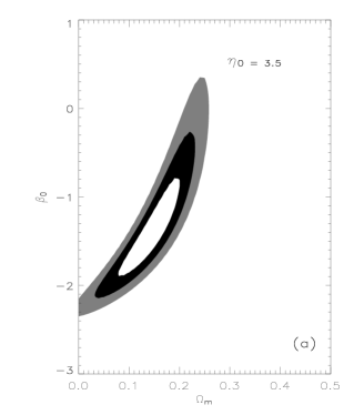
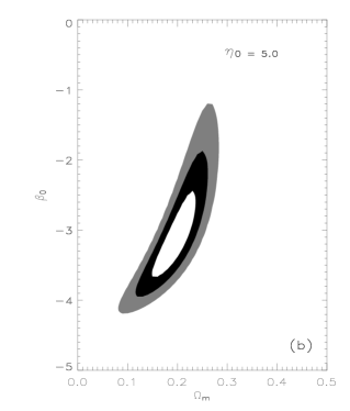
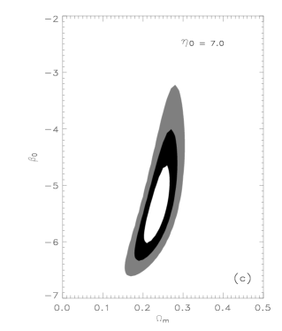
Figure 1: Contours of $\chi^{2}$ in the parametric space $\Omega_{m}-\beta_{0}$. In all panels, the contours are drawn for $\Delta\chi^{2}=2.30$ and $6.17$. As explained in the text, the value of $\eta_{0}$ has been fixed at 3.5 (a), 5.0 (b) and 7.0 (c). In particular, we note that for $\eta_{0}=7.0$, the allowed 1$\sigma$ interval for the matter density parameter is very close to that provided by current dynamical estimates, i.e., $\Omega_{m}\simeq 0.2-0.3$.

In order to study the acceleration phenomenon in these scenarios we use the measured distance-redshift relation of SNe Ia, which provides the most direct probe of the current accelerating expansion. In our analysis we eliminate the contribution of $\Omega_{\Lambda}$ in Eq. (29) to emphasize the relevance of the extrinsic curvature to the accelerated expansion of the universe. Motivated by recent CMB results [28] we also assume $\Omega_{k}=0$ and use the normalization condition $\Omega_{\rm{ext}}=(1-\Omega_{m})/e^{\gamma(0)}$.

In a flat universe, the dimensionless luminosity-distance is written as

$$d_{L}(z)H_{0}=(1+z)\Gamma(z)$$ (30)

where $\Gamma(z)=\int_{0}^{z}{dz^{\prime}/{{E}}(z^{\prime})}$ and the function $E(z^{\prime})$ is given by Eq. (29). In our analysis, we use the SNLS collaboration sample of 115 SNe Ia published by Astier et al. in Ref. [29] (for more details on SNe Ia statistical analysis we refer the reader to [30, 31, 32, 33, 34, 36, 35] and Refs. therein).

Figure (1a)-(1c) show the results of our statistical analysis. Contours of constant $\Delta\chi^{2}=2.30$, 6.17 and 11.8 are displayed in the $\Omega_{m}-\beta_{0}$ space for three different values of $\eta_{0}$. Since the highest-$z$ SNe Ia in our sample is at $z\simeq 1.01$, we note that the constraint (28) implies $\eta_{0}\geq 3.5$, which is the first value considered. The other two values, i.e., $\eta_{0}=5.0$ and $\eta_{0}=7.0$ are taken arbitrarily. At 68.3% (C.L.), we have found for $\eta_{0}$ = 3.5, 5.0 and 7.0, respectively,

$$\beta_{0}=-1.45^{+0.30}_{-0.25}\quad\mbox{and}\quad\Omega_{m}=0.14\pm 0.03\;,$$

$$\beta_{0}=-3.09^{+0.5}_{-0.4}\quad\mbox{and}\quad\Omega_{m}=0.20\pm 0.03\;,$$

and

$$\beta_{0}=-5.35^{+0.7}_{-0.6}\quad\mbox{and}\quad\Omega_{m}=0.24\pm 0.03\;.$$

By combining the above results with the normalization condition $\Omega_{\rm{ext}}=(1-\Omega_{m})/e^{\gamma(0)}$ obtained from Eq. (29), we estimate the extrinsic curvature density parameter to lie in the interval $10^{-2}\lesssim\Omega_{\rm{ext}}\lesssim 10^{-6}$.

5 Final Remarks

The four-dimensionality of space-times is a consequence of the well established experimental structure of special relativity, particle physics and quantum field theory, using only the observables which interact with the standard gauge fields and their dual properties. This has been described as confined quantities, and it includes all observations that are made through gauge interactions. Any other observed effects, usually labeled as ”dark”, are known only through their gravitational consequences. Therefore, it is possible that the such ”darkness” is associated with the fact that the gravitational field is not a gauge field, and consequently it is not necessarily confined. The only known property of Riemannian geometry describing the perturbations of geometry along the extra dimensions is Nash’s theorem on local and differentiable perturbative embedded Riemannian manifolds.

In this paper we have described the current cosmic acceleration as a consequence of the extrinsic curvature of the FLRW universe, locally embedded in a 5-dimensional space defined by the Einstein-Hilbert action. As discussed in Sec. III, Nash’s theorem uses the extrinsic curvature as field which provides the propagation of the gravitational field along the extra dimensions. However, as a consequence of the four-dimensional confinement of gauge fields and ordinary matter, the extrinsic curvature is not completely determined by the embedding equations. Therefore, in order to complement the number of required equations, we have noted that the extrinsic curvature is a rank-2 symmetric tensor, which corresponds to a spin-2 field defined on the embedded space-time. As it was demonstrated by Gupta, any spin-2 field satisfies an Einstein-like equation. After the due adaption to an embedded space-time, we have constructed the Gupta equations for the extrinsic curvature of the FLWR geometry and studied the behavior of its solution at the current stage of the cosmic evolution. We have also tested the observational viability of these scenarios by confronting their theoretical predictions for an accelerating universe with current SNe Ia data. We have shown that a very small contribution of $\Omega_{\rm{ext}}$ ($\sim 10^{-2}-10^{-6}$) is enough to provide a possible explanation for the current observed accelerated expansion of the Universe.

References

- [1] B. Carter and J. P. Uzan, Nucl. Phys. B606, 45 (2001).
- [2] N. Arkani-Hamed et al., Phys. Lett. B429, 263 (1998).
- [3] L. Randall and R. Sundrum, Phys. Rev. Lett. 83, 3370,(1999).
- [4] L. Randall and R. Sundrum, Phys. Rev. Lett. 83, 4690 (1999).
- [5] G. Dvali, G. Gabadadze and M. Porrati, Phys. Lett. B485, 208 (2000)
- [6] V. Sahni and Y. Shtanov, IJMP D11, 1515 (2002).
- [7] V. Sahni and Y. Shtanov, JCAP 0311, 014 (2003).
- [8] T. Shiromizu, K. Maeda, and M. Sasaki, Phys. Rev. D62, 024012 (2000).
- [9] R. Dick, Class. Quantum Grav. 18, R1 (2001).
- [10] C. J. Hogan, Class. Quant. Grav. 18, 4039 (2001).
- [11] C. Deffayet, G. Dvali and G. Gabadadze, Phys. Rev. D65, 044023 (2002).
- [12] J. S. Alcaniz, Phys. Rev. D 65, 123514 (2002).
- [13] D. Jain, A. Dev and J. S. Alcaniz, Phys. Rev. D66, 083511 (2002).
- [14] A. Lue, Phys. Rept. 423, 1 (2006).
- [15] M. Heydari-Fard, M. Shirazi, S. Jalalzadeh and H. R. Sepangi, Phys. Lett. B 640, 1 (2006).
- [16] M. D. Maia, E. M. Monte, J. M. F. Maia and J. S. Alcaniz, Class. Quant. Grav. 22, 1623 (2005).
- [17] M. D. Maia, E. M. Monte and J. M. F. Maia, Phys. Lett. B585, 11 (2004).
- [18] W. Pauli, and M. Fierz. Proc. R. Soc. Lond. A173, 211, (1939).
- [19] S. N. Gupta, Phys. Rev. 96, (6) (1954).
- [20] C. Fronsdal, Phys. Rev. D18 3624 (1978).
- [21] C. J. Isham, A. Salam and J. Strathdee. Phys. Rev. 3, 4 (1971).
- [22] P. J. McCarthy, Proc. Royal Soc. London. A 330, 517 (1972).
- [23] M. D. Maia, A. J. S. Capistrano, E. M. Monte, Int. J. Mod. Physics A 24, 1545 (2009).
- [24] J. Nash, Ann. Maths. 63, 20 (1956)
- [25] M. D. Maia, N. Silva and, M. C. B. Fernandes, JHEP 047, 0704 (2007).
- [26] W. Pauli, and M. Fierz. Proc. R. Soc. Lond. A173, 211, (1939).
- [27] S. N. Gupta, Phys. Rev. 96, (6) (1954).
- [28] D. N. Spergel et al., Astrophys. J. Supl. 170, 377 (2007).
- [29] P. Astier et al., Astron. Astrophys. 447, 31 (2006).
- [30] T. Padmanabhan and T. R. Choudhury, Mon. Not. R. Astron. Soc. 344, 823 (2003).
- [31] P. T. Silva and O. Bertolami, Astrophys. J. 599, 829 (2003).
- [32] Z. H. Zhu and J. S. Alcaniz, Astrophys. J. 620, 7 (2005).
- [33] J. S. Alcaniz, Phys. Rev. D 69, 083521 (2004).
- [34] T. R. Choudhury and T. Padmanabhan, Astron. Astrophys. 429, 807 (2005).
- [35] L. Samushia and B. Ratra, Astrophys. J. 650, L5 (2006).
- [36] M. Kowalski et al., Astrophys. J. 686, 749 (2008).