Bifurcation and chaos in zero Prandtl number convection

Abstract

We present the detailed bifurcation structure and associated flow patterns near the onset of zero Prandtl number Rayleigh Bénard convection. We employ both direct numerical simulation and a low-dimensional model ensuring qualitative agreement between the two. Various flow patterns originate from a stationary square observed at a higher Rayleigh number through a series of bifurcations starting from a pitchfork followed by a Hopf and finally a homoclinic bifurcation as the Rayleigh number is reduced to the critical value. Global chaos, intermittency, and crises are observed near the onset.

Thermal convection is observed almost everywhere in the universe: industrial appliances, liquid metals, atmosphere, oceans, interiors of planets and stars, galaxies etc. An idealized version of convection called Rayleigh Bénard convection (RBC) has been studied for almost a century and it is still an area of intense research rbc_etc . The two most important parameters characterizing convection in RBC are the Rayleigh number, describing the vigour of buoyancy, and the Prandtl number, being the ratio of kinetic viscosity and thermal diffusivity. Solar solar and geological flows geo are considered to have very low Prandtl numbers, as do flows of liquid metals metal . RBC exhibits a wide range of phenomena including instabilities, patterns, chaos, spatio-temporal chaos, and turbulence for different ranges of Rayleigh number and Prandtl number rbc_etc . Origin of instabilities, chaos, and turbulence in convection is one of the major research topics of convection.

Direct numerical simulation (DNS), due to its high dimensionality, generates realistic but excessively voluminous numerical outputs which obscure the underlying dynamics. Lower dimensional projections lead to models which, if done improperly, lose the overall physics. In this letter, our aim is to unfold and discover the underlying physics of low Prandtl number flows lowp by examining the natural limit of zero Prandtl number (zero-P) thual ; spiegel ; kumar1 ; busse ; herring ; knobloch ; pal . This offers a dramatic simplification without sacrificing significant physics, as well as displays a fascinatingly rich dynamic behaviour. In particular, since zero-P flows are chaotic immediately upon initiation of convection, we adopt a nonstandard strategy of approaching this system from the post-bifurcation direction. Moreover, we attack the problem simultaneously with DNS (to ensure accuracy) as well as a low dimensional model (to aid physical interpretation); and we stringently refine both the model and DNS until satisfactory agreement is obtained at all levels of observed behaviour. Our results show a diverse variety of both new and previously observed flow patterns. These flow patterns emerge as a consequence of various bifurcations ranging from pitchfork, Hopf and homoclinic bifurcations to bifurcations involving double zero eigenvalues.

Convection in an arbitrary geometry is quite complex, so researchers have focused on convective flow between two conducting parallel plates called Rayleigh Bénard convection rbc_etc . The fluid has kinematic viscosity $\nu$, thermal diffusivity $\kappa$, and coefficient of volume expansion $\alpha$. The top and bottom plates are separated by distance $d$ and are maintained at temperatures $T_{1}$ and $T_{2}$ respectively with $T_{1}>T_{2}$. Convective flow in RBC is characterized by the Rayleigh number $R=\alpha(T_{1}-T_{2})gd^{3}/\nu\kappa$, where $g$ is the acceleration due to gravity, and the Prandtl number $P=\nu/\kappa$. Various instabilities, patterns, and chaos, are observed for different ranges of $R$ and $P$ rbc_etc ; thual ; pattern . Transition to chaotic states through various routes have been observed in convection expt ; dns .

In this letter, we focus on zero-P convection. The governing zero-P Boussinesq equations spiegel are nondimensionalized using $d$ as length scale, $d^{2}/\nu$ as time scale, and $\nu(T_{1}-T_{2})/\kappa$ temperature scale which yields

$$\partial_{t}(\nabla^{2}v_{3}) = \nabla^{4}v_{3}+R\nabla^{2}_{H}\theta$$ (1)

$$-\hat{\bf e}_{3}\cdot\nabla\times\left[(\mbox{\boldmath$\omega$}{\cdot}\nabla){\bf v}-({\bf v}{\cdot}\nabla)\mbox{\boldmath$\omega$}\right],$$

$$\partial_{t}\omega_{3} = \nabla^{2}\omega_{3}+\left[(\mbox{\boldmath$\omega$}{\cdot}\nabla)v_{3}-({\bf v}{\cdot}\nabla)\omega_{3}\right],$$ (2)

$${\nabla}^{2}\theta = -v_{3},$$ (3)

$$\nabla{\cdot}{\bf v} = 0,$$ (4)

where ${\bf v}\equiv(v_{1},v_{2},v_{3})$ is the velocity field, $\theta$ is the deviation in the temperature field from the steady conduction profile, $\mbox{\boldmath$\omega$}=\nabla\times{\bf v}$ is the vorticity field, $\hat{\bf e}_{3}$ is vertically directed unit vector, and $\nabla_{H}^{2}=\partial_{xx}+\partial_{yy}$ is the horizontal Laplacian. We consider perfectly conducting and free-slip boundary conditions at the top and bottom plates, and periodic boundary conditions along horizontal directions thual ; dns . In the following discussion we also use the reduced Rayleigh number $r=R/R_{c}$ where $R_{c}$ is the critical Rayleigh number.

Straight two-dimensional (2D) rolls that have zero vorticity are neutrally stable solution of zero-P convection at $r=1$. However they become unstable for $r>1$. Busse busse , Thual thual and Kumar et. al. kumar1 showed that these 2D rolls saturate through generation of vorticity (wavy rolls) for $r>1$ both for low Prandtl number and zero-P fluids. Thus vorticity plays a critical role in zero-P convection.

Herring herring was first to simulate these equations under free-slip boundary conditions. However he observed divergence of the solutions possibly due to the instabilities described above. The first successful simulation of zero-P equations with free-slip boundary conditions was done by Thual thual . He reported many interesting flow patterns including relaxation oscillation of square patterns (SQOR) and stationary square patterns (SQ). Later Knobloch knobloch explained the stability of the SQ patterns using the amplitude equations. Pal and Kumar pal explained the mechanism of selection of square patterns using a 15-dimensional model. Note that asymmetric squares (referred to as ‘cross roll’ in literature) and other patterns have been observed in experiments of low-Prantl number convection expt_pattern ; rbc_etc .

We performed around 100 DNS runs of zero-P convection (Eqs. (1-4)) using a pseudo-spectral code for various $r$ values on $64^{3}$ box. The aspect ratio of our simulation is $2\sqrt{2}:2\sqrt{2}:1$. In DNS we observe stationary squares (SQ), stationary asymmetric squares (ASQ), oscillatory asymmetric squares (OASQ), relaxation oscillations with squares (SQOR), and chaos.

For our bifurcation analysis we construct a low-dimensional model using the energetic modes of the above-mentioned simulation in the range of $r=1-1.4$. We pick 9 large-scale vertical velocity modes (real Fourier amplitudes): $W_{101}$, $W_{011}$, $W_{202}$, $W_{022}$, $W_{103}$, $W_{013}$, $W_{112}$, $W_{121}$, $W_{211}$, and 4 large-scale vertical vorticity modes (real Fourier amplitudes): $Z_{110}$, $Z_{112}$, $Z_{121}$, $Z_{211}$. The three subscripts are the indices of wavenumber along x,y, and z directions. Cumulative energy contained in these modes ranges from 85% to 98% of the total energy of DNS, and each of these modes has 1% or more of the total energy. We derive the model equations by the Galerkin projection of Eqs. (1-4) on the subspace of these modes. This results in thirteen coupled first-order ordinary differential equations for the above variables. The low-dimensional model captures all the flow patterns of DNS mentioned above. The range of $r$ for these patterns for the model and DNS are shown in Table 1, and they are reasonably close to each other. Interestingly, the stable steady values of the modes $W_{101}$, $W_{011}$, $W_{112}$, $W_{121}$, $W_{211}$ for SQ and ASQ patterns match with corresponding DNS values within 10%.

Flow patterns	r (Model)	r (DNS)
Chaotic	1 - 1.0045	1 - 1.0048
SQOR	1.0045 - 1.0175	1.0048 - 1.0708
OASQ	1.0175 - 1.0703	1.0709 - 1.1315
ASQ	1.0703 - 1.2201	1.1316 - 1.2005
SQ	1.2201 - 1.4373	1.2006 - 1.4297

Table 1: Range of reduced Rayleigh number $r$ corresponding to various flow patterns observed in the model and the DNS. Here SQ, ASQ, OASQ, and SQOR represent stationary squares, stationary asymmetric squares, oscillatory asymmetric squares, and relaxation oscillation of squares respectively.

The origin of the above flow patterns can be nicely understood using the bifurcation diagram of the low-dimensional model. To generate the bifurcation diagram, we first evaluate a fixed point numerically using Newton-Raphson method for a given $r$. The branch of fixed points is subsequently obtained using a fixed arc-length based continuation scheme wahi . Stability of the fixed points is ascertained through an eigenvalue analysis of the Jacobian and accordingly the bifurcation points are located. New branches of fixed points are born when the eigenvalue(s) become zero (pitchfork), and branches of periodic solutions appear when the eigenvalue(s) become purely imaginary (Hopf). Subsequent branches are generated by calculating and continuing the new steady solutions close to the bifurcation points.

Fixed points are the backbone of bifurcation diagram. For $r<1$, the origin is the unique stable fixed point corresponding to the pure conduction state. There is a double zero eigenvalue at $r=1$ Guck_Holmes , and all the fixed points (13 in number) arising from $r=1$ are unstable for $r>1$. These fixed points are shown as dotted lines in Fig. 1. Four of these branches of fixed points bifurcate from the origin; these fixed points satisfy $|W_{101}|=|W_{011}|$. The other 8 branches of unstable fixed points emerge from nonzero $W_{101}$ or $W_{011}$, and they obey $|W_{101}|\neq|W_{011}|$ (see Fig. 1). With an increase of $r$, these 8 branches become stable and merge with the 4 branches that originate from the origin. In Fig. 1, modes $W_{101}$ and $W_{011}$ are presented even though all other modes are also nonzero.

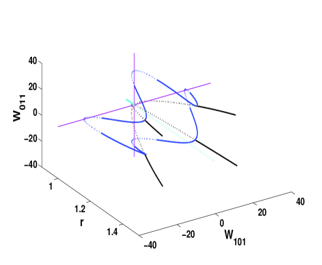
Figure 1: Three dimensional view of the bifurcation diagram showing the fixed points with solid and dashed curves representing the stable and unstable fixed points respectively. Black, blue, and cyan curves represent stationary squares (SQ), asymmetric stationary squares (ASQ), and conduction state respectively. All the points on the axis (purple lines) are 2D roll solutions.

After a discussion on fixed points, we focus on the complete bifurcation diagram shown in Fig. 2. Chaotic solutions are observed at the onset of convection itself, i.e., just above $r=1$. A better insight into the origin of the various solutions is facilitated by starting the analysis at a higher $r$ value and tracking the various bifurcations while approaching $r=1$.

Figure 2: Bifurcation diagram of the model for $0.95\leq r\leq 1.4$. The stable branches corresponding to stationary squares (SQ) and stationary asymmetric squares (ASQ) are represented by solid black and solid blue lines respectively. Red, green, and brown curves represent the extrema of oscillatory asymmetric squares (OASQ), relaxation oscillation of squares (SQOR), and chaotic solutions respectively. A zoomed view of the bifurcation diagram for the chaotic regime is shown in the inset. Branches corresponding to the unstable fixed points are represented by dashed lines. Cyan line represents the conduction state.

We start our analysis at $r=1.4$ where we observe stable symmetric squares (SQ) with $|W_{101}|=|W_{011}|$ (black curve in Fig. 1). In Fig. 2 we represent only the $W_{101}=W_{011}$ solution. As $r$ is reduced from $1.4$, the SQ branch of fixed points loses stability via a supercritical pitchfork bifurcation at $r\approx 1.2201$, after which we observe stationary solutions with $W_{101}\neq W_{011}$ (blue curves of Figs. 1 and 2). These solutions correspond to asymmetric square patterns (ASQ), either dominant along x axis ($|W_{101}|>|W_{011}|$), or dominant along y axis ($|W_{101}|<|W_{011}|$). The SQ solution $|W_{101}|=|W_{011}|$ continues as a saddle. With a further reduction of $r$, ASQ branches lose stability through a supercritical Hopf bifurcation at $r\approx 1.0703$ and limit cycles are born. These limit cycles are represented by red curves in Fig. 2. Physically they represent oscillatory asymmetric square patterns (OASQ). Fig. 3(a) illustrates the projection of two of these stable limit cycles (for $r=1.0494$) on the $W_{101}-W_{011}$ plane.

Figure 3: Phase space projections of limit cycles on the $W_{101}-W_{011}$ plane for (a) $r=1.0494$ and (b) $r=1.0099$. The limit cycles in figure (a) merge to form a single limit cycle in figure (b). Black dots indicate the symmetric square saddle.

The limit cycles grow in size as $r$ is lowered. A homoclinic orbit is formed at $r\approx 1.0175$. Afterwards, homoclinic chaos is observed in a narrow window. At lower $r$ the attractor becomes regular resulting in a larger limit cycle that corresponds to the relaxation oscillations with an intermediate square pattern (SQOR). Fig. 3($b$) illustrates the projection of this limit cycle at $r=1.0099$. The flow pattern in this regime changes from an approximate pure roll in one direction to a symmetric square, and then to an approximate pure roll in the perpendicular direction. The SQOR solution is represented by the green curve in Fig. 2.

The flow becomes chaotic as $r\rightarrow 1$. The chaotic flow manifests itself in three different forms: Ch1, Ch2, and Ch3 as shown in the inset of Fig. 2 as (i), (ii), and (iii) respectively. The phase space projection for these three solutions are depicted in Fig. 4 for $r=1.0041$, 1.0038 and 1.0030 for the 13-mode model, and for $r=1.0045$, 1.0032 and 1.0023 in the DNS. Their chaotic nature is confirmed by the positivity of the largest Lyapunov exponent (0.0131, 0.0254 and 0.0389) calculated using the 13-mode model for $r=1.0041$, 1.0038 and 1.0030 respectively.

Figure 4: The three different chaotic solutions observed near $r=1$: Ch1 at $r=1.0041$ for the model (a) and at $r=1.0045$ in DNS (b); Ch2 at $r=1.0038$ for the model (c) and at $r=1.0030$ in DNS (d); Ch3 at $r=1.0030$ for the model (e) and at $r=1.0023$ in DNS (f). These solutions belong to (i), (ii), and (iii) regimes in the bifurcation diagram (Fig. 2).

The first chaotic solution, Ch1 (Figs. 4(a) and 4(b)) results from the broadening of the limit cycle attractor with chaotic switchings between the two lobes of the attractor. This global chaos could probably be attributed to homoclinic tangles. The time-series of the solution shows intermittency. At $r\approx 1.004$, these four chaotic attractors of Ch1 merge in a ‘crisis’ to yield a single large chaotic attractor Ch2 (Figs. 4(c) and 4(d)). This chaotic solution persists till $r\approx 1.0035$ after which it splits into four different chaotic attractors Ch3 in another ‘crisis’, one of which is shown in Figs. 4(e) and 4(f). The time-series again shows intermittency, and the flow pattern switches from an approximately pure roll in one direction to an asymmetric square. With a further reduction in the Rayleigh number, the size of these chaotic attractors decreases and they ultimately merge with one of the branches of the unstable ASQ fixed points at $r=1$. In Fig. 2, we exhibit the merger of one of these chaotic attractors with the unstable ASQ fixed point with $W_{101}\rightarrow 0$.

In conclusion, we present for the first time a numerically obtained, DNS validated, detailed bifurcation diagram and associated flow structures of zero-P convective flow near the onset of convection. The whole spectrum of phenomena observed in DNS near the onset of convection is replicated by the low-dimensional model. Hence, the bifurcation structure presented here explains the origin and dynamics of various patterns near the onset of convection. Recent analysis of VKS (Von-Karman-Sodium) experimental results indicate a strong role of large-scale modes for the magnetic field reversal VKS . A study of large-scale modes as outlined in this letter may provide useful insights into the mechanism behind the generation and reversal of magnetic field. The dynamics of large-scale modes in other hydrodynamic systems like rotating turbulence, magneto-convection etc. could also be captured by a similar approach.

A careful analysis of DNS results indicate the existence of fringe attractors apart from the main attractors presented in this letter. These new attractors are relatively insignificant and they exist only in localized regimes of $r$. A detailed investigation of all the attractors will be reported elsewhere. Bifurcation analysis for $r>1.4$ is reasonably complex as well. Also preliminary results show a reasonable amount of similarity between low Prandtl number convection and zero-P convection. These issues are under investigation.

We thank S. Fauve, A. Chatterjee, A. K. Mallik, and V. Subrahmanyam for useful discussions. We thank Computational Research Laboratory, India for providing us access to the supercomputer EKA where part of this work was done. This work was supported by the research grant of Department of Science and Technology, India.

References

- (1) S. Chandrasekhar, Hydrodynamic and Hydromagnetic Stability (Cambridge University Press, Cambridge, 1961); F. H. Busse, in Hydrodynamic Instabilities and the Transition to Turbulence, edited by H. L. Swinney and J. P. Gollub, Topics in Appl. Phys., 45 (Springer, Berlin, 1985), pp. 97 - 137; P. Manneville, Instabilities, Chaos and Turbulence, (Imperial College Press, London, 2004); G. Ahlers, S. Grossmann, and D. Lohse, Rev. Mod. Phys 81, 503 (2009).
- (2) R. F. Stein and A. Norlund, Solar Physics 192, 91 (2000); F. Cattaneo, T. Emonet, and N. Weiss, Astrophysical J. 588, 1183 (2003).
- (3) F. H. Busse, in Fundamentals of thermal convection,Mantle Convection, Plate tectonics and Global Dynamics, edited by W. R. Peltier, (Gordon and Breach, 1989), pp 23-95.
- (4) P. A. Davidson, An Introduction to Magnetohydrodynamics, (Cambridge University Press, Cambridge, 2001).
- (5) M. R. E. Proctor, J. Fluid Mech. 82, 97 (1977); R. M. Clever and F. H. Busse, J. Fluid Mech. 102, 61 (1981); I. G. Kevrekidis et al., Physica D 71, 342 (1994); E. Bodenschatz, W. Pesch, and G. Ahlers, Annu. Rev. Fluid Mech., 32, 709 (2000).
- (6) O. Thual, J. Fluid Mech. 240, 229 (1992).
- (7) E. A. Spiegel, J. Geophys. Res. 67, 3063 (1962).
- (8) K. Kumar, S. Fauve, and O. Thual, J. Phys. II (France) 6, 945 (1996); K. Kumar, Woods Hole Oceanogr. Inst. Tech. Rep. WHOI-90-01, (1990) (unpublished).
- (9) F. H. Busse, J. Fluid Mech. 52, 97 (1972).
- (10) J. R. Herring, Woods Hole Oceanogr. Inst. Tech. Rep. WHOI-70-01, (1970).
- (11) E. Knobloch, J. Phys. II France 2, 995 (1992).
- (12) P. Pal, and K. Kumar, Phys. Rev. E 65, 047302 (2002).
- (13) M. C. Cross and P. C. Hohenberg, Rev. Mod. Phys. 65, 851 (1993); Y. C. Hu, R. Ecke and G. Ahlers, Phys. Rev. Lett. 72, 2191 (1994); J. Liu and G. Ahlers, Phys. Rev. Lett. 77, 3126 (1996); D. A. Egolf et al., Nature 404 733 (2000); K. Kumar, S. Chaudhuri, and A. Das, Phys. Rev. E 65, 026311 (2002).
- (14) J. Maurer and A. Libchaber J. Physique Lett., 41, 515 (1980); P. Berge et al., J. Physique Lett., 41, 341 (1980); J. P. Gollub and S. V. Benson, J. Fluid Mech., 100, 449 (1980); M. Giglio, S. Mussazi and V. Perini, Phys. Rev. Lett., 47, 243 (1981); A. Libchaber, C. Laroche and S. Fauve, J. Physique Lett., 43, 211 (1982).
- (15) M. Meneguzzi et al., J. Fluid Mech. 182, 169 (1987).
- (16) V. Croquette, Contemporary Physics 30, 113 (1989); V. Croquette, Contemporary Physics 30, 153 (1989).
- (17) K. Nandakumar, and A. Chatterjee, Nonlin. Dynam. 40, 143 (2005); P. Wahi, and A. Chatterjee, Int. J. Nonlin. Mech. 43(2), 111 (2008).
- (18) J. Guckenheimer and P. Holmes, Nonlinear Oscillations, Dynamical Systems, and Bifurcations of Vector Fields (New York, Springer, 1983).
- (19) F. Pétrélis et al., Phys. Rev. Lett. 102, 144503 (2009).