A POSSIBLE CONNECTION BETWEEN
MASSIVE FERMIONS AND DARK ENERGY

Abstract

In a dense cloud of massive fermions interacting by exchange of a light scalar field, the effective mass of the fermion can become negligibly small. As the cloud expands, the effective mass and the total energy density eventually increase with decreasing density. In this regime, the pressure-density relation can approximate that required for dark energy. We apply this phenomenon to the expansion of the Universe with a very light scalar field and infer relations between the parameters available and cosmological observations. Majorana neutrinos at a mass that may have been recently determined, and fermions such as the Lightest Supersymmetric Particle (LSP) may both be consistent with current observations of dark energy.

I Introduction

Several years ago it was suggested that neutrinos might interact weakly among themselves through the exchange of a very light scalar particle MKY ; TRE , with possible consequences for the evolution of the Universe and for the propagation of neutrinos from distant events. We examined such a system for scalars with astrophysical ranges to explore the possibility of neutrino clustering SGM and noted at the time that the neutrino clouds thus formed could seed structure formation in the Early Universe. More generally, in such clouds of massive fermions interacting by exchange of a light scalar field, the effective mass of the fermion can become negligibly small. We found that, as a consequence, when the cloud expands, the effective mass and the total energy density must eventually increase with decreasing density. We studied this system in 1996 SGM , well before the discovery of Dark Energy, in connection with experimental problems encountered in the search for the mass of the (electron) neutrino. Those anomalies have since disappeared, but provided us with the technology to describe dark energy in a well understood dynamical system.

In the following, we first review our previous work on the theory of massive fermions interacting via exchange of a scalar field. This is carried out with scaled variables so the regime of applicability is not constrained. We next recall the relation between Dark Energy and equations of state and define the $w$ parameter used therein. After this, we apply our model results for $w$ and discuss the numerical, analytical and scaling properties relevant to the accuracy of our results. Penultimately, we extract a rough mass value from applying those results to describe Dark Energy assuming the currently accepted value for its energy density in the epoch corresponding to $z=1$. Finally, we present our conclusions and discuss some open questions.

II Summary of a Theory of Massive Fermions
Interacting via Light Scalar Field Exchange

The effective Lagrangian for a Dirac field, $\psi$, interacting with a scalar field, $\phi$, is:

$${\cal L}=\bar{\psi}(i/\!\!\!\partial-m_{\nu}^{(0)})\psi+{\scriptsize\frac{1}{2}}\left[\phi(\partial^{2}-m_{s}^{2})\phi\right]+g\bar{\psi}\psi\phi$$ (1)

which gives as the equations of motion

$$\left[\partial^{2}+m_{s}^{2}\right]\phi = g\bar{\psi}\psi$$ (2)

$$\left[i/\!\!\!\partial-m_{\nu}^{(0)}\right]\psi = -g\phi\psi.$$ (3)

As usual, we set $\bar{h}=c=1$. We have omitted nonlinear scalar selfcouplings here, even though they are required to exist by field theoretic selfconsistency, MGGS as they may consistently be assumed to be sufficiently weak as to be totally irrelevant. The parameter $m^{(0)}_{f}$ is the renormalized vacuum mass that the fermion would have in isolation, and takes into account any contributions from all other interactions, as well as contributions from the vacuum expectation value of the new scalar field, $\phi$.

We look for solutions of these equations in infinite matter which are static and translationally invariant. Eq.(2) then gives

$$\phi=\frac{g}{m_{s}^{2}}\bar{\psi}\psi,$$ (4)

which, when substituted in Eq.(3) gives an effective mass for the fermion of

$$m^{*}_{f}=m^{(0)}_{f}-\frac{g^{2}}{m_{s}^{2}}\bar{\psi}\psi.$$ (5)

These equations are operator equations. We next act with each of these equations on a state $|\Omega\rangle$ defined as a filled Fermi sea, with a number density $n$ per fermion state, and Fermi momentum $k_{F}$, related as usual by $n~{}=~{}{k_{F}}^{3}/(6\pi^{2})$. The operator $\bar{\psi}\psi$ acting on this state gives

$$\bar{\psi}\psi|\Omega\rangle=\frac{\zeta}{(2\pi)^{3}}\int_{|\vec{k}|<k_{F}}d^{3}k\left|\frac{m^{*}_{f}}{\sqrt{(m^{*}_{f})^{2}+k^{2}}}\right||\Omega\rangle,$$ (6)

where $\zeta$ is the number of fermion states which contribute — $\zeta~{}=~{}2$ for Majorana fermions and $\zeta~{}=~{}4$ for Dirac fermions. Thus the effective mass is determined by an integral equation

$$m^{*}_{f}=m^{(0)}_{f}-\frac{g^{2}\zeta}{2\pi^{2}m_{s}^{2}}\int_{0}^{k_{F}}k^{2}\,dk\frac{m^{*}_{f}}{\sqrt{(m^{*}_{f})^{2}+k^{2}}.}$$ (7)

To discuss the solutions of this equation, we reduce it to dimensionless form, dividing by $m^{(0)}_{f}$, and introducing the parameter

$$K_{0}~{}\equiv~{}\zeta\frac{g^{2}(m^{(0)}_{f})^{2}}{2\pi^{2}m_{s}^{2}},$$ (8)

and the variables $y~{}=~{}\frac{m^{*}_{f}}{m^{(0)}_{f}},x~{}=~{}\frac{k}{m^{(0)}_{f}},x_{F}~{}=~{}\frac{k_{F}}{m^{(0)}_{f}}$. Then Eq.(7) becomes

$$y = 1-yK_{0}\int_{0}^{x_{F}}\frac{x^{2}\,dx}{\sqrt{y^{2}+x^{2}}}$$ (9)

$$= 1-\frac{yK_{0}}{2}\left[e_{F}x_{F}-y^{2}\ln\left(\frac{e_{F}+x_{F}}{y}\right)\right],$$ (10)

with $e_{F}~{}\equiv~{}\sqrt{x_{F}^{2}+y^{2}}$. This choice of scaled variables gives all energies (and momenta) in units of the vacuum fermion mass. For consistency, we define the dimensionless scalar mass as $\mu=\frac{m_{s}}{m^{(0)}_{f}}$ in these same units. One can regard Eq.(10) as a non-linear equation for $y$ as a function of either $e_{F}$ or $x_{F}$. As a function of $e_{F}$, $y$ is multiple valued (when a solution exists at all), whereas $y$ is a single valued function of $x_{F}$.

The total energy of the system is a sum of the energy of the fermions, $E_{f}~{}=~{}e_{f}~{}m^{(0)}_{f}~{}\zeta N$, and the energy in the scalar field, $E_{s}~{}=~{}e_{s}~{}m^{(0)}_{f}~{}\zeta N$, where $N$ is the total number of neutrinos in each contributing state. These expressions serve to define the per fermion quantities $e_{f}$ and $e_{s}$. Also, $E_{s}~{}=~{}{\cal E}_{s}~{}V$, where ${\cal E}_{s}~{}=~{}\frac{1}{2}m_{s}^{2}\phi^{2}$ is the energy density of the (here uniform) scalar field.

One finds that

$$e_{f} = \frac{3}{x_{F}^{3}}\int_{0}^{x_{F}}x^{2}\,dx\sqrt{x^{2}+y^{2}}$$ (11)

$$= \frac{3}{x_{F}^{3}}\left\{\frac{e_{F}x_{F}^{3}}{4}+\frac{e_{F}x_{F}y^{2}}{8}-\frac{y^{4}}{8}\ln\left(\frac{e_{F}+x_{F}}{y}\right)\right\}$$

and

$$e_{s} = \frac{K_{0}}{2}\frac{3}{x_{F}^{3}}y^{2}\left(\int_{0}^{x_{F}}\frac{x^{2}\,dx}{\sqrt{x^{2}+y^{2}}}\right)^{2}$$ (12)

$$= \frac{1}{2K_{0}}\frac{3}{x_{F}^{3}}(1-y)^{2}.$$

and the total energy density per fermion is just the sum,

$$<e>=e_{f}+e_{s}.$$ (13)

Notice that for large values of $x_{F}$,

$$y \rightarrow \frac{2}{K_{0}x_{F}^{2}}$$

$$e_{f} \rightarrow \frac{3e_{F}}{4}$$

$$\rightarrow \frac{3x_{F}}{4}$$

$$e_{s} \rightarrow \frac{3}{2K_{0}}\frac{1}{x_{F}^{3}}.$$ (14)

It is also useful to note that, for small $x_{F}$,

$$y \rightarrow 1-\frac{K_{0}x_{F}^{3}}{3}$$

$$e_{f} \rightarrow 1+\frac{3x_{F}^{2}}{10}$$

$$e_{s} \rightarrow \frac{K_{0}}{2}\frac{x_{F}^{3}}{3}.$$ (15)

For the fermion system to be bound, the minimum of $e~{}=~{}e_{f}~{}+~{}e_{s}$ as a function of density (or $x_{F}$) must be less than 1, its value in the zero density limit. Fig.(1) shows the variation of $e$ and $y$ as a function of $x_{F}$ for several values of $K_{0}$. Note that for sufficiently large $K_{0}$, there is a minimum relative to both the large and small $x_{F}$ regimes, that is, relative to regions of both large and small fermion density.

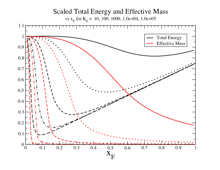
Figure 1: Total energy density per fermion $e$ and effective mass $y$ vs. $x_{F}$ for several values of $K_{0}$.

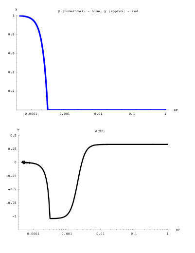
Figure 2: $y$ and $w$ vs. log($x_{F}$) for $K_{0}=10^{11}$.

Thinking of this in terms of expansion of the Universe, early times correspond to the large $x_{F}$ region on the right and late times, including presumably the present, are to the left. Thus we see that at some intermediate period, the energy density passes through a minimum and as the system approaches the present, it passes through a regime in which the energy density is increasing as the number density decreases – characteristic of a regime of negative pressure. Fig.(2) gives an advance peek at the value of the equation of state parameter, $w$, that we derive from the dependence of $e$ vs. $x_{F}$. We will demonstrate later how we do this numerically, but it should be noted that there are still some numerical difficulties evidenced by the ”hash” in the low $x_{F}$ limit where we know that $w\rightarrow 0$ as the cold, now non-interacting fermion ”dust” turns effectively into new ”dark matter”.

III Einstein, FRW and Equations of State

In a Friedmann-LeMaître-Robertson-Walker Universe, Einstein’s equations produce the second order time derivatiive equation of motion that relates the expansion (size) scale parameter, $a$, to Newton’s constant, $G$, the matter density, $\rho$, pressure, $P$, and a cosmological constant, $\Lambda$:

$$\frac{\ddot{a}}{a}=-\frac{4\pi G}{3}(\rho+3P)+\frac{\Lambda}{3}$$ (16)

Therefore, it is necessary to know the relevant equation of state (EoS) before the time development of the scale factor can be determined. For dust, which has no pressure, $P=0$, while for a relativistic gas, $P=\frac{1}{3}\rho$. Note that acceleration of the expansion parameter occurs, even in the absence of a cosmological constant, when $P<-\frac{1}{3}\rho$. Finally, for a spatially and temporally homogenous scalar field, $P<-\rho$, which is more than enough to produce acceleration of the expansion. More generally, we can parametrize equations of state in this regime by a constant, $w$, as

$$P=w\rho$$ (17)

There are a great number of models for this Dark Energy phenomenon. They go by names such as ”quintessence” for $-1<w<0$, or ”phantom energy” for $w<-1$. Among others, this issue has been addressed by Fardon, Nelson and Weiner FNW , Peccei roberto , Barshay and Kreyerhoff BKmpla , Baushev BarX and Mukhopadhyay, Ray and Choudhoury MRC .

III.1 Our EoS

For the system under consideration, the total (matter plus field) energy is given by the product of the total energy density per fermion $<e>$ and the total number of fermions, which in turn is determined by the number density $n$ times the volume, $V$:

$$U=\rho V=m^{(0)}_{f}<e>nV,$$ (18)

where we recall that

$$n=\zeta\frac{(m^{(0)}_{f})^{3}}{6\pi^{2}}x_{F}^{3}$$ (19)

is the fermion number density. The pressure is defined by

$$P=-\frac{\partial U}{\partial V},$$ (20)

where $U$ is the internal energy given above. Since $nV$ is a constant,

$$P = -m^{(0)}_{f}nV\frac{\partial<e>}{\partial V}$$ (21)

$$= -m^{(0)}_{f}nV\frac{\partial n}{\partial V}\frac{\partial<e>}{\partial n}$$

$$= m^{(0)}_{f}n^{2}\frac{\partial<e>}{\partial n}$$

$$= \frac{\rho}{3}\frac{x_{F}}{<e>}\frac{\partial<e>}{\partial x_{F}}$$

$$= \frac{\rho}{3}\frac{\partial ln(<e>)}{\partial ln(x_{F})}$$

From this and Eq.(17), we can identify

$$w=\frac{1}{3}\frac{\partial ln(<e>)}{\partial ln(x_{F})}.$$ (22)

This is our central model result.

IV General Character of Model Results

In Fig.(3), we shows the value of $w$ as computed numerically from Eq.(22) for 8 values of $K_{0}$ on a log scale for $x_{F}<0.4$ and in FIg.(4) for $x_{F}<0.1$ on a linear scale. Note that it approaches close to $-1$ as the density decreases (as the Universe expands and the scale factor $a$ increases from right to left) and then departs sharply towards zero, as also indicated earlier in Fig.(2).

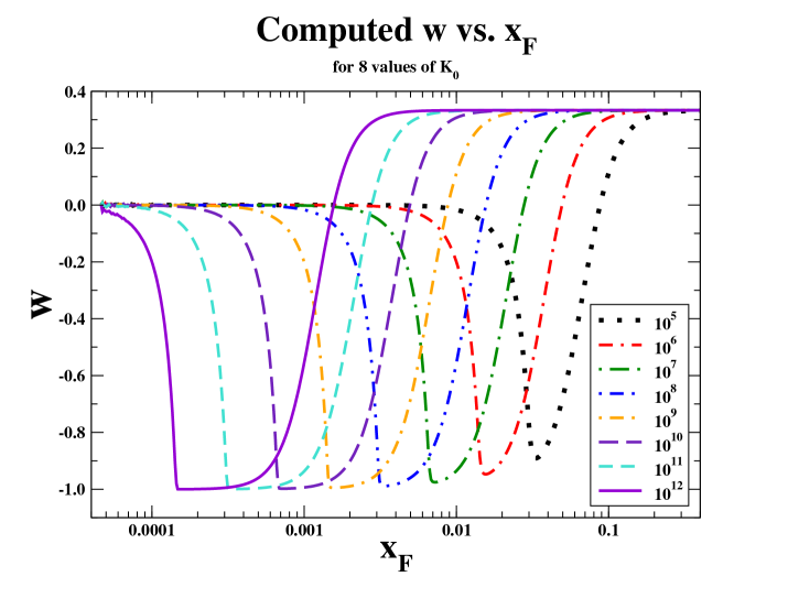
Figure 3: $w$ vs. log($x_{F}$) for 8 values of $K_{0}$.

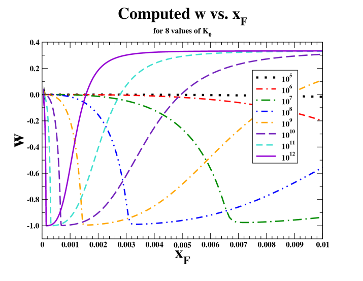
Figure 4: $w$ vs. $x_{F}$ for 8 values of $K_{0}$.

At large $x_{F}$, it is clear that $w$ approaches $+1/3$ as it should for a relativistic gas of fermions. It is perhaps less clear, due to numerical fluctuations, that the value goes to zero at zero density. This can be checked by considering the small $x_{F}$ expansions of the energy densities shown at Eq.(15).

Finally, we performed a number of numerical scaling checks to examine whether $w$ can fall below $-1$. The are shown in Figs.(5,6,7).

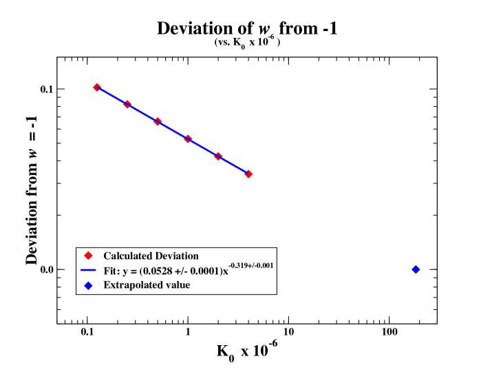
Figure 5: Deviation of minimum value of $w$ from $-1$ vs. $K_{0}$.

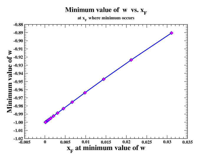
Figure 6: Minimum value of $w$ vs. $x_{F}$ at which minimum occurs, for several values of $K_{0}$.

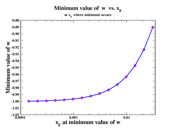
Figure 7: Minimum value of $w$ vs. logarithm of $x_{F}$ at which minimum occurs, for several values of $K_{0}$.

We are continuing our efforts to ensure numerical stability primarily by seeking analytic formulae and approximations, especially to avoid taking derivatives numerically. We will report on these improvements elsewhere, but suffice it to say that we have found no contradiction to the results obtained here by purely numerical means, and confirmed that the difficulties encountered at very small $x_{F}$ are indeed due to numerical noise.

V Numerical Values

All of the above is carried out with scaled variables. However, was shown in Ref.[3], there are only a few, weak constraints on the actual parameter values. Very large values of $K_{0}$ are possible even for very small values of $g^{2}$ if the range of the scalar is very large, corresponding to very small values of $m_{s}$. Even if long-ranged, such weak interactions between fermions, especially neutrinos or those outside of the Standard Model altogether (such as the LSP) are exceptionally difficult to constrain by any laboratory experiments.

The energy density of Dark Energy is quoted density as $(3.20\pm 0.4)\times 10^{-47}\mbox{Gev}^{4}$. In more manageable units, this is given as $(2.3meV)^{4}$. What does this imply for the allowed value of $m_{0}$? If we set this energy density equal to that of this system at $w=-1$,

$$\rho_{\Lambda}=\frac{(m^{(0)}_{f})^{4}<e>x_{F}^{3}}{6\pi^{2}}$$ (23)

then solving for $m^{(0)}_{f}$ gives

$$m^{(0)}_{f}=\{\frac{6\pi^{2}\rho_{\Lambda}}{<e>x_{F}^{3}}\}^{1/4}$$ (24)

If we further suppose that this occurs at cosmological $z\sim 1$, then the range of the scalar field must be comparable to the size of the Universe at that time. That is,

$$m_{s}\sim 7\times 10^{9}\,{\rm lightyears}\sim 3\times 10^{-30}\,{\rm meV}.$$ (25)

For the relatively modest value of $K_{0}\sim 8\times 10^{6}$, this implies that $m^{(0)}_{f}\sim 300{\rm meV}$ and $g^{2}/(4\pi)\sim 6\times 10^{-58}$. These values emphasize the virtual impossibility of constraining this physics by means of laboratory experiments.

We note with interest that following the curve for $y$ from $z=1$ to ”now”, i.e., $z=0$, tells us that the effective mass of this fermion would now be measured to be approximately $(7/8)m^{(0)}_{f}$, a value tantalizingly close to the Majorana neutrino mass that Prof. Klapdor has reported from his experiments Klap .

Other solutions are possible, and Fig.(8) shows how our results scale very accurately (for sufficiently large $K_{0}$) with the 4th root of $K_{0}$, both numerically and under one of our analytic approximations to the region where $w$ is a minimum. In particular, if one has the LSP at $\sim 1$ TeV in mind, $K_{0}$ becomes very large, $\sim 10^{57}$ and $g^{2}/(4\pi)$ also increases, $\sim 10^{-32}$, but these values are not ruled out by anything known.

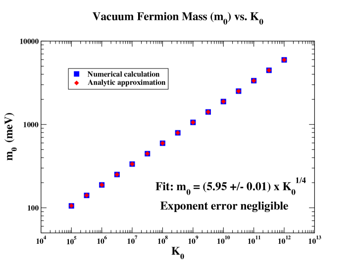
Figure 8: Scaling variation of the vacuum fermion mass, $m^{(0)}_{f}$, vs. $K_{0}$.

VI Conclusions and Questions

We have displayed an explicit and calculable dynamical mechanism that describes Dark Energy and connects it to what in the current epoch becomes a kind of dark matter. Although Dark Matter is usually thought of as existing at early epochs in the life of the Universe, the system described here turns (hot) relativistic fermions, that interact weakly with a very light scalar field, into Dark Energy which lasts for a limited time during the expansion of the Universe which then morphs into new cold dark matter components. Thus, neutrinos can contribute to both. Nor need there be only one time scale or one species for which this applies. (See, e.g., Ref.[12].) If there are many sterile fermions with sufficiently long decay lifetimes, the acceleration/deceleration history of the Universe could be much more complicated that presently envisioned.

We may also ask generally why $w>-1$, but it is fairly clear in this model: A scalar field strength uniform in space and time produces CHT exactly $w=-1$, but here the source for the scalar field is the density of massive fermions. Relativistically, their strength for producing scalar field is severely reduced at high momentum (in the rest frame of the Universe) but as they slow, the scalar field strength grows nonlinearly until, due to the expansion of the Universe, the fermions separate so much (greater than the Yukawa range for exchange of the scalar field) that they cannot act collectively and the scalar field strength declines again.

Finally, we note that our model has definitive if difficult tests, as it predicts specific variations of $w$, slowly approaching $-1$ from above as $z$ decreases through 1, and rising rapidly towards zero as $z$ approaches the present. We hope this encourages observationalists in their efforts to discern variation of $w$ with $z$.

References

- (1) M. Kawasaki, H. Murayama and T. Yanagida, Mod. Phys. Lett. A 7, 563 (1992).
- (2) R. A. Malaney, G. D. Starkman and S. Tremaine, Phys. Rev. D 51, 324 (1995).
- (3) G. J. Stephenson, Jr., T. Goldman and B. H. J. McKellar, Int. J. Mod. Phys. A 13, 2765 (1998); arXiv:hep-ph/9603392.
- (4) B. H. J. McKellar, M. Garbutt, T. Goldman and G. J. Stephenson, Jr., Mod. Phys. Lett. A 19, 1155 (2004).
- (5) J. Dunkley et al., Astrophys. J. Suppl. 180, 306 (2009); arXiv:0803.0586.
- (6) R. Fardon, A. E. Nelson and N. Weiner, J. Cosmol. Astropart. Phys. 10. 005 (2004); arXiv:astro-ph/0309800; see also, R. Takahashi and M. Tanimoto, JHEP 0605 021 (2006); arXiv:astro-ph/0601119.
- (7) R. D. Peccei, Phys. Rev. D 71, 023527 (2005); arXiv:hep-ph/0411137.
- (8) S. Barshay and G. Kreyerhoff, Mod. Phys. Lett. A 23, 2897 (2008).
- (9) A. Baushev, arXiv:0809.0235.
- (10) U. Mukhopadhyay, S. Ray and A. A. Usmani, arXiv:0811.0782.
- (11) H. V. Klapdor-Kleingrothaus, I.V. Krivosheina, Mod. Phys. Lett. A 21, 1547 (2006); H. V. Klapdor-Kleingrothaus, et al., Phys. Lett. B 586, 198 (2004); arXiv:hep-ph/0404088; H. V. Klapdor-Kleingrothaus, et al., Mod. Phys. Lett. A 16, 2409 (2001); arXiv:hep-ph/0201231.
- (12) G. J. Stephenson, Jr., T. Goldman and B. H. J. McKellar, Mod. Phys. Lett. A 12, 2391 (1997); arXiv:hep-ph/9610317.
- (13) S. M. Carroll, M. Hoffman and M. Trodden, arXiv:astro-ph/0301273.