Distance Maps and Plant Development #1: Uniform Production and Proportional Destruction

Abstract

Experimental data regarding auxin and venation formation exist at both macroscopic and molecular scales, and we attempt to unify them into a comprehensive model for venation formation. We begin with a set of principles to guide an abstract model of venation formation, from which we show how patterns in plant development are related to the representation of global distance information locally as cellular-level signals. Venation formation, in particular, is a function of distances between cells and their locations. The first principle, that auxin is produced at a constant rate in all cells, leads to a (Poisson) reaction-diffusion equation. Equilibrium solutions uniquely codify information about distances, thereby providing cells with the signal to begin differentiation from ground to vascular. A uniform destruction hypothesis and scaling by cell size leads to a more biologically-relevant (Helmholtz) model, and simulations demonstrate its capability to predict leaf and root auxin distributions and venation patterns. The mathematical development is centered on properties of the distance map, and provides a mechanism by which global information about shape can be presented locally to individual cells. The principles provide the foundation for an elaboration of these models in a companion paper [13], and together they provide a framework for understanding organ- and plant-scale organization.

1 Introduction

One of the principal tenants of biology is that no matter how large an organism becomes everything about it must ultimately have an explanation at the cellular level. Molecular biology goes even further by requiring an explanation on the level of chemical reactions. What chemical compounds and what reactions give rise to the intricate patterns of veins in leaves? Or to the pattern of specialized cells in the root of a plant? These are the types of questions that modern biology attempts to answer. And these same questions have prompted workers from the other sciences to join in. Physicists, mathematicians and computer scientists find the problems especially intriguing because of the need to explain how global patterns develop from local behaviors. Seen in this light, the problem becomes the search for a “plant geometry:” how cells determine where they are located with respect to other “special” cells, what those “special” cells are, and how cells behave once the information becomes available.

Attempts to solve a version this problem, in which the notion of positional information is the focus, can be traced back to over a century ago [38, 39], but it was only within the last fifty years that mechanistic proposals were first submitted [41, 42, 18]. Of these, the idea of a diffusible morphogen [37] has received the most attention because it captures complex measurable phenomena in a compact mathematical form. This so-called reaction-diffusion formulation requires specific knowledge of molecular interactions, but its typical form requires at least two chemical substances in order to explain a patterning phenomenon [20]. By contrast, we have shown [15] that a modification of the original formulation only requires one substance and already provides preliminary answers to the three main questions of plant geometry.

This paper is the first of three, in which we develop these questions in further detail. The series looks for the simplest hypotheses that can explain patterning phenomena arising in vein formation, facilitated transport of plant hormones, cell division and expansion, hormone concentration distributions, and others. We propose hypotheses about the local behavior of cells, such as how a hormone is produced, and analyze them mathematically to explain observed phenomena as well as to generate further hypotheses. Thus, some of our fundamental assumptions will be theoretically derived. The verification of their implications is presented through numerical simulations, which we demonstrate to afford unique interpretations. As a result, we develop a theory that explains how discrete systems – such as collections of cells – may compute a distance map in a variety of scenarios and represented by various interpretations of hormone concentrations.

We begin, in this paper, by refining some of our assumptions in [15] about the biology of plants. To keep matters tractable, it is still necessary to include some abstraction for what otherwise might be considered signalling or other networks. We abstract “constant production”, “proportional destruction”, and c-vascular conversion “schema” in this paper. We provide the mathematical analysis of our earlier model, to which we refer as the Poisson Model, that proves our claims in [15]. Then, we extend the model by introducing a more biologically plausible assumption about the destruction of the signaling hormone auxin, which gives rise to the Helmholtz Model. Mathematical analysis of this formulation demonstrates that the properties of the Poisson model are kept and that it can explain even more experimental observations.

In the next paper [13] we elaborate the schema into more biologically plausible mechanisms using different transport facilitators and the chemosmotic theory. We observe that it is remarkable that the Fickian transport and reaction diffusion equation developed here can provide this abstraction in such a manner that its main properties hold when more detailed facilitated transport is taken into account. Our goal throughout this series of papers [15, 12, 13, 14] is to formulate those abstract principles that can govern the qualitative properties exhibited at the systems level in plants. Such an approach is necessary, we believe, to organize into organ- and plant-scale syntheses the diversity of cellular and molecular mechanisms constantly being discovered. As we show through the series, an elaboration of the principles into increasing detail predicts non-linear and, at times, surprisingly delicate sequential developmental patterns. Without such a systems-level understanding one might be tempted to postulate a need for unnecessary genetic machinery.

2 Constant Production Hypothesis: Poisson Model

In [15], we proposed the Constant Production Hypothesis and argued that rich geometric information becomes available to cells in a single-substance reaction-diffusion model.

Hypothesis 1 (CPH).

Auxin is produced in all cells at the same constant rate.

In this section, we recall the main consequence of this assumption and then prove it mathematically.

2.1 Background

A leaf is a collection of cells. We distinguish between ground cells, those that give rise to all others, and vascular cells, those that comprise the venation pattern. We focus on early leaf development and concentrate on signals sufficient to initiate the cascade of events that change ground cells into vascular cells within an expanding areole. To keep matters tractable, a cell will be referred to as c-vascular (cascade vascular) immediately after this cascade is initiated. The role of this c-vascular abstraction is to summarize the increasingly elaborate cascade of genetic expression and transcription regulation that is being uncovered; see [31]. The sub-collection of c-vascular cells may be thought of as an early pre-pattern from which veins derive. Ground cells have (essentially) homogeneous characteristics and areoles are delimited by more developed c-vascular (or mature vascular) cells. Instead of assuming the pre-pattern is predefined, our model establishes how it emerges from local operations. We refer to both membranes and cell walls together as cell interfaces and assume that they act as a single membrane.

2.2 Poisson Model

Poisson Model Definitions Ground Cell: Diffusion coefficient $D_{g}$. C-Vascular Cell: At least one interface has diff. coef. $D_{v}>D_{g}$. Cell Functions (Program) CF1: Produce substance $s$ at constant rate $K$. CF2: Measure $c$ and $\Delta c$ through interfaces. CF3: Diffuse $s$ through interfaces. CF4: When $\Delta c>\tau$ through interface $I$, change its diffusion coefficient to $D_{v}$.

Table 1: Poisson model definitions. The mechanism for changing the diffusion coefficent in CF4 will be elaborated in [13].

Each cell performs the basic functions listed in Table 1 independently and simultaneously. Under these assumptions, then, cell functions CF1 and CF3 determine the equation governing the distribution of $s$ in the areole. They define how the substance is produced and transported for both ground and c-vascular cells. The latter evacuate the hormone much faster so we assume that the boundary of the areole may be thought of as a sink for $s$, i.e. it is essentially kept at a constant level. Therefore, the temporal change of the concentration inside a region depends on how much diffuses in or out of a cell plus how much is created; in symbols,

$$c_{t}=D\nabla^{2}c+K,$$ (1)

where $D$ is the diffusion constant of ground cells, $\nabla^{2}c=c_{xx}+c_{yy}$ is the Laplacian of concentration over cell position, and $K$ is as in CF1. This is a reaction-diffusion equation which has a steady-state: after a sufficiently long time, the dynamical system is well approximated by the $c$ such that $c_{t}=0$ (see Fig. 1). Observe that those cells which are further from the boundary have higher concentrations. In fact, the concentration profile is qualitatively similar to that of the function assigning to each cell the shortest distance to a (c-)vascular cell—the so-called distance transform [3].

When $c_{t}=0$, Eq. 1 becomes a standard Poisson equation. Given our boundary conditions ($c=0$ at veins), there is a unique $c$ satisfying it [16]. From this, we calculate:

Result 1.

Consider an areole and suppose that $P$ is a ground cell which is furthest from the c-vascular boundary. Let $Q$ be a c-vascular cell which is closest to $P$ and denote by $L$ the distance between $P$ and $Q$. Then

1. $c(P)$ is proportional to $\frac{K}{D}L^{2}$;

2. the change in $c$ at the interface of $Q$ nearest to $P$ is proportional to $\frac{K}{D}L$.

3. $\Delta c$ is largest at an interface of the c-vascular boundary, larger than for any ground cell, and is proportional to $\frac{K}{D}L$.

Therefore, using part (a) and CF2, a cell may determine if it has become further than $L$ units from the closest c-vascular (supply) cell by measuring its concentration. More must be done, however, to guarantee that the developing vascular network is connected, and utilizing the difference in concentration accomplishes this.

Result 1(b) asserts that $\Delta c$ at the venation is directly proportional to $L/D$ and does not depend on the value of $c$. Moreover, it also gives the direction toward the furthest cell. This is sufficient to show that mechanisms for new strand creation should adhere to the following schema:

Schema 1.

Let $D_{I}$ be the diffusion constant across an interface $I$ and $\Delta c$ be the concentration difference through $I$. Then increase $D_{I}$ to a higher value when $\Delta c>\alpha\frac{K}{D_{I}}L_{0}$. ($\alpha$ is a constant of proportionality.) Alternatively, the flux $\phi=D_{I}\Delta c=\alpha KL_{0}$ may be employed.

An illustration of this mechanism is shown in Fig. 1.

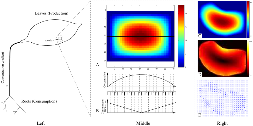
Figure 1: Hormone concentration inside an areole. (left) A rectangular domain (artificial areole) is illustrated with a boundary of c-vascular cells. Assuming c-vascular cells are much more efficient at transporting $s$, the boundary may be taken as a sink and $c$ is governed by Eq. 1. (middle) $c$ at near steady-state, $c_{t}\approx 0$. Also shown are the values of $c$ and $\Delta c$ along a path (in black) across the areole. Notice how the concentration peaks at cells furthest from the veins, while $\Delta c$ peaks near the vein. (right) (C) Concentration, (D) magnitude of gradient, (E) gradient vector field. Observe how the gradient vectors point toward largest concentration increase.

2.3 Analysis of the Poisson Model

2.3.1 Definitions and Background: Geometry

A collection of ground cells surrounded by c-vascular cells is called an areole. Our technical result will assume that an areole is a discretization of a continuous portion of $\mathbb{R}^{2}$ which we call a shape.

Definition 2.

A shape is any subset $\Omega\in\mathbb{R}^{2}$ which is the closure of a bounded open set and has a boundary $\partial\Omega$ consisting of finitely many smooth curves.

A point $Q\in\partial\Omega$ is concave if for any line $\ell$ locally tangent to $Q$ there is an open ball $B_{\varepsilon}(Q)$ such that $B_{\varepsilon}(Q)\cap\ell\cap(\Omega-\partial\Omega)=B_{\varepsilon}(Q)\cap\ell-\left\{{Q}\right\}$ (i.e. the line segment is inside $\Omega$). If $B_{\varepsilon}(Q)\cap\ell\cap\Omega\subset\partial\Omega$, then $Q$ is a convex point. The boundary has concave (convex) curvature at concave (convex) points.

Definition 3.

Let $\Omega$ be a shape and $P\in\mathbb{R}^{2}$. The Euclidean distance function on $\Omega$, denoted $\mathcal{E}_{\Omega}$, is

$$\mathcal{E}_{\Omega}(P)=\inf_{Q\in\partial\Omega}\left\|{P-Q}\right\|_{2}$$

The boundary support of $P$, denoted $\mathrm{bsupp}({P};{\partial\Omega})$, is

$$\mathrm{bsupp}({P};{\partial\Omega})=\left\{{Q\in\partial\Omega:~{}\left\|{P-Q}\right\|=\mathcal{E}_{\Omega}(P)}\right\}.$$

The medial axis of $\Omega$, denoted $\mathbf{MA}(\Omega)$, is the set of points $P$ which have two or more closest points on the boundary, i.e.

$$\mathbf{MA}(\Omega)=\left\{{P\in\Omega:\left|{\mathrm{bsupp}({P};{\partial\Omega})}\right|\geq 2}\right\}.$$

where $\left|{\mathrm{bsupp}({P};{\partial\Omega})}\right|$ denotes the cardinality of the set. Note that $\mathbf{MA}(\Omega)$ does not have to be restricted to the shape $\Omega$ and is well-defined on all of $\mathbb{R}^{2}$. Hence, there is an interior medial axis and an exterior one. Here, we will only be concerned with the interior one.

Theorem 4.

Let $\Omega$ be a shape and $P\in\Omega$. Suppose $\left|{\mathrm{bsupp}({P};{\partial\Omega})}\right|=1$ and pick the unique $Q\in\mathrm{bsupp}({P};{\partial\Omega})$. Then,

1. $P\not\in\partial\Omega$ implies

   $$\nabla\mathcal{E}_{\Omega}(P)=\frac{Q-P}{\left\|{Q-P}\right\|}$$

   where $Q-P$ is the vector from $Q\in\partial\Omega$ to $P$.

2. If $\partial\Omega$ is $C^{k}$ at $Q$, then $\nabla\mathcal{E}_{\Omega}$ is $C^{k}$ at $P$.

Proof.

Part (a) is due to [17, 4.8(3)] and (b) is a consequence of the more general result by [23] (see also [25]). ∎

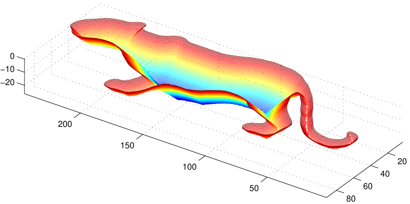
Figure 2: Examples of distance map and medial axis (see [33]). top: negative distance map $-\mathcal{E}_{\Omega}$, center: level sets of $\mathcal{E}_{\Omega}$, bottom: medial axis computed as in [11].

Corollary 5.

$\mathcal{E}_{\Omega}(P)$ is smooth at $P\in\Omega-\mathbf{MA}(\Omega)$.

Proof.

Immediate from Theorem 4(b) and the definition of shape. ∎

Theorem 6.

Let $\Omega$ be a shape. Then

1. $\mathbf{MA}(\Omega)$ has no interior, i.e. it is thin.

2. $\mathbf{MA}(\Omega)$ consists of a finite number of connected piece-wise smooth curves.

3. if $P\in\mathbf{MA}(\Omega)$, $Q\in\mathrm{bsupp}({P};{\partial\Omega})$ and $C$ is the center of curvature for $\partial\Omega$ at $Q$, then $\left\|{P-Q}\right\|\leq\left\|{C-Q}\right\|$ whenever $\left\|{C-P}\right\|\leq\left\|{C-Q}\right\|$.

Proof.

Part (i) is shown in [26] and in [5]; (ii) is treated in detail by [7]. Part (iii) asserts that if a medial axis point is inside the circle of curvature of a point in its boundary support, then it cannot be further than the center of curvature. ∎

Theorem 7.

Let $\Omega$ be a shape. There is a unique $c$ on $\Omega$ such that $c=0$ on $\partial\Omega$ and $\nabla^{2}c=-K/D$.

Proof.

See [8, p. 246] or Theorem 4.3 of [19] for a more general statement and proof. Also see [21]. ∎

Theorem 8 (Divergence).

Let $\partial B_{\varepsilon}(P)$ be a circle or radius $\varepsilon$ centered at $P\in\mathbb{R}^{2}$, $\cal{N}$ the inner normals. Then

$$\nabla^{2}c(P)=\lim_{\varepsilon\to 0}\int_{\partial B_{\varepsilon}(P)}\left<{\nabla c},{N}\right>ds.$$

Proof.

See p. 151 in [40]. ∎

Definition 9.

The $\Theta$-notation for asymptotic behavior of a function is defined as:

$$\Theta(g(n))=\left\{{f(n):\exists c_{1},c_{2},n_{0}~{}\mathrm{positive}~{}s.t.~{}\forall n>n_{0},0\leq c_{1}g(n)\leq f(n)\leq c_{2}f(n)}\right\}.$$

2.3.2 Statement of Result

Result 1 is based on the following theorem.

Theorem 10.

Let $\Omega$ be a shape and $c:\Omega\to\mathbb{R}$ the unique function satisfying $c(x,y)=0$ on $(x,y)\in\partial\Omega$ and

$$\nabla^{2}c=-\frac{K}{D}\quad.$$ (2)

Suppose $P\in\Omega$ is such that $\mathcal{E}_{\Omega}(P)=L=\sup_{\Omega}\mathcal{E}_{\Omega}$ and $Q\in\mathrm{bsupp}({P};{\partial\Omega})$. Suppose the smallest concave curvature radius is $pL$ with $p>0$. Then,

1. $c(Q)\in\Theta(L^{2})$,

2. $\frac{K}{2D}L\leq\left|{\nabla c}\right|\leq\frac{K}{D}L\frac{2p+1}{p}$,

3. $\sup_{\partial\Omega}\left|{\nabla c}\right|>\sup_{\Omega-\partial\Omega}\left|{\nabla c}\right|$

If an areole is regarded as a discretization of a shape $\Omega$, then the discrete approximation behaves as stated in Theorem 10. Observe that $\nabla c$ at $\partial\Omega$ is perpendicular to the boundary because $c=0$ there; hence, $\nabla c(Q)$ points in the direction of $P$ according to Theorem 4.

2.3.3 Organization of the Proof

Parts (a) and (b) of Theorem 10 follow from Lemma 20. The idea of the proof is to find appropriate bounding functions, one from below $v$ and another $u$ from above, that sandwich the unique solution $c$ and that take the same values at the boundary. Thus, $v\leq c\leq u$ everywhere and $\left|{\nabla v}\right|\leq\left|{\nabla c}\right|\leq\left|{\nabla u}\right|$ on points where $v=c=u$, i.e. the boundary. Since the value of $c$ must be the same at the boundary, its gradient there must be perpendicular to the boundary which gives the direction as claimed in Result 1(b). Lemma 14 and Lemma 18 give the lower bound and upper bound constructions and Lemma 20 collects them.

Part (c) of Theorem 10 is necessary to show that the c-vascular strand creation process is well defined. Result 1(c) is the non-technical version of this claim which is stated more precisely in Lemma 21. The proof is based on the idea that the boundary may be seen as evolving by considering level sets of $c$, i.e. points $\gamma_{c_{0}}$ where $c(x,y)=c_{0}$. The gradient must be perpendicular to this level set and the solution of Eq. 2 inside it follows the same constraints as the shapes on which the problem is defined. We may move the level set curve $\gamma_{c_{0}}$ so that the point on $\gamma_{c_{0}}$ which is on the gradient curve initiated at the point $Q$ of maximal gradient on $\gamma_{0}$ touches $Q$ for small enough $c_{0}$. Knowing that the solution on the smaller shape must be strictly smaller than on the original shape shows that the maximum gradient magnitude must be strictly decreasing as the curve evolves. This is true for all curves, including the evolved ones (i.e. $\gamma_{c_{1}}$ for $c_{1}>c_{0}$), so the gradient in the interior of the shape must be lower than the maximum on the boundary.

2.3.4 The Proof

We begin with Lemma 11 which will be used (indirectly) in most of the proofs that follow. It states that a discretization of the dynamic process will always move the concentration values in the same direction (up or down) if this direction is locally the same for all discrete points. This fact will be used to prove the next result, Lemma 12, which states that the equilibrium solution over a shape completely contained in another shape will be bounded above by the solution over the larger shape. This holds even if the initializing function is not smooth.

Lemma 11.

Let $c_{t}=D\nabla^{2}c+K$ be approximated on a square lattice by $p_{i}$ and its four neighbors $n_{j}$ by $\tilde{c}_{t}=\frac{D}{h^{2}}\left({\sum_{j}c(n_{j})-4c(p_{i})}\right)+K$ where $h$ is the lattice spacing. Suppose that $\tilde{c}_{t}\leq(\geq)0$ everywhere on the domain of definition at time $t_{0}$. Then

1. $c+\tau\tilde{c}_{t}$ will also satisfy the inequality if $0<\tau\leq\frac{h^{2}}{4D}$; and

2. the discrete dynamics with such $\tau$ make $c$ decrease (increase) monotonically everywhere.

Proof.

Part b) follows directly from a). Let $\alpha=D/h^{2}$ and $\Lambda_{p}=\sum_{j=1,4}c(n_{j})-4c(p)$, so $\tilde{c}_{t}(t_{0},p)=\alpha\Lambda_{p}+K$. After the time step $\tau$ the approximation to $c_{t}$ becomes:

$$\begin{array}[]{rcl}\tilde{c}_{t}(t_{0}+\tau)&=&D\nabla^{2}(c+\tau\tilde{c}_{t}(t_{0}))+K\vspace{1ex}\\ &=&\displaystyle\alpha\left({\sum_{j}\left({c(n_{j})+\tau\tilde{c}_{t}(t_{0},n_{j})}\right)-4\left({c(p_{i})+\tau\tilde{c}_{t}(t_{0},p_{i})}\right)}\right)+K\vspace{1ex}\\ &=&\displaystyle\alpha\left({\Lambda_{p_{i}}+\tau\left({\sum_{j=1}^{4}\tilde{c}_{t}(t_{0},n_{j})-4\tilde{c}_{t}(t_{0},p_{i})}\right)}\right)+K\vspace{1ex}\\ &=&\displaystyle\alpha\left({\Lambda_{p_{i}}+\tau\left({\sum_{j=1}^{4}(\alpha\Lambda_{n_{j}}+K)-4(\alpha\Lambda_{p_{i}}+K)}\right)}\right)+K\vspace{1ex}\\ &=&\displaystyle\alpha\left({\Lambda_{p_{i}}+\tau\alpha\left({\sum_{j=1}^{4}\Lambda_{n_{j}}-4\Lambda_{p_{i}}}\right)}\right)+K\vspace{1ex}\\ &=&\displaystyle\alpha\Lambda_{p_{i}}(1-4\tau\alpha)+\alpha\tau\alpha\sum_{j=1}^{4}\Lambda_{n_{j}}+K\vspace{1ex}\\ \end{array}$$

Now, all of the $\alpha\Lambda_{n_{j}}+K\leq 0$ and $\alpha\Lambda_{p_{i}}+K\leq 0$ by assumption. Also, $0<4\tau\alpha\leq 1$. So choosing the largest $\Lambda_{n_{j}}$ and replacing for the other three bounds the value above (since $\Lambda_{n_{j}}<0$), shows that $\tau$ is used in a linear interpolation between two non-positive numbers. This finishes the claim. ∎

Lemma 12.

Let $u_{t}=D\nabla^{2}u+K=0$ over $\Omega$ with $u=0$ on $\partial\Omega$. If $\Omega^{\prime}\subset\Omega$ and $D\nabla^{2}c+K=0$ on $\Omega^{\prime}$ with $c=0$ on $\partial\Omega^{\prime}$ then $c\leq u$ on $\Omega^{\prime}$. If $\Omega\not\subset\Omega^{\prime}$, then $c<u$ everywhere on $\Omega^{\prime}-\partial\Omega^{\prime}$.

Proof.

If $u=0$ over $\Omega$, then $u_{t}=K>0$ and, by Lemma 11b, $u>0$ in the interior $\Omega-\partial\Omega$ after any non-zero time step. Thus, at equilibrium, $u$ will satisfy the dynamics everywhere on $\Omega^{\prime}$ except possibly on $\partial\Omega^{\prime}$ where it may need to be lower because it the boundary conditions. If a boundary point is lowered in the discretization of the problem, any neighbor will see its $\nabla^{2}u$ decrease and strictly decrease if the neighbor is not moved. This holds at any time step and will affect all points after sufficiently long time because they are all connected. If $\Omega\not\subset\Omega^{\prime}$, then $u$ is not a solution ($u>0$ somewhere on $\partial\Omega^{\prime}$) and the dynamics on $\Omega^{\prime}$ will strictly monotonically lower it everywhere. ∎

Now we show what the solution looks like in one dimension, Lemma 13, and then we turn to two special shapes: the circle (Lemma 14) and the open doughnut (Lemma 15). These shapes will be instrumental in providing the lower and upper bounds needed later on.

Lemma 13.

Suppose the domain is the segment $[0,L]$, ${c_{1D}}(0)=0$ and ${c_{1D}}^{\prime}(L)=0$. Then the solution to Eq. 2 is

$${c_{1D}}(r)=\frac{K}{D}\left({-\frac{r^{2}}{2}+rL}\right)$$

Proof.

By inspection since the solution is unique: $\partial^{2}/(\partial r)^{2}[{c_{1D}}(r)]=-K/D$. ∎

Lemma 14 (Disc).

Let the shape be a circle of radius $L$ centered at the origin. Suppose $c(x,y)=0$ on the boundary where $x^{2}+y^{2}=L^{2}$. Then the solution to Eq. 2 is

$$c(x,y)=\frac{1}{2}{c_{1D}}\left({L-\sqrt{x^{2}+y^{2}}}\right)$$

and

$$\left|{\nabla c(x,y)}\right|=-\frac{1}{2}\frac{K}{D}\sqrt{x^{2}+y^{2}}$$

Proof.

By inspection since the solution is unique. We see that $c_{xx}=c_{yy}=-\frac{1}{2}K/D$, so Eq. 2 is satisfied. ∎

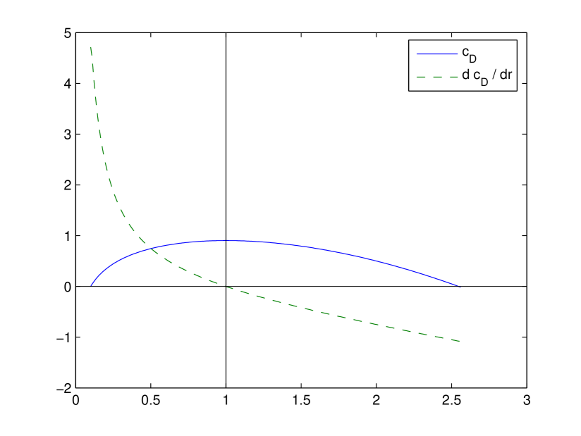
Figure 3: A plot of $c_{D}(r;0.1,0.9)$ and $\frac{dc_{D}}{dr}$. Notice that $c_{D}$ is increasing from $l$ to $l+L$.

Lemma 15 (Open Doughnut).

Let $0\leq l<l+L$ be the radii of two circles centered at the origin. Suppose $c(x,y)=0$ on the boundary $x^{2}+y^{2}=l^{2}$ and $\nabla c(x,y)=0$ for $x^{2}+y^{2}=(l+L)^{2}$. Then the solution to Eq. 2 is

$$c(x,y)=c_{D}\left({\sqrt{x^{2}+y^{2}}}\right)$$

where

$$c_{D}(r)=c_{D}(r;l,L)=\frac{K}{D}\left({\frac{1}{4}\left({l^{2}-r^{2}}\right)+\frac{1}{2}{\ln\left({\frac{r}{l}}\right)}(l+L)^{2}}\right)$$ (3)

Further, $c(x,y)\geq 0$ for $l^{2}\leq x^{2}+y^{2}\leq(l+L)^{2}$.

Proof.

By inspection since the solution is unique. Since $c=0$ at the inner boundary and $\nabla c$ points radially toward the outer boundary, the values of $c$ are increasing radially in $l^{2}\leq x^{2}+y^{2}\leq(l+L)^{2}$. ∎

The next two results (Lemma 16 and Lemma 17) are technical assertions used in the proof of the Upper Bound Lemma (Lemma 18). This is the last result needed to prove Lemma 20 and, therefore, parts (a) and (b) of Theorem 10.

Lemma 16.

Let $\Omega$ be a shape $P\in\Omega$, and $Q\in\mathrm{bsupp}({P};{\partial\Omega})$. Let $\Sigma$ be the circle of curvature of $\Omega$ at $Q$. Then $\mathcal{E}_{\Omega}(P^{\prime})=\mathcal{E}_{\Sigma}(P^{\prime})+O(\varepsilon^{3})$ for $\left\|{P-P^{\prime}}\right\|=\varepsilon$, and over a circular region $R$ of radius $\varepsilon$ centered at $P$

$$\lim_{\varepsilon\to 0}\frac{1}{\pi\varepsilon^{2}}\int_{\partial R}\left<{\frac{\partial}{\partial r}c_{D}(\mathcal{E}_{\Omega})\nabla\mathcal{E}_{\Omega}},{\mathcal{N}}\right>ds=\lim_{\varepsilon\to 0}\frac{1}{\pi\varepsilon^{2}}\int_{\partial R}\left<{\frac{\partial}{\partial r}c_{D}(\mathcal{E}_{\Sigma})\nabla\mathcal{E}_{\Sigma}},{\mathcal{N}}\right>ds$$

Proof.

Write the second order approximation $\mathcal{E}_{\Omega}=\mathcal{E}_{\Sigma}+O(\varepsilon^{3})$ and $\nabla\mathcal{E}_{\Omega}=\nabla\mathcal{E}_{\Sigma}+O(\varepsilon^{2})$. In a circular neighborhood $R$, the limit becomes:

$$\lim_{\varepsilon\to 0}\frac{1}{\pi\varepsilon^{2}}\int_{0}^{2\pi\varepsilon}\left<{\frac{\partial}{\partial r}c_{D}(\mathcal{E}_{\Omega})\nabla\mathcal{E}_{\Omega}},{\mathcal{N}}\right>ds=\lim_{\varepsilon\to 0}\int_{0}^{2\pi}\frac{1}{\pi\varepsilon}\left<{\frac{\partial}{\partial r}c_{D}(\mathcal{E}_{\Omega})\nabla\mathcal{E}_{\Omega}},{\mathcal{N}}\right>ds$$

Now, $\frac{\partial}{\partial r}c_{D}(\mathcal{E}_{\Sigma}+O(\varepsilon^{3}))=\frac{\partial}{\partial r}c_{D}(\mathcal{E}_{\Sigma})+O(\varepsilon^{3})$ by inspection of $\frac{\partial}{\partial r}c_{D}(r)$, which gives:

$$\begin{array}[]{rcl}\frac{1}{\pi\varepsilon}{\frac{\partial}{\partial r}c_{D}(\mathcal{E}_{\Omega})\nabla\mathcal{E}_{\Omega}}&=&\frac{1}{\pi\varepsilon}{\frac{\partial}{\partial r}c_{D}(\mathcal{E}_{\Sigma}+O(\varepsilon^{3}))\left({\nabla\mathcal{E}_{\Sigma}+O(\varepsilon^{2})}\right)\vspace{1ex}}\\ &=&\frac{1}{\pi\varepsilon}\left({\frac{\partial}{\partial r}c_{D}(\mathcal{E}_{\Sigma})\nabla\mathcal{E}_{\Sigma}+\frac{\partial}{\partial r}c_{D}(\mathcal{E}_{\Sigma})O(\varepsilon^{2})+O(\varepsilon^{3})\nabla\mathcal{E}_{\Sigma}+O(\varepsilon^{5})}\right)\vspace{1ex}\\ &\to&\displaystyle\lim_{\varepsilon\to 0}\frac{1}{\pi\varepsilon}\frac{\partial}{\partial r}c_{D}(\mathcal{E}_{\Sigma})\nabla\mathcal{E}_{\Sigma}\end{array}$$

∎

Lemma 17.

Suppose the shape $\Omega$ is the disc as in Lemma 14 with radius $l+L$ and $c$ is the solution. Then,

$$u(x,y)=c_{D}(l+L-\sqrt{x^{2}+y^{2}})$$

satisfies $\nabla^{2}u<\nabla^{2}c=-K/D$ for all points except the center.

Proof.

Write $f=u-c$ where $c$ is the solution for the disc from Lemma 14. Letting $R(x,y)=\sqrt{x^{2}+y^{2}}$

$$\begin{array}[]{rcl}f(R(x,y))&=&c_{D}(l+L-R)-\frac{1}{2}{c_{1D}}(l+L-R)\vspace{1ex}\\ &=&\frac{K}{D}\left({\frac{l^{2}}{4}+\frac{1}{2}\left({\ln\left({\frac{l+L-R}{l}}\right)(l+L)^{2}-(l+L-R)(l+L)}\right)}\right)\end{array}$$

A direct calculation shows that

$$\nabla^{2}f(x,y)=-\frac{1}{2}\frac{K}{D}\frac{l+L}{\sqrt{x^{2}+y^{2}}}$$

which demonstrates that $f(r)<0$ everywhere and $\lim_{r\to 0}f(r)=-\infty$ in the center of the disc. Therefore, $\nabla^{2}~{}u~{}=~{}\nabla^{2}~{}f~{}+~{}\nabla^{2}c<-K/D$ because $\nabla^{2}c=-K/D$. ∎

Lemma 18 (Upper Bound).

Let the conditions of Theorem 10 hold. Define $u(x,y)=2c_{D}(l+\mathcal{E}_{\Omega}(x,y))$ with $l=pL$. Then $u\geq c$.

Proof.

We shall show that any discretization $\tilde{u}$ with spacing $h<h_{0}$ (for some $h_{0}>0$) of $u$ will satisfy $D\nabla^{2}\tilde{u}+K\leq 0$. Thus, Lemma 11 shows that a dynamical process initialized with $u$ will decrease $u$ everywhere with each time step and, by Theorem 7, it should converge to $c$. Hence, $c\leq u$.

First, we treat non-medial axis points. Let $P=(x,y)\in\Omega$ (not on the medial axis) and $Q\in\partial\Omega$ which is closest to $P$, i.e. $\left\|{P-Q}\right\|=\mathcal{E}(P)$. Suppose $\partial\Omega$ near $Q$ is approximated by the circle of curvature at $Q$. Thus, Lemma 16 applies and, by the Divergence Theorem 8, $\nabla^{2}u(P)$ is the same as if the boundary were a circle at $Q$. Following Theorem 6 MA2, there are three cases: (a) $P$ outside the circle, (b) $P$ inside, and (c) the circle has infinite radius – it is a line segment. Lemma 15 shows that $\nabla^{2}u(P)=-2K/D<-K/D$ which takes care of (a), and (b) is covered by Lemma 17. If the boundary is locally a straight line, then

$$\nabla^{2}u=\frac{\partial^{2}}{\partial r^{2}}2c_{D}(l+r)=-\frac{K}{D}\left({1+(l+L)^{2}/r^{2}}\right)$$ (4)

with $l<r<l+L$ and $r$ is in the direction of the gradient. So, $\nabla^{2}u(P)<-K/D$ for all $P\in\Omega-\mathbf{MA}(\Omega)$.

Now suppose that the of $u$ on $\Omega$ are sampled on a discrete square lattice with spacing $h>0$. There, $\nabla^{2}u(p)$ is approximated by the formula for $\Lambda_{p}$ in the proof of Lemma 11. The error of the approximation is $O(h^{2})$ (see [1]). Thus, from the above, $h$ may be chosen so that $\Lambda^{u}_{P}<-K/D$ for $P\in\Omega$ further than $h$ from $\mathbf{MA}(\Omega)$.

Let $\mathcal{E}_{\Sigma_{P}}$ to be the distance function from the circle of curvature at the boundary point corresponding to $P\not\in\mathbf{MA}(\Omega)$. Hence, if $\left\|{P^{\prime}-P}\right\|=h$, then $\mathcal{E}_{\Sigma_{P}}(P^{\prime})=\mathcal{E}_{\Omega}(P^{\prime})+\varepsilon_{P^{\prime}}$ where $\varepsilon_{P^{\prime}}=O(h^{3})$. Set

$$\varepsilon_{P}=\sup_{\left\|{P^{\prime}-P}\right\|=h}\left|{\varepsilon_{P^{\prime}}}\right|\quad\mathrm{and}\quad\varepsilon=\sup_{P\in\Omega-\mathbf{MA}(\Omega)}\varepsilon_{P^{\prime}}$$

where $0\leq\varepsilon<h$ for small enough $h$. So, choose such an $h$ and define

$$u_{h}(x,y)=2c_{D}(l+\mathcal{E}_{\Omega}(x,y);l,L+2h)$$

and notice that we may refine the grid (i.e. choose $h$ smaller) and the above properties will still hold. Thus, refine $h$ if necessary to make $\Lambda^{u_{h}}_{P}<-K/D$ on shape points further than $h$ from the medial axis. Refine it further to $\Lambda^{u_{h}}_{P}<-K/D$ on an open doughnut with $l$ inner radius and $L+2h$ outer radius. Make sure that $h$ is small enough so that $c_{D}(r+h)-2c_{D}(r)+c_{D}(r-h)<-K/D$ (this is needed in the tangent line construction below), which is possible because of Eq. 4.

Now we show that this also makes $\Lambda^{u_{h}}_{P}<-K/D$ for points on the medial axis and those closer than $h$ from it. Pick such a $P$ and let consider $Q\in\mathrm{bsupp}({P};{\partial\Omega})$. If $Q$ is concave, then approximate the boundary by its circle of curvature and look at $u_{h}^{\Sigma}=2c_{D}(l+\mathcal{E}_{\Sigma}(x,y);l,L+2h)$ . A neighbor $N$ of $P$ used in $\Lambda^{u_{h}}_{P}$ satisfies $\mathcal{E}_{\Sigma}(N)\geq\mathcal{E}_{\Omega}(N)$ (because $Q$ is concave and the difference is no more than $\varepsilon$. Hence, $u_{h}^{\Sigma}(N)\geq u_{h}(N)$ since $c_{D}$ is increasing until $l+L+2h$. Further, $\mathcal{E}_{\Sigma}(P)=\mathcal{E}_{\Omega}(P)$ because the circle of curvature touches $\partial\Omega$ at $Q$. Hence, $\Lambda^{u_{h}}_{P}<\Lambda^{u^{\Sigma}_{h}}_{P}<-K/D$ because $P$ is not a medial axis point for $\Sigma$.

If, on the other hand, there is a concave $Q\in\mathrm{bsupp}({P};{\partial\Omega})$, then instead of the circle of curvature we may take the tangent line $\ell_{P}$ at $Q$ define $\mathcal{E}_{\ell_{P}}$ exactly similarly to $\mathcal{E}_{\Sigma_{P}}$ above. Refine $h$ so that any point $P^{\prime}$ for which $\left\|{P-P^{\prime}}\right\|=h$ is closest to a point $Q^{\prime}\in\ell_{P}$ that lies outside the $\Omega$ or on $\partial\Omega$.. Thus, as before, $\mathcal{E}_{\ell_{P}}(N)\geq\mathcal{E}_{\Omega}(N)$ for any $N$ near $P$, i.e. $\left\|{N-P}\right\|=h$. Therefore, $\Lambda^{u_{h}}_{P}<\Lambda^{u^{\Sigma}_{h}}_{P}<-K/D$.

Finally, Lemma 12 shows that $u_{h}>c$ from which we conclude that $u\geq c$ since $\lim_{h\to 0}u_{h}\to u$. ∎

Remark 19.

The function $u(x,y)$ need not be smooth on $\Omega$. In fact, it will fail to have fist derivatives on the medial axis of most shapes.

Lemma 20.

Let the conditions of Theorem 10 hold. Then $c=\Theta(L^{2})$. Further, if $P$ is the center of the largest inscribed circle and $Q$ a point on the boundary of the shape and the circle, then $\nabla c(Q)$ points toward $P$ and

$$\frac{K}{2D}L\leq\left|{\nabla c}\right|\leq\frac{K}{D}L\frac{2p+1}{p}.$$

Proof.

The Disc Lemma 14 gives the lower bound function and the Upper Bound Lemma 18 the rest. The gradient points in the direction of the normal to the boundary because $c=0$ on $\partial\Omega$. The magnitude follows from a simple calculation of $\partial/\partial r[c_{D}(r)]$ at $r=pL$ (see the Open Doughnut Lemma for the definition of $c_{D}(r)$). ∎

Finally, the following result completes the proof of Theorem 10.

Lemma 21 (Decreasing Gradient).

Let $c$ satisfy the Poisson equation (Eq. 2) on $\Omega$ and $c=0$ on $\partial\Omega$. Then

$$M=\sup_{\Omega}\left|{\nabla c}\right|=\sup_{\partial\Omega}\left|{\nabla c}\right|$$

and

$$\left|{\nabla c(x,y)}\right|<M,\quad(x,y)\in\Omega-\partial\Omega~{}.$$

Proof.

Let $\gamma_{c_{0}}=\left\{{(x,y)\in\Omega:c(x,y)=c_{0}}\right\}$. A number $0<c_{0}<\sup_{\Omega}c$ must exist since $c>0$ on $\Omega-\partial\Omega$ by Lemma 11b. Let the shape $\Omega^{\prime}$ be defined by $(x,y)\in\Omega$ such that $c(x,y)\geq c_{0}$. Hence, $\Omega^{\prime}\subset\Omega$ and $\Omega\not\subset\Omega^{\prime}$. The boundary $\partial\Omega^{\prime}=\gamma_{c_{0}}$ is regular, so there is a unique $v$ satisfying Eq. 2 on $\Omega^{\prime}$ with $v=0$ on $\partial\Omega^{\prime}$. Thus, $v=c-c_{0}$ and $\nabla v=\nabla c$ on $\Omega^{\prime}$.

Thus, $\gamma_{0}=\partial\Omega$ and $\gamma_{c_{0}}$ is connected for small enough $c_{0}$ (because $\Omega$ is the closure of an open set). Further, if $c_{0}<\varepsilon_{0}$ for some $\varepsilon_{0}>0$, then $\gamma_{c_{0}}$ is a smooth curve because $\nabla_{\gamma_{c_{0}}}c=0$ on $\gamma_{c_{0}}$, $c$ is at least twice differentiable, and $\nabla c\neq 0$ when taken over $\Omega$ on points of $\gamma_{0}$. In fact, $\nabla c$ is perpendicular to the curve $\gamma_{0}=\partial\Omega$. Let $Q\in\gamma_{0}$ be such that $\nabla c(Q)=\sup_{\partial\Omega}\left|{\nabla c}\right|$. Let $\beta$ be the integral curve segment starting at $\beta(0)=Q$ with tangents in the direction of $\nabla c$ and such that $\beta(1)\in\gamma_{c_{0}}$. Since $\nabla c$ is perpendicular to $\gamma_{0}$, $\beta(1)$ will be the closest point to $\gamma_{0}$ from $\gamma_{c_{0}}$ for small enough $c_{0}$. Thus, $\gamma_{c_{0}}$ may be translated so that $\beta(1)$ touches $Q$ ensuring that $\gamma_{c_{0}}$ is completely contained in $\Omega$; denote this translated curve by $\gamma_{c_{0}}^{\prime}$.

The solution $v^{\prime}$ to Eq. 2 on $\gamma_{c_{0}}^{\prime}$ and its interior must be the translated $v$. By Lemma 12 $v^{\prime}<c$ everywhere except on $\gamma_{0}\cap\gamma_{c_{0}}^{\prime}$ (e.g. at $Q$) where $v^{\prime}=c$. Hence, $\left|{\nabla v^{\prime}(Q)}\right|<\left|{\nabla u(Q)}\right|$. Therefore, $\left|{\nabla u(Q)}\right|$ is strictly decreasing in the direction of $\nabla u(Q)$.

(a)	(b)	(c)

Figure 4: Level sets of $c$. (a,b) Rectangular shape. (c) Areole from [31].

∎

3 Proportional Destruction Hypothesis: Helmholtz Model

3.1 Background

In [15] we noted that new veins may emerge simultaneously in areoles of drastically different sizes. We argued that the most parsimonious explanation of this phenomenon is that auxin is produced at a rate that is constant for each cell, regardless of that cell’s size. But we did not develop the question of auxin destruction beyond assuming that veins drain the hormone in such a way that it is effectively depleted from the areole. A more natural assumption emerges from considering recent molecular work.

Auxin is involved in a variety of processes that take place in plant cells at all times, so a portion of the free IAA is constantly being depleted. For example, it has recently been shown [22, 10] that the early response genes are activated by auxin through an increased degradation of promoter inhibitors. Thus, auxin binds to a TIR1 protein which is instrumental in tagging inhibitor proteins (Aux/IAA) for degradation: the larger the concentration of auxin, the more effective the degradation. In addition, the hormone “is readily conjugated to a wide variety of larger molecules, rendering it inactive. Indeed, the majority of IAA in the plant is in the form of inactive conjugates. Auxin conjugation and catabolism can therefore decrease active auxin levels.” [35, p. 853]. For these reasons, we propose the Proportional Destruction Hypothesis:

Hypothesis 2 (Proportional Destruction).

Free auxin levels are constantly being depleted at a rate proportional to the available hormone levels.

The constant of proportionality will be denoted by $\alpha$ and referred to as the destruction constant.

3.2 Helmholtz Model Definition

Helmholtz Model Definitions Ground Cell: Diffusion coefficient $D_{g}$; production $\rho=K/S$. C-Vascular Cell: At least one interface has diff. coef. $D_{v}>D_{g}$; production $\rho=K/S$. Cell Functions (Program) CF1: Produce substance $s$ at constant rate $K$ and destroy it at a rate $\alpha c$. CF2: Measure $c$ and $\Delta c$ through interfaces. CF3: Diffuse $s$ through interfaces. CF4: When $\Delta c>\tau$ through interface $I$, change its diffusion coefficient to $D_{v}$.

Table 2: Helmholtz model. Terms definitions: $K$ is the per-cell substance production rate (mass/time); $S$ is the size of the cell (volume); $\rho$ is the per-volume production rate; $D_{x}$ are diffusion coefficients related to the permeability of cell interfaces; $c$ is the concentration of the substance inside the cell, $\alpha$ is the destruction constant, and $\Delta c(I)$ is the difference of concentration through the interface $I$; $\tau$ is a threshold.

The Proportional Destruction Hypothesis leads to the updated formulation of our model shown in Table 2. We shall assume that the only mode of auxin transport is diffusion according to Fick’s Law. Our constant production of $K$ (kg$\cdot$s^-1) is replaced by a speed of increase in concentration equal to $K/S(i)$ where $S(i)$ is the size of cell $i$. The proportional destruction of auxin implies a decrease in concentration given by $-\alpha m(i)/S(i)=-\alpha c(i)$ with $c(i)$ denoting concentration. Therefore, the manner in which the auxin concentration changes with time within each cell can be written as:

$$\frac{\partial c}{\partial t}=D\nabla^{2}c+\frac{K}{S}-\alpha c~{}.$$ (5)

The equilibrium of this dynamical system, when $c_{t}=0$, is therefore described by an inhomogeneous Helmholtz equation, which is why we refer to this formulation as the Helmholtz Model.

3.3 Analysis of the Helmholtz Model

It turns out that this relatively small modification to the Poisson model greatly improves the model’s descriptive power. We now establish the mathematical results that make this claim concrete before we turn to the discussion of biological experiments in the next section. We demonstrate that the same type of distance information is captured by the Helmholtz model in Proposition 22 and Proposition 24, but that it can be obtained in more than one fashion if the destruction constant is small. If this constant is large, we show that a different kind of distance becomes available to the discrete system – one given by the logarithm of concentration.

Proposition 22.

Consider the dynamical system

$$\frac{\partial{c}}{\partial{t}}=D\nabla^{2}c+\rho_{\Omega}-\alpha c.$$ (6)

Suppose that it acts over a domain $\Omega$ which a shape as in Theorem 10 and on which we impose a zero-flux boundary condition (Neumann). Let $\rho_{\Omega}:\Omega\to\mathbb{R}$. Then the following holds.

1. If $\alpha>0$, then $\lim_{t\to\infty}c=c_{\alpha}$ for a unique steady-state $c_{\alpha}$.

2. Let $\alpha=0$ and $R=\int\rho_{\Omega}\mathrm{d}{\Omega}/\int\mathrm{d}{\Omega}$ be the average production. Then $\lim_{t\to\infty}c_{t}=R$ and $c$ converges to $c_{\alpha}+\mathrm{cst.}$ whenever $R=0$. Further, $\nabla c_{\alpha}$ is unique even when $R\neq 0$.

3. If $A,B\in\mathbb{R}$, then the transformation $\rho_{\Omega}\mapsto A\rho_{\Omega}+\alpha B$ induces a unique transformation of the steady state $c_{\alpha}\mapsto Ac_{\alpha}+B$ and vice versa. It follows that the gradient of $c_{\alpha}$ is only affected if $A\neq 1$: $\nabla c_{\alpha}\mapsto A\nabla c_{\alpha}$.

Remark 23.

In part (c), if the destruction term is not linear, e.g. $\alpha c+\beta c^{2}$, then the gradient might be affected by $B$ as well.

Proof.

Parts (a) and (b). To show existence we prove that the dynamical system achieves $c_{t}=0$. Consider the dynamical system $c_{tt}=D\nabla^{2}c_{t}-\alpha c_{t}$. The boundary conditions are inherited: since no flux goes through the boundary, there must be no change of concentration in time, i.e. $\nabla c_{t}\cdot\mathbf{n}=0$ on $\partial\Omega$. The unique solution of this system is $c_{t}=0$.

To prove uniqueness, suppose $u_{1}$ and $u_{2}$ both satisfy the equation given the boundary conditions and $c_{t}=0$. Thus

$$D\nabla^{2}u_{1}+\rho_{\Omega}-\alpha u_{1}=D\nabla^{2}u_{2}+\rho_{\Omega}-\alpha u_{2}$$

which gives rise to $D\nabla^{2}v-\alpha v=0$ where $v=u_{1}-u_{2}$ and $\nabla v\cdot\mathbf{n}=0$ where $\mathbf{n}$ is the normal to the boundary. Since $v$ is elliptic and $\alpha>0$, $v$ vanishes everywhere and uniqueness follows (see [8, p. 329 and 321]). The same reference shows that if $\alpha=0$, then this uniqueness is up to an additive constant $u=u_{1}+\mathrm{cst}$; that is, only $\nabla u$ is unique.

Now to show the convergence in (b) whenever $R=0$, note that $c_{tt}=D\nabla^{2}c_{t}$ assuming $\alpha=0$. This has a steady-state s.t. $c_{t}=\mathrm{cst.}$ everywhere. Also, $\int c_{t}=\int\rho_{\Omega}\mathrm{d}{\Omega}$ which shows that $c_{t}=R$.

Part (c). Let $c_{\alpha}$ satisfy Eq. 6 for $c_{t}=0$ and a production function $\rho^{(\alpha)}_{\Omega}$. Then, $D\nabla^{2}c_{\alpha}-\alpha c_{\alpha}=-\rho^{(\alpha)}_{\Omega}$. Suppose $c=Ac_{\alpha}+B$ satisfies the equation for some $\rho_{\Omega}$. Since this $c$ is unique, the following verification proves the claim.

$$\begin{array}[]{cl}&D\nabla^{2}c-\alpha c=-\rho_{\Omega}\\ \therefore&D\nabla^{2}(Ac_{\alpha}+B)-\alpha(Ac_{\alpha}+B)=-\rho_{\Omega}\\ \therefore&AD\nabla^{2}c_{\alpha}-A\alpha c_{\alpha}-\alpha B=-\rho_{\Omega}\\ \therefore&A(D\nabla^{2}c_{\alpha}-\alpha c_{\alpha})=-\rho_{\Omega}+\alpha B\\ \therefore&A(-\rho^{(\alpha)}_{\Omega})=-\rho_{\Omega}+\alpha B\\ \therefore&\rho_{\Omega}=A(\rho^{(\alpha)}_{\Omega})+\alpha B\end{array}$$

The other direction is derived similarly and the result follows. ∎

We can relate the steady-state solution of Eq. 6 with small $\alpha$ to the steady-state solution of the dynamical system in the previous section. In fact, we now show that there are conditions under which the two systems are similar even though the boundary conditions are different. The key difference is that before we assumed a constant value for $c$ at the boundary whereas now we only assume no flow through the boundary. Fig. 5 illustrates the correspondence in 1-D, and the following proposition makes the claim in 2-D precise.

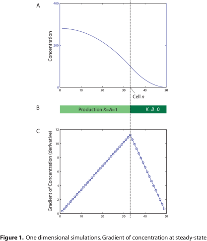
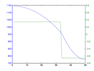
(a)	(b)

Figure 5: Illustration of the steady-state in a 1-D system with two domains of production values and small $\alpha$. (a) Uniform diffusion coefficients. (b) Smaller diffusion coefficients on the left. top: Concentration at equilibrium (blue curve) and production curve (green curve) on y-axis against cell position on x-axis. bottom: Gradient of concentration (or difference in concentration $\Delta c$). Notice that $\Delta c$ attains a maximum where the production (equivalently, cell size) changes abruptly. Observe also that the location of this maximum has similar properties to the location of a sink in 1-D: e.g., the portion in (a) where $K=A=1$ has a parabolic concentration profile with a maximum where the $\Delta c$ is lowest and a minimum where the $\Delta c$ is largest.

Proposition 24.

Let $\Omega$ be a shape with two components $\Omega=\Omega_{0}\cup\Omega_{1}$ such that $\Omega_{0}\cap\Omega_{1}=\partial\Omega_{0}$. Let $D_{0}$ and $D_{1}$ be the diffusion coefficients inside $\Omega_{0}$ and $\Omega_{1}$ respectively. If $\int_{\Omega_{0}}\rho_{\Omega}\mathrm{d}{v}+\int_{\Omega_{1}}\rho_{\Omega}\mathrm{d}{v}=0$ and $\rho_{\Omega}(\Omega_{0})=K\int_{\Omega_{0}}\mathrm{d}{v}>0$, then

$$\lim_{{D_{0}}/{D_{1}}\to 0}c_{\alpha}=c_{K}$$

where $c_{K}$ satisfies Theorem 10 for the shape $\Omega_{0}$ by setting $c_{K}(\partial\Omega_{0})=0$.

Proof.

The convergence of the system derives from Proposition 22(b). As $D_{0}/D_{1}\to 0$ the relative speed of diffusion in $\Omega_{1}$ increases to infinity. Thus, the concentration over $\Omega_{1}$ will tend to a constant and, consequently, so will $c(\partial\Omega_{0})=c(\Omega_{0}\cap\Omega_{1})$. The conditions of Theorem 10 are therefore satisfied and the claim follows. ∎

Note, however, that the destruction constant must be sufficiently small in order to obtain a good correspondence. But the value of $\alpha$ has a more important role. A strictly positive $\alpha$ implies that there is a maximal distance beyond which information cannot travel. Assuming that measurements that cells can perform have a limited precision, our next result shows that the contribution of cell A to the concentration at cell B will be negligible whenever A is sufficiently far from B. The larger the value of $\alpha$, the shorter this distance needs to be.

Theorem 25.

Consider the dynamical system in Eq. 6 and assume the conditions on the domain as in Proposition 22. Let $G(r;\sigma)=\exp(-r^{2}/(2\sigma^{2}))$ and consider the Gaussian convolution kernel $G_{1}=(\sigma^{3}/{2\pi})G(\sqrt{x^{2}+y^{2}};\sigma)$, $\sigma=1/\alpha$. Then

$$\lim_{\alpha\to\infty}(G_{1}\star\rho_{\Omega})=c_{\alpha}$$

where $\star$ denotes convolution and $c_{\alpha}$ is as in Proposition 22.

Proof.

By inspection, $c^{*}=G_{1}\star\rho_{\Omega}$ satisfies Eq. 6 as $\alpha\to\infty$.

Suppose that we have a convolution kernel $G_{2}$ for which $\sigma$ is a function of $\alpha$ and such that $\int_{\Omega}\alpha G_{2}=1$ and $\sigma(\alpha)\to 0$ as $\alpha\to\infty$. Therefore, $G_{2}\star\rho_{\Omega}\to S$ so $S-\alpha(G_{2}\star S)\to 0$. We now show that $G_{1}$ has this property, and that $\nabla^{2}(G_{2}\star S)\to 0$ which shows that

$$\lim_{\alpha\to\infty}D\nabla^{2}c^{*}+\rho_{\Omega}-\alpha c^{*}=0$$

and proves the claim.

The extrema of $G_{xx}=\partial G^{2}/\partial x^{2}$ are at $r=\sqrt{x^{2}+y^{2}}=0,-\sigma\sqrt{3},\sigma\sqrt{3}$. The values are $G_{xx}(0)=-1/\sigma^{2}G(0)=-1/\sigma^{2}$, and $G_{xx}(\sigma\sqrt{3})=2/\sigma^{2}\exp(-3/2)$. Hence, choosing $G_{1}=\sigma^{3}/\sqrt{2\pi}G$ implies that $\sup\left|{\partial G_{1}^{2}/\partial x^{2}}\right|=O(\sigma)$ and that $\int_{\Omega}G_{1}=O(\sigma)$ (because $\int_{\mathbb{R}^{2}}G(\sqrt{x^{2}+y^{2}};\sigma)=1/(\sigma^{2}{2\pi}$). Thus, setting $\alpha=1/\sigma$, we have that $\nabla^{2}(G_{1}\star\rho_{\Omega})=\sigma\to 0$ and that $\int\alpha G_{1}=1$. The claim now follows. ∎

Corollary 26.

Suppose a shape $\Omega$ has two components $\Omega=\Omega_{0}\cup\Omega_{1}$ such that $\Omega_{0}\cap\Omega_{1}=\partial\Omega_{0}$. If $\rho_{\Omega}(\Omega_{0})=0$ and $\rho_{\Omega}(\Omega_{1})=1$, then

$$\lim_{\alpha\to\infty}\frac{\log c_{\alpha}(Q)-\log c_{\alpha}}{\mathcal{E}_{\Omega_{0}}}=cst.>0$$

where $Q\in\partial\Omega_{0}$ and $\mathcal{E}_{\Omega_{0}}$ is the distance function on $\Omega_{0}$.

3.4 Experimental Support of the Helmholtz Model

The principal biological support of our Poisson model is an indirect one: the model produces patterns that are similar to patterns observed in nature. But it does not, for example, predict the concentrations of auxin in any measurable fashion. By contrast, our Helmholtz model does make such predictions and some experimental data is available. Ljung et al. [24, p. 466 and Fig. 1] “observed an inverse correlation between leaf size and IAA concentration that was independent of growth conditions and developmental stage.” They measured the proportion of hormone mass to total leaf mass $p_{IAA}$ (with units pg$\cdot$mg^-1 ) in leaves of different weight, $W$, and obtained data that can be described well by a function $p_{IAA}=AW^{-x}$ where $A$ is a constant and $x$ ranges between 0.72 and 0.98. This suggests that all cells may be producing auxin at the same constant rate if the hormone is depleted proportionally to its concentration. We reason as follows.

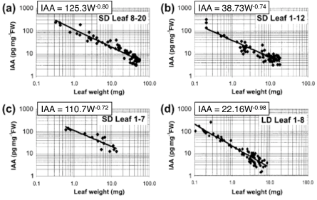
Figure 6: Inverse correlation between leaf size and IAA concentration. After Figure 1 of [24]. SD: short day; LD: long day. Original caption follows. IAA levels in Arabidopsis leaves. The IAA concentration was measured in (a) leaves 8-–20 from six plants grown for six weeks under SD (b) leaves 1–-12 from six plants grown for 4.5 weeks under SD (c) leaves 1–-7 from three plants grown for 3 weeks under SD and (d) leaves 1-–8 from 10 plants grown for 16 days under LD. The data are presented as $\log\log^{-1}$ plots of the IAA concentration in individual leaves versus leaf weight.

Let $m(i)$ denote the mass of auxin in cell $i$ and consider how this quantity changes with time as auxin is produced, destroyed and transported to and from neighboring cells. The production is a constant, $K$, and the destruction, as we argued above, is proportional to the available amounts so this rate of change can be expressed as $m_{t}(i)=K-\alpha m(i)+Transport$. Assuming that the leaf is detached, as it is prior to measurement, the transport term only moves the hormone inside the leaf but does not contribute to either a total increase or a total decrease. Therefore, the rate of change of auxin mass in the whole leaf is $M_{t}=\sum m_{t}(i)=\sum K-\alpha\sum m(i)$. The equilibrium of this system, when $M_{t}=0$, describes well the state of the leaf during measurement because the leaf is small (most leaves are less than 10 mg) and the time needed to perform the manipulations—during which these dynamics apply exactly—is therefore sufficiently long to shift the distribution of the attached leaf to this equilibrium. Consequently, the constant production hypothesis predicts a total auxin mass of around $M_{IAA}=nK/\alpha$ for a leaf with $n$ cells. The quantity reported in the literature, however, is an auxin-to-leaf weight ratio which we calculate to be $p_{IAA}=M_{IAA}/W$. Ljung et al. [24] plot such ratios for four groups of leaves of different sizes against leaf weight. Group members are selected according to the order of leaf emergence (phyllotaxis) and are organized as follows: the first group contains samples from leaf numbers 8–20, the second from leaves 1–12, the third from leaves 1–7, and the fourth from leaves 1–8. Leaves within each of these ranges have a fairly similar final shape and size (Ref. [36]) from which we infer that all leaves in the same group have roughly the same final number of cells. Therefore, since most data points are obtained after cell division has ceased and the cell numbers have stabilized, our analysis suggests that $M_{IAA}$ is roughly the same for all samples in the same group and that only $W$ differs. Theoretically, then, we expect the curves to be described by a function $p_{IAA}=AW^{-x}$ with $A$ a constant and $x=1$ which is in good agreement with the experimentally derived values of $x\approx 0.72,0.74,0.80,0.98$, Fig. 6.

3.5 Further Predictions of the Helmholtz Model

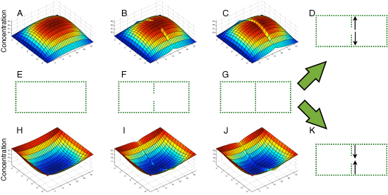
Figure 7: Our schema for the elaboration of new c-vascular strands is unaffected by the relative sizes of boundary cells and interior cells—a consistent difference is enough. However, when all cells perform the functions CF1 and CF3 from Table 2 the equilibrium concentration of $s$ is substantially different for the two types of configuration. (A–C) C-vascular cells are larger than ground cells; (E–G) depiction of c-vascular cells (green squares) as new strands form; (H–J) c-vascular cells smaller than ground cells. (D,K) Arrows show direction of auxin flow. Here $\alpha=0.01$ in all simulations.

3.5.1 Vein Formation

The new (Helmholtz) formulation of the model preserves the distance information available locally to cells under appropriate conditions. Thus, if $\alpha$ is small and there are consistent differences in cell size between ground cells and c-vascular cells, then the distribution of auxin in an areole encodes size information just as it did in the Poisson case (details in Proposition 24). For example, if ground cells are smaller than c-vascular cells (as in Fig. 7A), then the same qualitative distribution of auxin is obtained as in [15]. The program in Table 2 then creates new strands as before. Such relative cell sizes are observed in the early emergence of c-vascular networks (see p. 21 in [28]), but in more mature tissues it is the ground cells that are larger (e.g. the procambium in Fig. 2 of [27] or the mature vein cells compared to others in [30, p. 234] or [29, p. 460]). Our model accommodates this second possibility as well. If boundary cells are smaller than interior cells (as in Fig. 7I), then the hormone distribution will be inverted—higher concentration on the boundary than in the interior—but the differences in concentration between neighboring cells will follow the same qualitative rules as in the first relative size configuration, albeit with an opposite sign (details in Proposition 22). Therefore, the same program can produce new vascular strands and the strands that it produces will be exactly the same in both configurations.

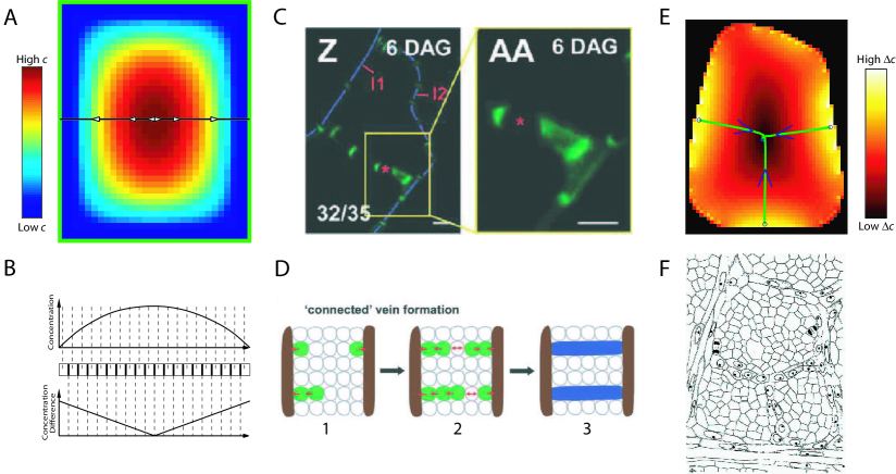
Figure 8: Illustration of the constant production hypothesis and cartoon model for vein formation. (A) Consider a square areole as in Fig. 7A–D in which c-vascular cells are larger than the interior ground cells. Auxin diffuses faster between c-vascular cells than any other type. We show the equilibrium concentration distribution. Note that it is minimal nearest the veins and maximal at the center; i.e., it varies with the distance to the nearest vein. Arrows along a one-dimensional cut (black line through the center) illustrate the flow of auxin along this line from high- to low-concentration pixels. (B) Concentration along the cut in A illustrating maximum at center. Magnitude of gradient (concentration difference between cells) varies “inversely” and peaks at the veins with a value proportional to vein distance to the center. This suggests a schema : differentiate from ground to vascular when gradient magnitude is large (equivalently: when central cells are far from veins). Once a cell begins to differentiate, it clears auxin more efficiently thereby causing adjacent cells to differentiate, until new veins are formed (see D below). (C) PIN1 expression in Arabidopsis. Red star (*) denotes a bipolar cell. (D) Cartoon mechanism of vein formation suggested by Scarpella et al. [32] based on measurements as in C. Note that this realizes precisely the schema in A. (E) Illustration of the veins formed in an areole according to the schema in A and developed in [15]. Note the bipolar flow at single cells predicted by the model and reported in [32]; compare with C. Colors denote magnitude of gradient and arrows show the direction of vascular strand formation, opposite to flow. (F) Cell outlines for the areole modeled in E. Note the large vascular cells. Figure credits: A, B, E from [15]; C, D from Fig. 2 and Fig. 7, resp. of [31]; F from [28].

Fig. 7 shows a simulation of new strands created according to Table 2 in a hypothetical areole for each of the two combinations of relative cell sizes. Notice that the two new c-vascular strands connect in the middle of the areole. They do so by draining $s$ in opposite directions so that the cell where the two strands eventually meet does not have a well defined polarity—it is effectively bipolar. Thus, our model predicts multi-polar cells whenever loops of veins form. Recently at least the bipolar case has been reported for Arabidopsis [32, Fig. 2], Fig. 8 compares our predictions to the empirical observations.

However, our theory explains this phenomenon only under the assumption that vascular cells are larger than ground cells. If these relative sizes are reversed, then we should expect bipolar cells to form but the definition needs to be revised. In effect, the relevant cells would not have carriers facilitating export; instead, neighboring cells from opposite sides of a bipolar cell both exhibit facilitated transport toward the bipolar cell. Our theory predicts that such configurations would arise if new vascular strands are created in more mature organs, extending an existing vein as opposed to existing procambium (e.g. a tertiary vein stemming from a primary may be a good candidate).

3.5.2 Auxin Distribution in Arabidopsis Roots

Roots have a much simpler cell size distribution than leaves, and reliable estimates are easier to obtain. There even exist detailed 3-D models of root tips of Arabidopsis, but we shall only use 2-D slices to test our theory in those organs. This type of data is representative of the full 3-D organ because roots are radially symmetric: rotating the 2-D slice about its long axis yields a good approximation the complete root. Along the same axis, three regions are distinguished: (1) a division zone (DZ) near the tip, (2) an elongation zone immediately adjacent to the DZ, and (3) a maturation or differentiation zone ([29, p. 436], [30]). On average, cells are smallest in the division zone, followed by slightly larger ones in the elongation zone, and then by the largest cells in the maturation zone.

This schematic configuration is depicted in Fig. 9A and forms the setup of the first type of root simulations. Each cell is represented by a rectangular box containing a single dot inside, the unit of auxin production independent of cell size. Note that the hormone distribution obtained predicted in this fashion (Fig. 9B,E) qualitatively agrees with the empirical measurements (Fig. 9C,D) reported by Bhalerao et al. [2]. Their data come from slices of untreated plants and consist of the average concentration of IAA as a function of distance from the root tip. The technique for measuring auxin levels gives good concentration estimates but has poor spatial resolution, so our comparison is restricted to the overall shape of the curve. The use of staining techniques, on the other hand, promises higher resolution but only provides qualitative information. Thus, we suspect that there is a peak of auxin concentration near the root tip, as shown in Fig. 10C, but do not know its height. This observation may be sufficiently explained by the geometry of the organ, as our first schematic simulation suggests, so we turn to a real root specimen to test this claim.

Our next simulation uses a manually traced 2-D slice [6, Fig. 1A] to predict the shape of auxin distribution inside that root. The setup is redrawn in Fig. 10A. Notice that the simulation result (in part B) reproduces that peak. This is a robust feature of the model as the only external cue has been cell size: the diffusion coefficients are all equal, the per-cell auxin production is constant.

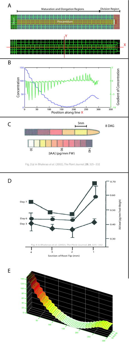
Figure 9: Simulations in a schematic root. (A) Setup inspired by known regions of plant roots [29, p. 434-6]. Cells are rectangular boxes which increase in size from the tip toward the shoot. A single dot inside each cell represents one unit of hormone production; green boundaries (cell interfaces) have the same diffusion coefficients everywhere. (B) Result of simulation. Concentration at steady-state through the horizontal red line in A. (C,D) Measurements of auxin concentration in sampled root tissues (either 5mm or 1mm cylinders) reported by Bhalerao et al. [2, Figs. 2 and 4]. (E) Result of simulation: concentration profile over the whole domain.

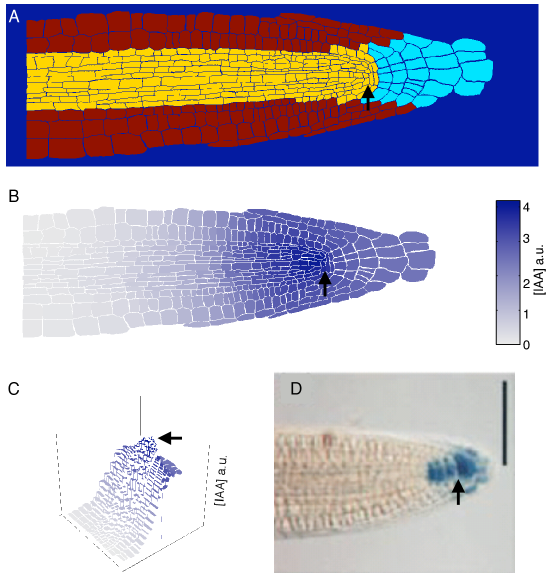
Figure 10: Root simulations from a manually traced Arabidopsis specimen from Swarup et al. [34, Fig. 1]. (A) Traced root used for the simulation. Cell size was determined by computing the area; neighbor relations and interface area were obtained by computing the length of a shared boundary. Diffusion coefficients and per-cell hormone production are the same for all cells. (B,C) Result of simulation. Note the predicted peak of concentration (arrows). (D) Stained root from Casimiro et al. [6, Fig.1A] showing a peak at the tip (arrow). Our model predicts this peak even though all parameters are kept uniform.

4 Numerical Simulations

4.1 Background

Here we provide background definitions and results separated in two major categories: geometry and graph theory. The first category is needed to prove the results about the steady-state of certain dynamical processes, and the second category is used to prove that a discretization of these processes is well behaved.

A graph $G=(V,E)$ is a combinatorial structure that consists of three things: a set of vertices (or nodes) $V$, a set of edges $E$, and an incidence relation. The edges describe which vertices are connected and the incidence relation attributes an order to each connection. For example, the edge $e=(i,j)$ says that node $i$ is connected to node $j$ and that it “starts” at $i$ and “ends” at $j$. The number of edges of which vertex $j$ is an end is called the degree of $i$. Each edge may take a value, called a weight, and these values can be recorded in an adjacency matrix $A$ of size $n\times n$ where $n=|V|$. So, $A_{ij}$ is the value for the edge $(i,j)$. Note that the matrix will be symmetric if the direction of the edges does not matter, i.e. $A_{ij}=A_{ji}$. This is the undirected case, which will be discussed in this paper and describes the (Helmholtz) dynamics of auxin concentration. In the following paper [13], however, directed graphs will be needed and $A_{ij}=-A_{ji}$ in some cases.

A matrix can be described by its eigenvectors and eigenvalues. A vector $v$ is called an eigenvector (or characteristic vector) of the matrix $A$ iff $Av=\lambda v$ for some number $\lambda$, which is the corresponding eigenvalue (or characteristic value).

The graph Laplacian $L(G)$ of a graph $G$ is given by $L(G)=D(G)-A(G)$ where $D$ is the diagonal degree matrix ($D_{ii}=$degree of $i$) and $A$ is the adjacency matrix. The following is a standard result (e.g. see [4]).

Theorem 27.

Let $G$ be a connected graph on $n$ vertices and denote by $\lambda_{0}\leq\lambda_{1}\leq\cdots\leq\lambda_{n-1}$ the eigenvecotrs of $L=L(G)$, the graph Laplacian. Then:

1. All $\lambda_{i}$ are real;

2. $\lambda_{0}=0$, with eigenvector $\mathbf{1}=[1,1,\cdots,1]^{T}$;

3. $\lambda_{1}>0$; and

4. the eigenvectors of $L$ span $\mathbb{R}^{n}$.

A matrix $A$ is called positive definite if $v^{t}Av>0$ (where $v^{t}$ is the transpose of $v$) for all non-zero vectors $v$, and it is semi-definite if some non-zero vector $w$ exists such that $v^{t}Av=0$. Note that $L(G)$ is positive semi-definite.

The determinant of an $n\times n$ matrix $A$ is given by the following formula:

$$det(A)=\sum_{\sigma\in S_{n}}sgn(\sigma)\prod_{i=1}^{n}A_{i,\sigma(i)}$$

where $\sigma$ is a permutation on $n$ elements and $sgn(\sigma)$ is the sign of the permutation: positive if the permutation can be produced by an even number of element exchanges and negative otherwise. A matrix $A$ is invertible – i.e. $A^{-1}$ exists such that $A^{-1}A=Id$ – iff $det(A)\neq 0$. The determinant is equal to the product of eigenvalues, $det(A)=\prod_{i}\lambda_{i}$, so $L(G)$ is not invertible.

4.2 Discrete Simulations

In this section we prove that appropriate discretizations of the continuous equations may be solved numerically. Specifically, we show that Eq. 1 and Eq. 5 converge to a unique solution as $t\to\infty$ and show how to obtain this solution without iteration. We shall not assume anything about the dimensionality of the space which contains the cells, only that they are connected.

Suppose there are $n$ cells in a conglomerate $\Omega$ where each cell shares an interface with at least one other cell and that the conglomerate is connected in this fashion. Labeling each cell with a number from 1 to $n$, suppose that each cell $i$ contains a hormone at concentration $c(i)$. The interfaces allow this hormone to diffuse following Fick’s law, so assuming the diffusion constant through an interface between cell $i$ and cell $j$ is $D_{ij}$, then the flow into cell $i$ through each existing interface is given by $D_{ij}(c(j)-c(i))$. Thus, the diffusion of the hormone through the conglomerate may be described by a matrix $-L$ applied to the vector $\mathbf{c}$ of concentrations, where

$$-L_{ij}=\left\{\begin{array}[]{l@{\hspace{1em}}r}D_{ij}\hfil\hskip 10.00002pt&i\neq j\\ -\sum_{j\neq i}D_{ij}\hfil\hskip 10.00002pt&i=j\end{array}\right.$$

Notice that $L$ is the graph Laplacian for the graph where each cell is a node and the edge weights are the diffusion coefficients $D_{ij}$.

Now suppose that the hormone concentration in cell $i$ is somehow maintained at a fixed level $c(i)=c_{f}$; refer to such a cell as a sink. Then the diffusion process in or out of cell $i$ has no effect on its concentration $c(i)$, but neighboring cells $c(j)$ will be affected by $c(i)$. Hence, the new matrix $M_{ij}$ describing the diffusion process looks exactly like $-L$ except for the rows corresponding to sinks; if $i$ is a sink then $M_{ii}=1$ and $M_{ij}=0$ for $j\neq i$. This means that $det(M)=det(M^{ns})$, and that $M$ is no longer symmetric, because any neighbor $j$ of $i$ which is not a sink will induce $M_{ji}=D_{ji}$. However, the sub-matrix $M^{ns}$ of $M$ with rows and columns corresponding to all cells which are not sinks is symmetric. In fact, the next lemma follows immediately.

Lemma 28.

Let $\Omega$ be a conglomerate of $n=n_{s}+n_{r}$ cells of which $n_{s}$ are sinks. Label the sinks 1 to $n_{s}$ and the rest with $n_{s}+1$ to $n$. Let $M^{ns}=M(n_{s}+1:n,n_{s}+1:n)$ be the $n_{r}\times n_{r}$ sub-matrix and $-L$ be the graph Laplacian of the sub-graph $G^{(ns)}$ of non-sink cells. Let $C_{ij}$ by an $n_{r}\times n_{r}$ diagonal matrix such that for each cell $i$ in $G^{(ns)}$ neighboring sinks $s_{j}$ we have $C_{ii}=\sum_{s_{j}}D_{is_{j}}$. Then, for a suitable labeling,

$$M^{ns}=-L-C~{}.$$

If we also assume that the hormone is destroyed in each non-sink cell $i$ at a rate proportional to the concentration in cell $i$, then the sub-matrix becomes

$$M^{ns}=-L-C-\alpha I~{}$$ (7)

where $I$ is the $n_{r}\times n_{r}$ identity matrix. Observe that $M$ is invertible if and only if $M^{ns}$ is invertible because $det(M)=det(M^{ns})$.

Lemma 29.

If either $\alpha>0$ or $\alpha\geq 0$ and there is at least one sink cell, then the matrix $M$ is invertible and has strictly negative eigenvalues.

Proof.

As observed above, it suffices to show that $det(M^{ns})\neq 0$. We shall use the following result and apply it to $-M^{ns}$ from Eq. 7.

Lemma 30.

Let $D=\left\{{d_{ij}}\right\}$ be an $n\times n$ diagonal matrix with $d_{ii}\geq 0$ with at least one $d_{ii}>0$. Let $L$ be the graph Laplacian of a connected graph on $n$ vertices. Then $M=L+D$ is symmetric positive definite. It follows that $M$ is invertible and has strictly positive eigenvalues.

Proof.

From Theorem 27 we see that $L$ is positive semi-definite. So, if $\mathbf{v}\in\mathbb{R}^{n}$ and $\mathbf{v}\neq 0$, then $\mathbf{v}^{T}L\mathbf{v}\geq 0$ with equality reached only for $\mathbf{v}=s\mathbf{1}$ where $s\neq 0$. Similarly, $D$ is positive semi-definite because $\mathbf{v}^{T}D\mathbf{v}=\sum_{i}d_{ii}v_{i}^{2}$ and all terms are non-negative. Further, $(s\mathbf{1})^{T}D(s\mathbf{1})=\sum_{i}d_{ii}s^{2}>0$ since $s^{2}>0$ and at least one entry in $D$ is strictly positive. Finally, if $\mathbf{v}\in\mathbb{R}^{n}$ and $\mathbf{v}\neq 0$, then

$$\mathbf{v}^{T}M\mathbf{v}=\mathbf{v}^{T}(L+D)\mathbf{v}=\mathbf{v}^{T}L\mathbf{v}+\mathbf{v}^{T}D\mathbf{v}>0~{}.$$

This finishes the proof of Lemma 30. ∎

Now, let $D=C+\alpha I$. If there is at least one sink, then at least one $C_{ii}>0$; if $\alpha>0$ then all $D_{ii}>0$. Hence Lemma 30 applies and completes the proof of Lemma 29. ∎

To complete the discretization of the continuous process, suppose that $\rho_{\Omega}(i)=K/S(i)$, with units ($mass*time^{-1}*volume^{-1}$), is the rate at which cell $i$ produces the hormone. Setting $S(i)$ to be the size of cell $i$, we obtain the following discrete dynamics:

$$\mathbf{c}^{(t+\Delta t)}=\mathbf{c}^{(t)}+\Delta t\underbrace{\left({M\mathbf{c}^{(t)}+\rho_{\Omega}}\right)}_{dc/dt}$$ (8)

where $\Delta t$ is the time step. We wish to show that, given a small enough $\Delta t$, $\mathbf{c}$ will converge to a unique value.

Observe that the update rule in Eq. 8 may represented as $\tilde{}\mathbf{c}^{(t+\Delta t)}=U\tilde{}\mathbf{c}^{(t)}$ by writing

$$\underbrace{\left({\begin{array}[]{c}c^{(t+\Delta t)}(1)\\ c^{(t+\Delta t)}(2)\\ \vdots\\ c^{(t+\Delta t)}(n)\\ 1\end{array}}\right)}_{\tilde{}\mathbf{c}^{(t+\Delta t)}}=\underbrace{\left[\begin{array}[]{cc}\left[\begin{array}[]{ccccc}\\ &(\Delta t)M+I&\\ \\ \\ \end{array}\right]&\begin{array}[]{c}\Delta t{\rho_{\Omega}}(1)\\ \Delta t{\rho_{\Omega}}(2)\\ \vdots\\ \Delta t{\rho_{\Omega}}(n)\end{array}\\ 0&1\end{array}\right]}_{U}\underbrace{\left({\begin{array}[]{c}c^{(t)}(1)\\ c^{(t)}(2)\\ \vdots\\ c^{(t)}(n)\\ 1\end{array}}\right)}_{\tilde{}\mathbf{c}^{(t)}}$$

where $I$ is the $n\times n$ identity matrix. The convergence of the process now reduces to showing that $U^{k}\tilde{}\mathbf{c}^{(0)}$ converges as $k\to\infty$. Notice that $U$ has the block form of the following three matrices

$$U_{a}=\left[\begin{array}[]{cc}A&\mathbf{v}_{a}\\ \mathbf{0}&1\end{array}\right],\quad U_{b}=\left[\begin{array}[]{cc}B&\mathbf{v}_{b}\\ \mathbf{0}&1\end{array}\right],\quad U_{c}=\left[\begin{array}[]{cc}C&\mathbf{v}_{c}\\ \mathbf{0}&1\end{array}\right]$$

where $A$, $B$ and $C$ are $n\times n$ matrices; $\mathbf{v}_{a}$, $\mathbf{v}_{b}$ and $\mathbf{v}_{c}$ are $n\times 1$ vectors; and $\mathbf{0}$ is a $1\times n$ vector. The product of two such matrices preserves the block form; e.g. $U_{c}=U_{a}U_{b}$ by setting $C=AB$ and $\mathbf{v}_{c}=A\mathbf{v}_{b}+\mathbf{v}_{a}$. Therefore, by induction on $k$, the blocks of $U_{c}=U_{a}^{k}$ must be $C=A^{k}$ and $\mathbf{v}_{c}=\sum_{i=0}^{n-1}A^{i}\mathbf{v}_{a}$.

Theorem 31.

Suppose that each cell $i$ has size $S(i)$, produces a hormone at a rate $\rho_{\Omega}(i)$ and destroys the hormone at a rate $\alpha c(i)$ with $\alpha\geq 0$. If $\alpha>0$ or there is at least one sink cell, then for a sufficiently small $\Delta t$ the discrete process in Eq. 8 will converge to $\mathbf{c}^{*}=-M^{-1}(\rho_{\Omega}/S)$.

Proof.

The conditions of Lemma 29 apply, so $M$ has strictly negative eigenvalues and $M^{-1}$ exists. Choose $0<\Delta t<1/\lambda$ where $\lambda$ is the largest (in absolute value) eigenvalue of $M$. Thus $A=\Delta tM+I$ will have eigenvalues $0<\left|{\lambda_{i}}\right|<1$; it follows that $\lim_{k=\infty}A^{k}=0$. Now, from the above, $\mathbf{v}_{c}=\sum_{i=0}^{k-1}A^{i}\mathbf{v}_{a}=(A^{k}-I)(A-I)^{-1}\mathbf{v}_{a}=(A^{k}-I)(\Delta tM)^{-1}\mathbf{v}_{a}$ and the claim follows. ∎

This result demonstrates that an iterative process will indeed converge—assuming perfect arithmetic operations—but it also shows that the equilibrium can be computed much more efficiently. It suffices to solve the linear system $\mathbf{c}^{*}=-M^{-1}(\rho_{\Omega}/S)$. The system is well behaved numerically whenever $\alpha$ is sufficiently large, because the condition number of this matrix is roughly equal to the largest degree of the graph, times $D$ divided by $\alpha$; see Dahlquist and Björck [9] for a discussion of matrix condition numbers.

4.3 Geometric Domain Definition

In this section we outline how the domains—representing leaves, roots, etc.—are defined geometrically and then converted into the graph representation discussed in the previous section. Ultimately, the geometry of the domains should correspond to and be comparable to the geometry of real plant tissues. Thus, we define the domains by manipulating images of those tissues. Both the cell size and the cell neighbors (i.e. the topology of the graph) are computed from an image.

In this paper we adopted a pixel-based approach whereby the organ is drawn as a digital image and the color of each pixel encodes some information: whether the pixel is part of the domain or not, the value of the production function $\rho$, whether the pixel is a sink or part of the vein pattern, etc. The natural connectivity of pixels on a square grid—four or eight neighbors—then defines the topology of the graph. The final diffusion matrix is built after defining the diffusion constants for each pair of pixel colors.

But this representation also allows us to define a cell by using multiple pixels. Fig. 9 shows an example in which a cell consists of several black pixels—representing the interior—surrounded by green pixels—representing the cell walls. None produce auxin except for a single dark-green pixel in the middle of the interior pixels. Thus, each cell produces auxin at the same rate (the rate of the center pixel) but cells may have different sizes. Moreover, the diffusion coefficient in the interior of the cell may be different from the diffusion coefficient through the cell wall. Our usual assumption is that the interior diffusion coefficient is much larger.

5 Conclusion

We have developed the foundations for a theory of how global information about shape is related to the distance transform, and how several of the essential properties of this distance transform can be computed by a simple reaction-diffusion equation. The model has its roots in our earlier Constant Production Hypothesis, and is based on a computational abstraction that all cells behave according to the same rules. Most importantly, it provides a mechanism that illustrates how “hot spots” of concentration can develop from structural conditions rather than differential production induced by an explicit developmental program.

The explicit assumption about hormone depletion—the Proportional Destruction Hypothesis—greatly increased the scope of our earlier model [15]. We showed that there are at least two additional ways in which a distance map becomes locally available to a group of cells, and that testable predictions ensue. And although the available data is insufficient to compare the predictions to the actual numbers, the qualitative trend is accurately reproduced and explicit measurements are suggested by updated model. The analysis and assumptions of Section 3.4, in effect, describe further experiments to test the theory.

The simulations in this paper, which involved detailed anatomical considerations, show the power of such calculations. That an auxin concentration peak emerged properly near the root tip illustrates their role is sufficency rather than necessity.

Nevertheless, our model is still too abstract to be deemed biological. In particular, it is well known that diffusion is not the only transport mechanism responsible for auxin flow. Active, or at least facilitated, transport carriers are known to exist, which our current formulation does not consider. That is a topic of our companion paper. For now, we remark that the Fickian transport and reaction diffusion equation developed here can provide an abstraction in such a manner that its main properties hold when more detailed facilitated transport is taken into account.

References

- [1] M. Abramowitz and I. A. Stegun. Handbook of Mathematical Functions. Dover, 1972.
- [2] R. P. Bhalerao, J. Eklöf, K. Ljung, A. Marchant, M. Bennett, and G. Sandberg. Shoot-derived auxin is essential for early lateral root emergence in arabidopsis seedlings. The Plant Journal, 29:325–332, 2002.
- [3] H. Blum. Biological shape and visual science (part 1). Journal of Theoretical Biology, 38:205–287, 1973.
- [4] N. Briggs. Algebraic Graph Theory. Cambridge University Press, 2 edition, 1993.
- [5] L. Calabi and W. E. Hartnett. Shape recognition, prairie fires, convex deficiencies and skeletons. The American Mathematical Monthly, 75(4):335–342, April 1968.
- [6] I. Casimiro, A. Marchant, R. P. Bhalerao, T. Beeckman, S. Dhooged, R. Swarup, N. Graham, D. Inzé, G. Sandberg, P. J. Casero, and M. Bennett. Auxin transport promotes arabidopsis lateral root initiation. The Plant Cell, 13:843–852, 2001.
- [7] H. I. Choi, S. W. Choi, and H. P. Moon. Mathematical theory of medial axis transform. Pacific Journal of Mathematics, 181(1):57–88, November 1997.
- [8] R. Courant and D. Hilbert. Methods of mathematical physics, volume 2. Interscience, 1962.
- [9] G. Dahlquist and Ȧ. Björck. Numerical Methods. Dover, 2003.
- [10] N. Dharmasiri, S. Dharmasiri, and M. Estelle. The F-box protein TIR1 is an auxin receptor. Nature, 435:441–445, 2005.
- [11] P. Dimitrov, J. Damon, and K. Siddiqi. Flux invariants for shape. In Computer Vision and Pattern Recognition, 2003, volume I, pages I–835, 2003.
- [12] P. Dimitrov and S. W. Zucker. Patterns in plant development #1: Uniform production and proportional destruction of auxin. submitted to PLoS.
- [13] P. Dimitrov and S. W. Zucker. Patterns in plant development #2: Facilitated transport and uniform gradient. submitted to PLoS.
- [14] P. Dimitrov and S. W. Zucker. Patterns in plant development #3: Early pin patterning and shoot-root synchronization. submitted to PLoS.
- [15] P. Dimitrov and S. W. Zucker. A constant production hypothesis that predicts the dynamics of leaf venation patterning. Proc. Natl. Acad. Sci USA, 103:9363–9368, 2006.
- [16] P. Dimitrov and S. W. Zucker. Tech report – proof. Technical Report 1345, Computer Science, Yale University, 2006. ftp://ftp.cs.yale.edu/pub/TR/tr1345.pdf.
- [17] H. Federer. Curvature measures. Trans. Amer. Math. Soc., 93:418–491, 1959.
- [18] A. Gierer and H. Meinhardt. A theory of biological pattern formation. Kybernetik, 12:30–39, 1972.
- [19] D. Gilbarg and N. S. Trudinger. Elliptic Partial Differential Equations of Second Order. Springer-Verlag, 1983.
- [20] L. G. Harrison. Kinetic Theory of Living Pattern. Cambridge University Press, 1993.
- [21] L. Kannenberg. Uniqueness of solutions to helmholtz’s equation with linear boundary conditions. Am. J. Phys., 57(1):60–63, January 1989.
- [22] S. Kepinski and O. Leyser. The Arabidopsis F-box protein TIR1 is an auxin receptor. Nature, 435:446–451, 2005.
- [23] S. G. Krantz and H. R. Parks. Distance to hypersurfaces. J. Differential Equations, 40(1):116–120, 1981.
- [24] K. Ljung, R. P. Bhalerao, and G. Sandberg. Sites and homeostatic control of auxin biosynthesis in arabidopsis during vegetative growth. The Plant Journal, 28(4):465–474, 2001.
- [25] J. N. Mather. Distance from a submanifold in euclidean space. Proceedings of Symposia in Pure Mathematics, 40(2), 1983.
- [26] G. Matheron. Examples of Topological Properties of Skeletons, volume 2 of Image Analysis and Mathematical Morphology, chapter 11, pages 217–238. Academic Press, 1988.
- [27] T. Nelson and N. Dengler. Leaf vascular pattern formation. The Plant Cell, 9:1121–1135, 1997.
- [28] T. R. Pray. Foliar venation of angiosperms. II. histogenesis of the venation of liriodendron. American Journal of Botany, 42(1):18–27, 1955.
- [29] P. H. Raven, R. F. Evert, and H. Curtis. Biology of Plants. Worth Publishers, Inc., third edition, 1981.
- [30] F. B. Salisbury and C. W. Ross. Plant Physiology. Wadsworth Publishing Company, fourth edition, 1992.
- [31] E. Scarpella, P. Francis, and T. Berleth. Stage-specific markers define early steps of procambium development in arabidopsisleaves and correlate termination of vein formation with mesophyll differentiation. Development, 131:3445–3455, 2004.
- [32] E. Scarpella, D. Marcos, J. Friml, and T. Berleth. Control of leaf vascular patterning by polar auxin transport. Genes and Development, 20(8):1015–1027, 2006.
- [33] K. Siddiqi, S. Bouix, A. R. Tannenbaum, and S. W. Zucker. Hamilton-jacobi skeletons. International Journal of Computer Vision, 48:215, 2002.
- [34] R. Swarup, J. Friml, A. Marchant, K. Ljung, G. Sandberg, K. Palme, and M. Bennett. Localization of the auxin permease aux1 suggests two functionally distinct hormone transport pathways operate in the arabidopsis root apex. Genes and Developlment, 15:2648–2653, 2001.
- [35] W. D. Teale, I. A. Paponov, and K. Palme. Auxin in action: signalling, transport and the control of plant growth and development. Nature Reviews Molecular Cell Biology, 7:847–859, 2006.
- [36] H. Tsukaya. Leaf development. In C. R. Somerville and E. M. Meyerowitz, editors, The Arabidopsis Book. American Society of Plant Biologists, 2002.
- [37] A. M. Turing. The chemical basis of morphogenesis. Philosophical Transactions of the Royal Society of London B, 237:37–72, 1952.
- [38] H. Vöchting. Ueber theilbarkeit im pflanzenreich und die wirkung innerer und äusserer krafte auf organbildung an pflanzentheilen. Pfüger’s Arch., 15:153–190, 1877.
- [39] H. Vöchting. Ueber Organbildung im Pflanzenreich, volume 1. Max Cohen & Sohn, Bonn, Germany, 1878.
- [40] F. W. Warner. Foundations of Differntiable Manifolds and Lie Groups. GTM 94. Springer, 1983.
- [41] L. Wolpert. Positional information and the spatial pattern of cellular differentiation. Journal of Theoretical Biology, 25:1–47, 1969.
- [42] L. Wolpert. Positional information and pattern formation. Phil. trans. R. Soc. Lond. B, 295:441–450, 1981.