Microlensing variability in FBQ 0951+2635: short-timescale events or a long-timescale fluctuation?

Abstract

We present and analyse new $R$-band frames of the gravitationally lensed double quasar FBQ 0951+2635. These images were obtained with the 1.5m AZT-22 Telescope at Maidanak (Uzbekistan) in the 2001$-$2006 period. Previous results in the $R$ band (1999$-$2001 period) and the new data allow us to discuss the dominant kind of microlensing variability in FBQ 0951+2635. The time evolution of the flux ratio $A/B$ does not favour the continuous production of short-timescale ($\sim$ months) flares in the faintest quasar component B (crossing the central region of the lensing galaxy). Instead of a rapid variability scenario, the observations are consistent with the existence of a long-timescale fluctuation. The flux ratio shows a bump in the 2003$-$2004 period and a quasi-flat trend in more recent epochs. Apart from the global behaviour of $A/B$, we study the intra-year variability over the first semester of 2004, which is reasonably well sampled. Short-timescale microlensing is not detected in that period. Additional data in the $i$ band (from new $i$-band images taken in 2007 with the 2m Liverpool Robotic Telescope at La Palma, Canary Islands) also indicate the absence of short-timescale events in 2007.

1 Introduction

FBQ 0951+2635 was discovered a decade ago by Schechter et al. (1998). This is a double quasar (consisting of two components A and B) at redshift $z_{s}$ = 1.246, which is gravitationally lensed by an early-type galaxy at $z_{l}$ = 0.260 (Eigenbrod et al., 2007). The main lensing galaxy probably belongs to a group of galaxies at similar redshift (Williams et al., 2006).

Table 1: New optical observations of FBQ 0951+2635.

Observatory	Telescope	Camera	Filter	Period	Nights	Exposures/night
Maidanak (Uzbekistan)	1.5m AZT-22	BroCam	$R$	April 2001	1	2 (120 + 180 s)
				March 2002	3	2$-$4 (180/240 s)
				Apr-May 2003	2	2 (180 s)
				Jan-May 2004	14	3$-$5 (180/210 s)
				Dec 2004-Apr 2005	6	4$-$8 (180 s)
				Nov-Dec 2005	3	2 (300 s)
				Apr-May 2006	8	10 (180 s)
La Palma (Canary Islands)	2m Liverpool	RATCam	$i$	Feb-May 2007	52	5 (100 s)

Optical follow-up of FBQ 0951+2635 has been done in the current decade. This includes early imaging and monitoring with the HST (Kochanek et al., 2000) and the Nordic Optical Telescope (NOT, Jakobsson et al., 2005), as well as imaging from the Sloan Digital Sky Survey (SDSS, Adelman-McCarthy et al., 2008). The 2.5-year monitoring campaign at the NOT focused on the $R$ passband. These $R$-band frames allowed Jakobsson et al. (2005) and Paraficz et al. (2006) to study the time delay between components and early extrinsic variability. The time delay between A and B is of about two weeks (Jakobsson et al., 2005), and there is clear evidence for $R$-band extrinsic variations in the 1999$-$2001 period (Paraficz et al., 2006). Paraficz et al. (2006) showed a possible gradient of about 0.1 mmag day^-1, as well as a possible 50-mmag event on a timescale of several months. These extrinsic fluctuations (which are not originated in the source quasar) were attributed to microlensing by collapsed objects within the lensing galaxy (e.g., Wambsganss, 1990, and references therein).

However, the information obtained in the first years of monitoring with the NOT (1999$-$2001) does not permit to decide on the true microlensing variability, so additional imaging is required to address this issue. For example, in Fig. 2 (middle and bottom panels) of Paraficz et al. (2006), one sees that the microlensing gradients can account for basically all variability without the need of introducing additional short-term ($\sim$ months) microlensing events (see the distributions of points around the linear fits). Alternatively, in the same panels of Fig. 2 of Paraficz et al. (2006), sets of short-term microlensing events can also explain the observed variations. Thus, it is unclear what kind of microlensing fluctuations occur in FBQ 0951+2635: short-timescale events or gradients lasting years (tracing a long-timescale event)?. Although both kinds of fluctuations may be present, one reasonably expects the presence of a dominant kind accounting for most of the observed microlensing variability. In this paper, we try to identify the dominant microlensing variations.

In Sect. 2 we analyse new $R$-band images taken at the Maidanak Observatory in the 2001$-$2006 period. The previous NOT results and the Maidanak analysis permit us to check the kind of microlensing fluctuations in the red part of the optical continuum (in the observer frame). In Sect. 3 we study FBQ 0951+2635 by using a redder optical filter ($i$ Sloan passband). The $i$-band frames correspond to a new monitoring campaign with the 2m Liverpool Robotic Telescope (LRT) during the first semester of 2007. To support our main results, we also use a few complementary frames in public and private archives. The conclusions are presented in Sect. 4.

2 Light curve and flux ratio in the $R$ band

FBQ 0951+2635 is part of a compact lens system, since the two quasar components are separated by 1$\aas@@fstack{\prime\prime}$1 (Schechter et al., 1998) and the very faint lensing galaxy is 0$\aas@@fstack{\prime\prime}$2 away from the faintest component B (Jakobsson et al., 2005). Fortunately, the lensing galaxy remains too faint to be detected with a standard $R$ filter (Jakobsson et al., 2005), and this is an advantage when doing photometry. Thus, the system can be described by two stellar-like objects. There are two field stars near the lensed quasar: the bright star S1 and the faint star S3 (see Fig. 1). The FWHM of the seeing disc is measured on the S1 star, which is also used to estimate the point spread function (PSF) of the stellar-like sources. This estimation allows us to obtain PSF fitting photometry for the double quasar.

A single-epoch magnitude difference ($m_{B}-m_{A}$) could not represent the magnitude difference at the same emission time ($\Delta m_{BA}$), because one should take into account the 16-day time delay between components (Jakobsson et al., 2005). However, the typical variability of FBQ 0951+2635 on a timescale of $\sim$ 2 weeks gives us the typical amplitude of the deviations $\delta=m_{B}-m_{A}-\Delta m_{BA}$, so a correction for simultaneity can be estimated from variability studies. Throughout most of this paper, we derive $\Delta m_{BA}$ values from single-epoch magnitude differences, whose photometric uncertainties are properly enlarged to incorporate the simultaneity error $\sigma_{sim}$ (i.e., the typical amplitude of $\delta$). We adopt $\sigma_{sim}$ = 0.03 mag, which is consistent with the $R$-band root-mean-square (rms) variability of FBQ 0951+2635 over a 16-day period (see details in subsection 2.1), as well as with the $i$-band variability over such timescale (see subsection 3.1). All single-epoch measurements of $\Delta m_{BA}$ include the 0.03-mag uncertainty added in quadrature to the photometric errors. The flux ratio between components is given by $A/B=10^{0.4\times\Delta m_{BA}}$.

2.1 Maidanak follow-up observations

The Maidanak gravitational lens monitoring programme is being conducted by an international collaboration of astronomers from Russia, Ukraine, Uzbekistan, and other countries. The median FWHM ($\sim$ 0$\aas@@fstack{\prime\prime}$7) and number of clear nights ($\sim$ 200 nights per year) at Mt. Maidanak (Artamonov et al., 1987; Ehgamberdiev et al., 2000) permit to obtain high-resolution images of compact lens systems (e.g., Koptelova et al., 2005), and here we present and analyse $R$-band observations of FBQ 0951+2635. These Maidanak homogeneous observations from April 2001 to May 2006 are an important tool to understand the microlensing variability in the double quasar.

Our Maidanak monitoring consisted of 190 frames (exposures) in the $R$ band, which were taken with the 1.5m AZT-22 Telescope at Mt. Maidanak (Uzbekistan) on 37 different nights (see Table 1). We used the LN2-cooled CCD camera (BroCam) with SITe ST-00A CCD chip. This 2000$\times$800 CCD detector has pixels with a physical size of 15 $\mu$m, giving angular scales of 0$\aas@@fstack{\prime\prime}$135 pixel^-1 (long-focus mode) and 0$\aas@@fstack{\prime\prime}$268 pixel^-1 (short-focus mode). The gain and readout noise are 1.2 e^- ADU^-1 and 5.3 e^-, respectively.

Table 2: $R$-band photometry of FBQ 0951+2635 from 2001 to 2006.

(1)	(2)	(3)	(4)	(5)	(6)	(7)	(8)	(9)	(10)	(11)	(12)	(13)	(14)	(15)
10415	2	904.073	150	0.94	0.03	56.0	16.884	0.001	17.948	0.015	1.063	0.033	19.490	0.013
20304	4	1237.797	180	0.96	0.05	53.0	16.990	0.008	18.056	0.030	1.065	0.048	19.462	0.012
20311	2	1244.790	240	0.99	0.19	53.0	16.987	0.003	18.098	0.039	1.111	0.052	19.469	0.004
20314	2	1247.782	180	0.89	0.10	53.0	16.995	0.005	18.104	0.012	1.108	0.031	19.448	0.035
30427	2	1656.661	180	1.06	0.12	38.0	16.995	0.000	18.271	0.009	1.276	0.031	19.458	0.030
30521	2	1680.656	180	0.89	0.08	27.0	17.028	0.000	18.210	0.014	1.182	0.033	19.406	0.056
40116	3	1920.994	180	1.04	0.06	64.0	17.055	0.011	18.266	0.026	1.212	0.048	19.464	0.035
40122	4	1926.879	180	0.91	0.11	81.0	17.062	0.003	18.306	0.007	1.244	0.031	19.455	0.011
40209	5	1944.849	180	0.97	0.05	40.0	17.072	0.002	18.296	0.014	1.224	0.033	19.474	0.014
40213	4	1948.907	210	1.00	0.13	62.5	17.047	0.005	18.304	0.009	1.257	0.033	19.462	0.008
40219	4	1954.904	180	0.99	0.19	74.5	17.021	0.004	18.346	0.009	1.325	0.031	19.460	0.012
40222	4	1957.851	180	1.01	0.17	44.5	17.038	0.002	18.328	0.018	1.289	0.036	19.467	0.026
40226	4	1961.877	180	1.05	0.10	29.0	17.059	0.006	18.365	0.013	1.306	0.035	19.483	0.022
40227	4	1962.868	180	0.91	0.09	80.5	17.036	0.003	18.330	0.009	1.294	0.031	19.439	0.007
40301	4	1965.876	180	0.93	0.20	44.0	17.046	0.002	18.333	0.013	1.287	0.033	19.455	0.013
40409	3	2004.748	180	1.13	0.11	63.3	17.092	0.008	18.207	0.017	1.115	0.038	19.483	0.013
40413	4	2012.684	180	0.93	0.05	69.0	17.097	0.001	18.295	0.005	1.198	0.030	19.488	0.020
40504	4	2029.677	180	0.97	0.05	24.5	17.100	0.006	18.327	0.011	1.227	0.034	19.504	0.016
40511	4	2036.671	180	0.99	0.08	63.5	17.068	0.005	18.337	0.009	1.270	0.033	19.444	0.012
40520	3	2045.693	180	1.04	0.04	60.0	17.078	0.004	18.302	0.009	1.225	0.032	19.448	0.007
41204	6	2243.062	180	0.90	0.09	24.3	17.208	0.005	18.446	0.010	1.239	0.031	19.480	0.029
41205	8	2243.983	180	0.89	0.14	22.8	17.217	0.004	18.448	0.012	1.231	0.032	19.479	0.012
50208	6	2309.834	180	0.88	0.06	62.0	17.241	0.003	18.469	0.007	1.228	0.031	19.473	0.008
50214	6	2315.840	180	0.97	0.05	62.3	17.226	0.003	18.430	0.012	1.205	0.033	19.475	0.013
50306	6	2335.815	180	0.97	0.03	50.0	17.251	0.004	18.481	0.006	1.231	0.031	19.478	0.016
50414	4	2374.726	180	0.90	0.04	47.5	17.236	0.006	18.459	0.007	1.224	0.032	19.430	0.006
51126	2	2601.018	300	1.09	0.03	65.0	17.339	0.014	18.488	0.015	1.150	0.041	19.489	0.017
51128	2	2602.974	300	0.92	0.09	79.0	17.322	0.003	18.569	0.019	1.247	0.034	19.420	0.010
51201	2	2606.027	300	0.90	0.10	61.0	17.337	0.002	18.576	0.002	1.239	0.030	19.438	0.003
60402	10	2727.786	180	0.83	0.15	80.2	17.372	0.002	18.649	0.005	1.278	0.030	19.377	0.006
60411	10	2736.793	180	1.11	0.15	28.4	17.511	0.017	18.457	0.036	0.946	0.060	19.481	0.017
60413	10	2738.767	180	1.06	0.08	29.0	17.433	0.006	18.588	0.024	1.155	0.042	19.423	0.024
60417	10	2742.703	180	1.05	0.13	82.0	17.428	0.003	18.610	0.007	1.182	0.031	19.401	0.005
60509	10	2764.678	180	1.04	0.17	38.6	17.451	0.003	18.637	0.011	1.185	0.032	19.429	0.011
60511	10	2766.681	180	1.17	0.10	38.2	17.529	0.019	18.422	0.043	0.893	0.069	19.437	0.014
60514	10	2769.706	180	0.97	0.16	26.2	17.483	0.009	18.682	0.012	1.198	0.032	19.453	0.024
60517	10	2772.664	180	1.14	0.09	56.6	17.472	0.004	18.528	0.011	1.055	0.033	19.416	0.011

(1) civil date (ymmdd), (2) number of frames, (3) JD$-$2451100, (4) exposure time per frame (s), (5) FWHM of the seeing disc (″), (6) ellipticity of the seeing disc, (7) SNR of an 18 mag star (within a 2″ aperture radius), (8) flux of A (mag), (9) error in flux of A (mag), (10) flux of B (mag), (11) error in flux of B (mag), (12) $\Delta m_{BA}$ (mag), (13) error in $\Delta m_{BA}$ (mag), (14) flux of S3 (mag), and (15) error in flux of S3 (mag).

The pre-processing of each frame consists of bias subtraction, overscan trimming, flat fielding, and cosmic rays cleaning. For each observation night, we have two or more individual frames obtained under good seeing conditions: $\langle{\rm FWHM}\rangle\sim$ 1″. For example, in Fig. 1 we display the central region (1′$\times$1′) of an 180-s exposure in subarcsecond seeing conditions. This $R$-band image (logarithm of counts over the FBQ 0951+2635 field) includes the S1 star ($\sim$ 16.6 mag), the two components A and B ($\sim$ 17.1 mag and $\sim$ 18.3 mag, respectively), and the S3 star ($\sim$ 19.5 mag). Moreover, the average signal-to-noise ratio (aperture radius of 2″, i.e., $2\times$ FWHM) of an 18 mag star is $\langle{\rm SNR}\rangle\sim$ 50. Thus, most of the nightly FWHM values are less than the separation of the double quasar and there is significant signal associated with the faintest quasar component.

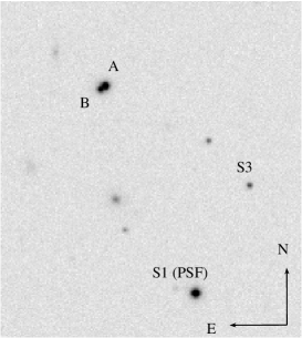
Figure 1: Central region of a Maidanak $R$-band frame of FBQ 0951+2635. This frame was taken under very good seeing conditions (FWHM = 0$\aas@@fstack{\prime\prime}$75) on January 22, 2004. The exposure time was 180 s, and we show the logarithm of counts in each pixel.

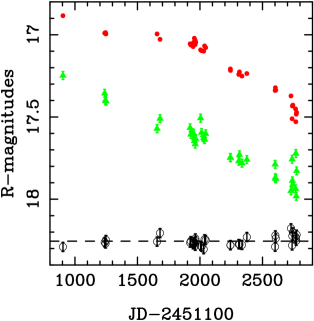
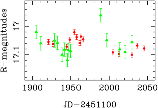
Figure 2: Maidanak $R$-band light curves of FBQ 0951+2635. Top: A (filled circles), B $-$ 0.7 mag (filled triangles), and S3 $-$ 1.2 mag (open circles). Bottom: comparison between the A fluxes in the first semester of 2004 (filled circles) and the time- and magnitude-shifted brightness record of B in that semester (filled triangles). See main text for details.

PSF fitting photometry leads to instrumental fluxes of components and field stars. These fluxes are calculated using the instrumental photometry pipeline by Shalyapin et al. (2008). We also obtain calibrated light curves (in mag) of A, B and S3, as well as single-epoch magnitude differences $m_{B}-m_{A}$. The individual values are then combined to form nightly means and standard deviations of means (i.e., standard errors). The standard errors of $m_{B}-m_{A}$ are properly enlarged because we are interested in magnitude differences at the same emission time (see explanation above). The fluxes of A, B and S3 on April 15, 2001 are also compared to the corresponding NOT fluxes at close dates (Jakobsson et al., 2005). We do not find offsets in the fluxes of A and S3, but the flux of B is slightly higher (60 mmag) than the NOT level around April 15, 2001. This offset is very probably due to a small contamination by the lens galaxy light (which is absent in the NOT fluxes), so a 60-mmag correction is taken into account when obtaining final fluxes of B. Each of the four combined curves ($m_{A}$, $m_{B}$, $m_{S3}$ and $\Delta m_{BA}$) incorporates 37 data points. These data points and other quantities of interest are presented in Table 2.

Although the standard errors may be good estimators of the nightly photometric errors in $m_{A}$, $m_{B}$ and $m_{S3}$, changes in the colour coefficient and/or the possible inhomogeneous response over the camera area could produce a substantial amount of additional noise throughout the several years of monitoring (e.g., Shalyapin et al., 2008). We check this possibility by comparing the average standard error of $m_{S3}$ and the standard deviation of $m_{S3}$ over the whole monitoring period. There is a bias factor of about $\sqrt{3}$, so we multiply the average standard errors of $m_{A}$, $m_{B}$ and $m_{S3}$ by $\sqrt{3}$ to derive typical photometric errors. These final uncertainties are 9 mmag (A), 24 mmag (B) and 28 mmag (S3). The top panel in Fig. 2 shows the final brightness records of the double quasar and the S3 star. Filled circles, filled triangles and open circles trace the behaviours of A, B (shifted by $-$0.7 mag) and S3 (shifted by $-$1.2 mag), respectively. The almost parallel fading by $\sim$ 0.6 mag of the two components indicates the presence of long-timescale intrinsic variability (extrinsic variations are discussed below). Around day 2750 (JD$-$2451100), one can see an important scatter in the light curves of A and B. This scatter was produced when the camera (BroCam) reached the end of its lifetime.

In general, sampling is unsuitable when doing analysis of short-timescale (intra-year) variability. However, this kind of study is possible in 2004 (see Table 1), i.e., around day 2000 in Fig. 2 (top panel). In the bottom panel of Fig. 2, while the filled circles describe the time evolution of the flux of A, the filled triangles represent the time- and magnitude-shifted light curve of B. The fluxes of B are advanced in 16 days (time delay; Jakobsson et al., 2005) and increased by 1.246 mag (average magnitude difference between the time-shifted record of B and the light curve of A; although bins with semi-size of 4 days are used, the average magnitude difference is within the 1.24–1.25 mag interval for any bin semi-size below 6 days). We show that there is good agreement between both brightness records, i.e., the two records are consistent with each other in the overlap periods. For this reason, we can state that short-timescale microlensing is absent or elusive. The time-delay-corrected flux ratio ($R$-band data from day 1900 to day 2050) is $A/B$ = 3.15 $\pm$ 0.05 (1$\sigma$).

We also obtain the Maidanak and NOT $R$-band typical variability of FBQ 0951+2635 at time lags $\Delta t\leq$ 100 days, with special emphasis on $\Delta t$ = 16 days, i.e., the time delay between components. The typical magnitude variation on this timescale is directly related to the simultaneity error $\sigma_{sim}$ that we introduce in the second paragraph of section 2. The rms variability $\langle(\Delta s)^{2}\rangle^{1/2}$ at lag $\Delta t$ is given by

$$\langle(\Delta s)^{2}\rangle^{1/2}=\{(1/N)\sum_{i,j}[(m_{j}-m_{i})^{2}-\sigma_{i}^{2}-\sigma_{j}^{2}]\}^{1/2},$$ (1)

where the sum only includes the ($i$,$j$) pairs verifying that $t_{j}-t_{i}\sim\Delta t$ (the number of such pairs is $N$). To derive the rms values from Eq. (1), we consider the magnitude variations in both components A and B (Maidanak fluctuations from day 2700 to day 2800 are doubtful, and thus, this Maidanak observation period is not taken into account in the analysis; see above). Fig. 3 shows the structure functions obtained from the Maidanak (filled circles) and NOT (filled squares) light curves, using independent 4-day bins. Two vertical dashed lines define the bin of interest (around the lag of 16 days). At lags $\Delta t<$ 60 days, the quasar was somewhat less active over days 50$-$1000 (NOT data). The horizontal dashed line corresponds the 0.03 mag level, which roughly coincides with the Maidanak rms variability at the lag centered on 16 days. These results explain why we take $\sigma_{sim}$ = 0.03 mag, at least at red wavelengths. We remark that the bottom panel of Fig. 2 shows a ”flare” of $\sim$ 0.1 mag over $\sim$ 10 days, between day 1990 and day 2000, and this seems to question our variability analysis in Fig. 3. However, taking the error bars into account, the true variation in the flux of B could be of about 30 mmag. This is in good agreement with the adopted variability over a 16-day period. Moreover, the $\sim$ 0.1-mag jump (considering central values) is only defined by two consecutive fluxes of the B component. In other words, it is a very poorly sampled variation in the faintest and noisest component, which is most likely caused by observational noise.

The 37 single-epoch measurements of $\Delta m_{BA}$ in Table 2 are grouped in 7 different time intervals (see the seven periods in Table 1 and the corresponding days in Table 2). We compute the weighted average and its uncertainty for each interval. These averages are then translated into 7 $R$-band flux ratio measurements with an 1$-$3% accuracy. The new flux ratio values are depicted in Fig. 4 (filled circles). For example, the flux ratio around day 2000 (3.17 $\pm$ 0.03; 1$\sigma$) is consistent with the result in two paragraphs above, which takes the time delay correction into account. Around day 2750, we obtain two estimates of $A/B$ due to the fact that the photometric data show a large scatter (see above). Firstly, we use all available nights (last open circle in Fig. 4). Secondly, only high-quality nights, i.e., FWHM $<$ 1$\aas@@fstack{\prime\prime}$1 and SNR $>$ 50, are considered (filled circle above the last open circle in Fig. 4). This second estimation seems more reliable, so the first one is assumed to be biased. We also compare the NOT flux ratio at an intermediate epoch and the corresponding Maidanak ratio from the former ST-7 CCD camera (which was operating in that epoch). The Maidanak/ST-7 1$\sigma$ measurement, 2.58 $\pm$ 0.05 (first open circle at day 484), is in excellent agreement with the NOT gradient and limits (dashed lines; see the first paragraph in subsection 2.3).

2.2 Complementary frames

A few complementary frames are used to check the reliability of the $A/B$ values from the Maidanak/BroCam homogeneous monitoring. The SDSS archive (Adelman-McCarthy et al., 2008) contains a frame of FBQ 0951+2635 in the $r$ band. This frame was taken under very good seeing conditions (FWHM = 0$\aas@@fstack{\prime\prime}$83) on December 11, 2004. From PSF fitting photometry, we infer $m_{B}-m_{A}$ = 1.22 $\pm$ 0.01 mag (1$\sigma$), which translates into $\Delta m_{BA}$ = 1.22 $\pm$ 0.03 mag and $A/B$ = 3.08 $\pm$ 0.08. The $r$-band flux of B is not corrected by a possible contamination by the lens galaxy light (the $r$-band correction will be significantly smaller than the 60-mmag offset in the $R$ band, since the $r$ Sloan filter does not transmit light at wavelengths of 700–900 nm), and the $r$-band magnitude difference is taken as the magnitude difference in the $R$ band (this is a reasonable assumption because the $r-R$ colours of both components are similar). We note the agreement between the SDSS flux ratio at day 2250 (first filled triangle in Fig. 4), and the Maidanak/BroCam value of $A/B$ around day 2300 (filled circle next to the first filled triangle in Fig. 4).

Maidanak observations in 2007 were done with the Spectral Instruments (SI) 600 Series CCD camera. It is a 4096$\times$4096, 15-$\mu$m pixel CCD. The rectangular pixels have angular scales of 0$\aas@@fstack{\prime\prime}$303 (along the horizontal axis) and 0$\aas@@fstack{\prime\prime}$258 (along the vertical axis). The camera gain is 1.45 e^- ADU^-1 and the readout noise is 4.7 e^-. These Maidanak/SI 600 Series frames belong to a private archive that is managed by several teams. To test the time evolution of $A/B$ in recent years, we use the three $R$-band frames that were taken on April 13, 2007. After applying a 60-mmag correction to the fluxes of B, the flux ratio at day 3104 is $A/B$ = 3.17 $\pm$ 0.10 (last filled triangle in Fig. 4).

2.3 Global perspective on flux ratio evolution

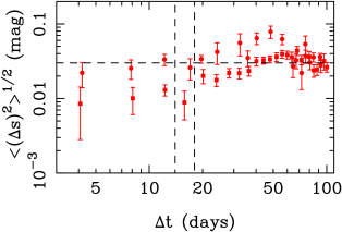
Figure 3: $R$-band rms variability at different time lags. The Maidanak (filled circles) and NOT (filled squares) trends are analysed in a separate way. We use 4-day independent bins centered on lags of 4, 8, 12, 16, 20,… days. The bin of interest (around the lag of 16 days) is highlighted from two vertical dashed lines, and the horizontal dashed line represents the 0.03 mag level.

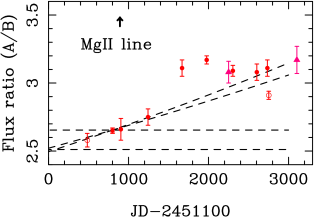
Figure 4: Time evolution of the optical continuum (red wavelengths) flux ratio of FBQ 0951+2635. We show a previous measurement from NOT $R$-band frames (filled square at day 800), as well as new Maidanak/BroCam $R$-band estimates (filled circles) and two additional results from SDSS and Maidanak/SI 600 Series frames (filled triangles). We also show the lower limit of the Mg ii flux ratio (base of the vertical arrow). The open circles and dashed lines are explained in the main text.

Paraficz et al. (2006) suggested two possible $R$-band microlensing gradients over days 50$-$1000 (see middle and bottom panels in Fig. 2 of Paraficz et al., 2006). However, the second solution (0.077 $\pm$ 0.007 mmag day^-1) seems more consistent with the analysis by Jakobsson et al. (2005), so we only consider this early microlensing slope. Jakobsson et al. (2005) found a flux ratio $A/B$ = 2.65 $\pm$ 0.02 ($\Delta m_{BA}$ = 1.06 $\pm$ 0.01 mag) when they focussed on the last part of the NOT brightness records, i.e., around day 800 (see the filled square in Fig. 4). This is fully consistent with the second linear fit by Paraficz et al. (2006) (see bottom panel in Fig. 2 of that work), which indicates $\Delta m_{BA}$ = 1.06 at day 800. Alternatively, the extrinsic variability could be due to two consecutive short-term microlensing events before day 700. While the first event was fitted to a Gaussian, it is also apparent the possible existence of a second event (see data point distribution between days 400 and 600). From day 700 to day 1000, the observations are consistent with constant microlensing because almost all error bars cross the zero level. If the two rapid events with similar amplitude are true features, no gradient is required to account for the observations. The two alternatives and their extrapolations to more recent epochs are depicted in Fig. 4. The inclined dashed lines represent the gradient of 0.077 $\pm$ 0.007 mmag day^-1 (absence of short-term events). The horizontal dashed lines are the lower and upper limits associated with the second scenario: absence of a gradient, but presence of short-timescale fluctuations with amplitude of about 60 mmag (flaring behaviour of B).

As we can see in Fig. 4, the Maidanak measurements from day 2600 to day 3100, i.e., the last two filled circles and the last filled triangle, are consistent with the first microlensing scenario. However, the most recent behaviour of $A/B$ does not imply the presence of a long-term gradient lasting $\sim$ 10 years. The whole set of results within the $\sim$ 3000-day monitoring period suggests the existence of a long-timescale microlensing fluctuation, which had a bump between day 1200 and day 2200, and has remained almost flat during the last years. The bump consists of a significant increase (in $A/B$) of about 15% followed by a shallow decrease. As the flux ratio is measured accurately, the signal-to-noise ratio for the prominent increase is $\sim$ 3$-$5. When a source crosses a microlensing magnification pattern, the associated light curve may have a complex structure including different gradients at different epochs (e.g., Wambsganss, 1990). We also point out that our new flux ratio estimates clearly disagree with the second scenario (see horizontal dashed lines in Fig. 4), which is based on the exclusive production of short-term ($\sim$ months) fluctuations.

3 Follow-up in the $i$ Sloan passband

3.1 LQLM campaign

Table 3: $i$-band photometry of FBQ 0951+2635 in 2007.

(1)	(2)	(3)	(4)	(5)	(6)	(7)	(8)	(9)
70207	5	3039.691	1.07	0.17	80	17.507	18.556	18.508
70208	5	3040.391	1.27	0.14	78	17.413	18.622	18.523
70209	5	3041.378	1.41	0.07	73	17.456	18.563	18.519
70210	5	3042.411	1.32	0.32	96	17.479	18.578	18.521
70211	5	3043.414	1.28	0.00	74	17.455	18.570	18.502
70212	4	3044.380	1.15	0.04	80	17.458	18.657	18.527
70218	5	3050.370	1.4	0.31	96	17.465	18.593	18.533
70220	5	3052.371	1.21	0.09	79	17.469	18.566	18.531
70221	5	3053.396	1.25	0.22	85	17.474	18.498	18.525
70222	4	3054.389	1.3	0.02	68	17.506	18.571	18.520
70223	5	3055.388	1.05	0.34	86	17.416	18.565	18.516
70404	5	3095.492	1.26	0.05	58	17.468	18.529	18.500
70406	4	3097.517	0.97	0.07	76	17.505	18.659	18.471
70413	3	3104.478	1.09	0.06	94	17.462	18.529	18.493
70414	4	3105.494	1.18	0.05	99	17.470	18.560	18.507
70415	5	3106.461	1.37	0.13	78	17.459	18.529	18.517
70421	5	3112.430	1.22	0.1	87	17.452	18.512	18.497
70422	4	3113.411	1.22	0.04	58	17.406	18.567	18.509
70504	4	3125.402	1.19	0.06	81	17.430	18.570	18.510
70507	4	3128.429	1.29	0.03	68	17.416	18.524	18.492
70512	4	3133.428	1.32	0.11	62	17.422	18.580	18.498
70528	5	3149.463	1.25	0.04	54	17.436	18.528	18.471

(1) civil date (ymmdd), (2) number of 100-s exposures, (3) JD$-$2451100, (4) FWHM of the seeing disc (″), (5) ellipticity of the seeing disc, (6) SNR of the S3 star (within a $2\times$ FWHM aperture radius), (7) flux of A (mag), (8) flux of B (mag), and (9) flux of S3 (mag).

We included FBQ 0951+2635 as a key target in our Liverpool Quasar Lens Monitoring (LQLM) programme (Goicoechea et al., 2008; Shalyapin et al., 2008). The optical frames were taken with the LRT between February 6, 2007, and May 31, 2007. Each observation night consisted of five exposures of 100 sec in the $i$ band, using a dither cross pattern (see observations summary in Table 1). The LRT pre-processing pipeline included bias subtraction, trimming of the overscan regions, and flat fielding. These pre-processed frames are publicly available on the Lens Image Archive of the German Astrophysical Virtual Observatory. We initially remove all frames that either are characterised by an anomalous image formation or have large seeing discs (FWHM $>$ 2″ in the frame headers). Later we carry out cosmic rays cleaning and defringing. In the last step of the whole pre-processing procedure, all frames in each night ($\leq$ 5) are combined, i.e., they are aligned and then averaged.

We create a stacked frame (consisting of the combination of the best exposures) to better detect the lens galaxy and to subtract its light in the combined frames. This represents a total exposure time of 4.4 hours. The stacked image is characterised by FWHM = 1$\aas@@fstack{\prime\prime}$17 and a very high signal-to-noise ratio (SNR = 413), where FWHM and SNR (aperture radius of $2\times$ FWHM) are measured on the S1 and S3 stars, respectively. In the $i$ band, S3 has a magnitude similar to that of the faintest quasar component B. Unfortunately, neither our best combined frames in terms of FWHM and SNR, nor our deep stacked frame lead to detection of the lens galaxy. Moreover, we obtain meaningless results by using constraints on the relative position and brightness profile of the galaxy (taken from Jakobsson et al., 2005). The 2D signal from the very faint galaxy seems to be strongly affected by the photon noise of the quasar components and background, so we cannot resolve that signal in our frames. Thus, our instrumental photometry pipeline (Shalyapin et al., 2008) only fits the instrumental fluxes of both components, which are described by stellar-like objects (PSF fitting photometry, using S1 as PSF star). Once the instrumental photometry is done, we obtain calibrated and corrected brightness records of A, B and field stars. The transformation (calibration-correction) pipeline incorporates zero-point, colour and linear inhomogeneity terms, and the final magnitudes are given in the SDSS photometric system (Shalyapin et al., 2008). This transformation software is exclusively applied to the combined frames with FWHM $<$ 1$\aas@@fstack{\prime\prime}$5 and SNR $>$ 50, i.e., on 22 out of 52 observation nights (see Table 3).

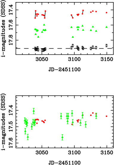
Figure 5: LQLM $i$-band light curves of FBQ 0951+2635. Top: A (filled circles), B $-$ 0.9 mag (filled triangles), and S3 $-$ 0.6 mag (open circles). Bottom: comparison between the A master record (filled circles) and the time- and magnitude-shifted light curve of B (filled triangles). See main text for details.

The top panel in Fig. 5 displays the LQLM light curves of the lensed quasar (A and B components) and the S3 star. Filled circles, filled triangles and open circles trace the behaviours of A, B (shifted by $-$0.9 mag) and S3 (shifted by $-$0.6 mag), respectively. There must be some diffuse contamination by the lens galaxy light, so the B fluxes in Table 3 and Fig. 5 are greater than the true ones. From the standard deviation of $m_{S3}$ over the whole monitoring period, we infer a typical error in the S3 fluxes of 17 mmag (see open circles and associated error bars). Hence, the typical uncertainty in the B fluxes should be larger than 17 mmag, since B is as bright as S3 ($\sim$ 18.5$-$18.6 mag), but it is located within a crowded region. Unfortunately, even using frames with $\langle{\rm FWHM}\rangle\sim$ 1$\aas@@fstack{\prime\prime}$2 and $\langle{\rm SNR}\rangle\sim$ 80, we cannot achieve 1$-$2% level photometry for B (some deviations between adjacent nights are relatively large).

Four pairs of adjacent fluxes of A show significant scatters around the mean values (in the top panel in Fig. 5, we draw four lines joining the members of each pair). For this reason, they are grouped (by computing four mean fluxes at the corresponding mean epochs) to obtain a master light curve, i.e., an accurate (smooth) trend that reliably describes the underlaying short-timescale variability. This master curve is depicted in the bottom panel of Fig. 5 (filled circles). Before the gap, the quasar has a small level of activity. However, after the gap, there is a 60-mmag gradient lasting about 30 days. Thus, the $R$-band and $i$-band records exhibit similar variability levels on a timescale of $\sim$ 2 weeks (see Fig. 3). To gain perspective on the nature of the observed variability in the $i$ band (A component), the B light curve is shifted in time (using the 16-day time delay by Jakobsson et al., 2005), and then is compared to the master light curve of A. We derive an average magnitude difference of 1.094 mag between the time-shifted record of B and the master curve of A (using bins with semi-size of 2–4 days). The time- and magnitude-shifted light curve of B is also included in the bottom panel of Fig. 5 (filled triangles). The typical error in the S3 fluxes is used as a lower limit for the uncertainty in the photometric measurements of B (see above). We find a clear agreement between the master curve of A and the adjacent fluxes of B, when these last fluxes are properly shifted in time and magnitude. Thus, there is no evidence of short-timescale extrinsic variability (due to microlensing or another phenomenon) in our $i$-band observations.

The new LQLM light curves of FBQ 0951+2635 allow us to measure an accurate flux ratio (corrected by the time delay) in the $i$ band: $A/B_{*}$ = 2.74 $\pm$ 0.02 (1$\sigma$). We do not measure the $i$-band flux ratio $A/B$ around day 3100 but the contaminated ratio $A/B_{*}$, where $B_{*}=B+G$ and $G$ is a contribution due to the lensing galaxy.

3.2 SDSS frame and recent evolution of $A/B$

The high-quality SDSS² $i$-band frame of FBQ 0951+2635 at day 2250 (FWHM = 0$\aas@@fstack{\prime\prime}$75 and SNR = 99) leads to a flux ratio $A/B_{*}$ = 2.8 $\pm$ 0.1 (1$\sigma$), in good agreement with the LQLM estimation. We note that $B_{*}=B+G$ (see above), and the uncertainty in the SDSS flux ratio incorporates both photometric and simultaneity errors. This last error is associated with the use of fluxes at the same time of observation, i.e., without time delay correction (see above). There is no evidence of an appreciable evolution in $A/B_{*}$ over days 2250$-$3100. This $i$-band result agrees with the Maidanak-SDSS recent trend of $A/B$ in the $R$ band (see filled circles and triangles from day 2250 to day 3100 in Fig. 4). Comparing the flux ratios in both optical filters, we may derive that the lens galaxy light in the $i$ band produces a plausible contamination of the B component in such filter ($\sim$ 130 mmag).

4 Conclusions

A previous analysis (Paraficz et al., 2006) showed the existence of extrinsic variability of the observer-frame optical continuum in the gravitationally lensed double quasar FBQ 0951+2635. The two quasar components (A and B) cross two different regions of the lensing galaxy, so distributions of collapsed objects could affect one (or both) of the light curves and then produce extrinsic variations. This microlensing hypothesis is more plausible for the B component because it crosses the central region of the galaxy (see Jakobsson et al., 2005). Paraficz et al. (2006) reported on two possible microlensing variabilities at red wavelengths in the 1999$-$2001 period: short-timescale events (B flares having a duration of months) or a gradient lasting a few years. Both alternatives can account for the 1999$-$2001 $R$-band observations, and this paper sheds light on the dominant kind of microlensing fluctuations occurring in FBQ 0951+2635.

We analyse new Maidanak $R$-band images taken in the 2001$-$2006 period (a 6-year homogeneous monitoring), and a few complementary frames in the $rR$ bands taken in 2004 and 2007 (SDSS and Maidanak/SI 600 Series archives). The Maidanak-SDSS flux ratios ($A/B$) in the red part of the optical continuum are inconsistent with the absence of long-timescale ($\sim$ years) gradients and the continuous production of B flares lasting a few months (short-timescale microlensing events). If this last scenario were true, all data points in Fig. 4 would be distributed between the two horizontal dashed lines. The whole set of flux ratios (from 1999 to 2007) favour the existence of a long-timescale microlensing fluctuation, so long-timescale gradients seem to be the dominant microlensing variations. While $A/B$ shows a bump in the 2003$-$2004 period, it is almost constant from late 2004 to the middle of 2007. This last quasi-stationary behaviour is supported by additional data in the $i$ band (from new LQLM images taken in 2007 and the SDSS archive frame in that filter). Gaynullina et al. (2005) and Paraficz et al. (2006) also found a long-timescale microlensing variation in the doubly imaged quasar SBS 1520+530. Although the existence of rapid flares in the early years of monitoring (1999$-$2001) cannot be ruled out, these hypothetical B flares are not produced in a continuous way. Short-timescale microlensing is not detected in the Maidanak variability study over the first semester of 2004. The LQLM data in the $i$ band also indicate the absence of short-timescale events in 2007. Apart from the 1999$-$2007 optical data, FBQ 0951+2635 has recently been observed in X-rays (Dai & Kochanek, 2009). However, the X-ray flux ratio has a large uncertainty and it is not useful for comparison with our estimates in the optical continuum.

If microlensing in the B component is the physical origin of the long-timescale fluctuation, this fluctuation represents a progressive demagnification of B followed by a quasi-stationary evolution in more recent epochs. The optical continuum flux ratio at red wavelengths is always below the Mg ii flux ratio (Jakobsson et al., 2005, see also Fig. 4), which is usually assumed to be weakly affected by microlensing. Thus, the recent microlensing magnification of B would be relatively weak, but still appreciable. The microlensing peak (maximum magnification of B) would have taken place before the discovery of the lens system by Schechter et al. (1998). Strictly speaking, the continuum flux ratio refers to the flux ratio in the $R$ band, i.e., a spectral region containing both the red continuum and the Mg ii emission line. However, this line only contributes a few percent to the broad band fluxes (see Fig. 4 of Schechter et al., 1998). It can be shown that the line-corrected ratio is very similar to the ratio from total fluxes in the $R$ band (see also Jakobsson et al., 2005). We also note that $A/B$ is not corrected by any extinction factor, so this flux ratio might be a biased estimator of the lens (macrolens + microlens) magnification ratio. For example, Falco et al. (1999) suggested the relative extinction of A by dust in the lensing galaxy. This dusty scenario leads to a true lens magnification ratio greater than $A/B$.

We point out that new flux ratios at a large collection of wavelengths should be key tools to discuss dust extinction and microlensing in the lensing galaxy (e.g., Wambganss & Paczynski, 1991; Falco et al., 1999; Goicoechea et al., 2005a, b; Elíasdóttir et al., 2006; Yonehara et al., 2008). Moreover, FBQ 0951+2635 must be imaged in the $rR$ bands during the next years (several times per year, with a 2-week separation between consecutive observations). This modest monitoring programme will lead to draw the future evolution of $A/B$, as well as to obtain relevant information on the structure of both the source quasar and the intervening galaxy (e.g., Wambsganss, 1990; Kochanek, 2004; Morgan et al., 2007).

References

- Adelman-McCarthy et al. (2008) Adelman-McCarthy J. K. et al., 2008, ApJS, 175, 297
- Artamonov et al. (1987) Artamonov B. P., Novikov S. B., Ovchinnikov A. A., 1987, in Gladyshev S.A., eds, Methods for increasing the efficiency of optical telescopes. Moscow State University, Moscow, p. 16
- Dai & Kochanek (2009) Dai X., Kochanek C. S., 2009, ApJ, 692, 677
- Ehgamberdiev et al. (2000) Ehgamberdiev S. A. et al., 2000, A&AS, 145, 293
- Eigenbrod et al. (2007) Eigenbrod A., Courbin F., Meylan G., 2007, A&A, 465, 51
- Elíasdóttir et al. (2006) Elíasdóttir Á., Hjorth J., Toft, S., Burud I., Paraficz D., 2006, ApJS, 166, 443
- Falco et al. (1999) Falco E. E. et al., 1999, ApJ, 523, 617
- Gaynullina et al. (2005) Gaynullina E. R. et al., 2005, A&A, 440, 53
- Goicoechea et al. (2005a) Goicoechea L. J., Gil-Merino R., Ullán A., 2005a, MNRAS, 360, L60
- Goicoechea et al. (2005b) Goicoechea L. J. et al., 2005b, ApJ, 619, 19
- Goicoechea et al. (2008) Goicoechea L. J. et al., 2008, NewA, 13, 182
- Jakobsson et al. (2005) Jakobsson P. et al., 2005, A&A, 431, 103
- Kochanek et al. (2000) Kochanek C. S. et al., 2000, ApJ, 543, 131
- Kochanek (2004) Kochanek C. S., 2004, ApJ, 605, 58
- Koptelova et al. (2005) Koptelova E. et al., 2005, MNRAS, 356, 323
- Morgan et al. (2007) Morgan C. W., Kochanek C. S., Morgan N. D., Falco E. E., 2007, ApJ, submitted, also available as arXiv:0707.0305
- Paraficz et al. (2006) Paraficz D., Hjorth J., Burud I., Jakobsson P., Elíasdóttir Á., 2006, A&A, 455, L1
- Schechter et al. (1998) Schechter P. L., Gregg M. D., Becker R. H., Helfand D. J., White R. L., 1998, AJ, 115, 1371
- Shalyapin et al. (2008) Shalyapin V. N., Goicoechea L. J., Koptelova E., Ullán A., Gil-Merino R., 2008, A&A, 492, 401
- Wambsganss (1990) Wambsganss J., 1990, PhD thesis (Munich University), also available as report MPA 550
- Wambganss & Paczynski (1991) Wambganss J., Paczynski B., 1991, AJ, 102, 864
- Williams et al. (2006) Williams K. A., Momcheva I., Keeton C. R., Zabludoff A. I., Lehár J., 2006, ApJ, 646, 85
- Yonehara et al. (2008) Yonehara A., Hirashita H., Richter P., 2008, A&A, 478, 95